Sage Journals: Discover world-class research

Abstract

The objective of this paper is to investigate the hydrodynamic characteristics of the transient flows around a 3D pitching hydrofoil via numerical studies, where the effects of tunnel wall boundary layer and gap flows are considered. Simulations are performed using an unsteady Reynolds Average Navier-Stokes solver and the k-ω SST turbulence model, coupled with a two-equation γ-Re_θ transition model. Hydrodynamic forces and flow structures are compared to the results with the equivalent 2D computations. During the upward pitching stage, the transition phenomenon is accurately captured by both the 2D and 3D simulations. The slightly lower lift and suction side loading coefficients predicted by the 3D simulation are due to the pressure effects caused by the tip gap flow. During the dynamic stall stage, the 2D case exhibits a clear overshoot on the hydrodynamic force coefficients and the 3D simulation results better agree with the experimental results. During the downward pitching stage, the flow transitions back to laminar. As for the effect of gap flow and the wall boundary condition, the gap flow causes disturbances to the formation and development of the vortex structures, resulting in the complex distribution of the three-dimensional streamlines and the particle path.

1. Introduction

In order to improve the aircraft maneuverability by using the dynamically induced lift which occurred in the dynamic stall phenomenon, as well as to avoid or reduce undesirable effects such as structural instabilities, flutter, and resonance, a substantial number of experimental [1 –3] and numerical [4 –8] investigations on aerodynamic stall have been conducted. Various dynamic stall flow control techniques have also been investigated to mitigate the large drag and pitching moment while maintaining the favorable lift increases simultaneously [9 –12]. In hydrodynamics-related fields, due to the spatially or temporally varying inflow and active/passive body motions, the effective angle of attack changes rapidly. It is of paramount importance to understand the hydrodynamic characteristics in transient flows around a pitching hydrofoil [13 –16]. In recent years, great progress has been made in the study of the transient flows around a pitching hydrofoil. Anderson et al. [17] conducted a series of tests to measure the force and power of harmonically oscillating foils in subcavitating flows. They showed that the moderately strong leading edge vortex interacts with the trailing edge vortex, resulting in the formation of a reverse Karman street. Ducoin et al. [18] conducted the combined experimental and numerical investigation of the transition from laminar to turbulence flow on a NACA66 hydrofoil undergoing a transient pitching motion at four pitching velocities. They found that increasing the pitching velocity tends to delay the laminar-to-turbulence transition and an increase of the hysteresis effect during pitch-down motion resulting in a significant increase of the hydrodynamic loading. However, the investigations in the past have been extensively on 2D hydrofoils, while the geometry together with 3D effect, turbulence, and unsteadiness makes the transient simulation still a challenging issue [19, 20]. It becomes necessary to simulate the 3D transient flows around a pitching hydrofoil to understand how the 3D flows and the pitching motions relate to each other.

The objective of this paper is to investigate the hydrodynamic characteristics of the transient flows around a 3D pitching hydrofoil via numerical studies, where the effects of tunnel wall boundary layer and gap flows between the free end of the hydrofoil and the test section wall are considered. The physical and numerical models are presented in Section 2. Detailed analysis of the transient flow around a pitching hydrofoil as well as the 3D effects on the dynamic behavior of transient flow structures is presented in Section 3. Finally, the conclusions, discussions, and future work are summarized in Sections 4 and 5.

2. Physical and Numerical Model

2.1. Conservation of Mass and Momentum

The incompressible and unsteady Reynolds Average Navier-Stokes (URANS) equations, in their conservative form, for a Newtonian fluid without body forces and heat transfers are presented below in the Cartesian coordinate:

\begin{matrix} \frac{\partial u_{j}}{\partial x_{j}} = 0, \\ \frac{\partial u_{i}}{\partial t} + \frac{\partial (u_{i} u_{j})}{\partial x_{j}} = - \frac{1}{ρ} \frac{\partial p}{\partial x_{i}} + \frac{1}{ρ} \frac{\partial}{\partial x_{j}} \times [(μ + μ_{t}) (\frac{\partial u_{i}}{\partial x_{j}} + \frac{\partial u_{j}}{\partial x_{i}} - \frac{2}{3} \frac{u_{i}}{x_{j}} δ_{i j})], \end{matrix}

(1)

where ρ is the fluid density, u is the velocity, p is the pressure, and μ and μ_t are, respectively, the laminar and turbulent viscosity. The subscripts i and j denote the directions of the Cartesian coordinates.

2.2. Turbulence Model

In the present simulation, the k-ω SST turbulence model [21] (corresponding to the Shear Stress Transport option in CFX with automatic wall function) is coupled with a two-equation γ-Re_θ transition model [22, 23], which is built on the local variables and compatible with modern CFD methods (corresponding to the Gamma Theta Model option in CFX [24])

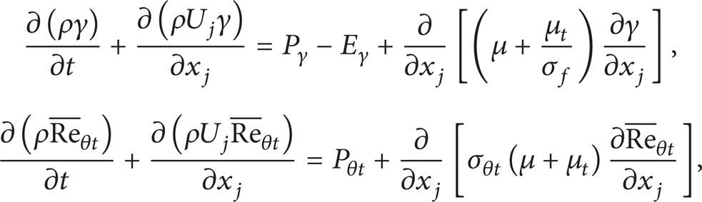
\begin{matrix} \frac{\partial (ρ γ)}{\partial t} + \frac{\partial (ρ U_{j} γ)}{\partial x_{j}} = P_{γ} - E_{γ} + \frac{\partial}{\partial x_{j}} [(μ + \frac{μ_{t}}{σ_{f}}) \frac{\partial γ}{\partial x_{j}}], \\ \frac{\partial (ρ {\bar{Re}}_{θ t})}{\partial t} + \frac{\partial (ρ U_{j} {\bar{Re}}_{θ t})}{\partial x_{j}} = P_{θ t} + \frac{\partial}{\partial x_{j}} [σ_{θ t} (μ + μ_{t}) \frac{\partial {\bar{Re}}_{θ t}}{\partial x_{j}}], \end{matrix}

(2)

where γ is intermittency, P_γ and P_θt are transition sources, E_γ is destruction/relaminarization, and ${\bar{Re}}_{θ t}$ is local transition Reynolds number. This model is able to capture the major transition effects and accurately predict the separation induced transition in the present case. It should be noted that the combined turbulence model and transition model have already been validated for the NACA 66 hydrofoil under the same flow conditions [25, 26].

2.3. Numerical Setup and Descriptions

Based on the commercial software ANSYS CFX and the finite volume method, both the 2D and 3D simulations are performed for the NACA66 hydrofoil in the present study. The computational domain and boundary conditions are presented in Figure 1, which is identical to the experimental setup [27], and the small gap (1 mm) between the free end of the hydrofoil and the test section wall is taken into consideration for the 3D case. A sliding interface is used at the boundary of a circular zone encapsulating the pitching hydrofoil and centered on its pitch center, which allows for a relative angular displacement between the external and near-body mesh zone and preserves the mesh quality in the foil vicinity at the same time. The results shown in this paper correspond to the pitching hydrofoil subjected to a nominal free stream velocity of U_∞ = 5 m/s, which yields a moderate Reynolds number of Re = U_∞c/ν = 7.5 × 10⁵, where c is the chord length and ν is the dynamic viscosity of the liquid.

Figure 1:

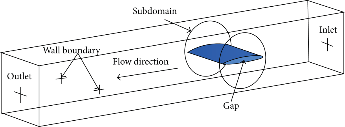
Computational domain and boundary conditions.

The 3D fluid mesh (shown in Figure 2) is composed of 1,850,000 structured elements and 10,000 unstructured elements with tetrahedron and hexahedron combined in the gap region. Mesh refinements are performed at leading and trailing edge of the foil and in the wake region and the structured boundary layer meshes were characterized by y⁺ = yu_τ/ν ≈ 1, where y is the thickness of the first cell from the foil surface and u_τ is the wall frictional velocity. The time step chosen for the simulation is Δt = 1 × 10^{− 4} s, which ensures that the averaged CFL = U_∞ × Δt/Δx ≈ 1.

Figure 2:

3D computational grids around the hydrofoil.

Considering the rotation center at x/c = 0.5 from the leading edge (LE), the variation of actual measured angle of attack is depicted in Figure 3, which is also used for the computations and is achieved by using the CFX user-defined code. The pitching motion is defined as a single upward-downward rotational motion of the foil from 0° to 15° and then back to 0° of the angle of attack, including the angular acceleration at the beginning and in the middle, as well as the angular deceleration in the middle and at the end of the pitching process. In this paper, numerical results are shown for the mean angular velocity of $\dot{α} = 2 α_{\max} / t_{f} = 6^{°} / s$ , where t_f is the total duration of the transient pitching motion, which is in accordance with the experiment [27]. For clarity, the upward phase of the pitching cycle is denoted by α⁺ and the downward phase by α⁻.

Figure 3:

Angle of incidence versus time.

3. Results

The 3D simulation of the instantaneous span-averaged lift ( $C_{L} = L / (0.5 ρ {U_{\infty}}^{2} s c)$ ), drag ( $C_{D} = D / (0.5 ρ {U_{\infty}}^{2} s c)$ ), and suction side loading (C_l⁺ (t) = ∑^{i = 1}₁₀ − C_P(x_i/c, t)Δ(x_i/c)) coefficients (where L and D are, respectively, the lift and drag, s is the span of foil, and C_p(x_i/c, t) is the pressure coefficient at x_i/c in the plane of midspan) with the geometric angle of attack α over one periodic cycle is compared to the associated 2D simulation, which has been also conducted by Ducoin et al. [18] and Huang et al. [28] for the same NACA66 hydrofoil, in Figure 4. The experimental results of the lift coefficients for the same foil at static are also shown in Figure 4(a) and that of the suction side loading [27] at dynamic can be referred to Huang et al. [26]. Comparing the 2D and 3D simulation results, the hydrodynamic force coefficients during one pitching process could be characterized by three stages: (I) during the upward pitching stage (from t₀ (α⁺ = 0°) to t₃ (α⁺ = 13.5°)), the lift coefficient C_l and the suction side loading coefficient C_l⁺ predicted by the 3D simulation are slightly lower than those for the 2D simulation results, while the drag coefficient C_d is higher. This is because C_l and C_l⁺ are affected by the pressure effects, while C_d is primarily affected by the 3D induced drag and hydrodynamic losses through the wall boundary layer and tip vortexes, which will be discussed in detail below. The predicted suction side loading coefficient C_l⁺ can obtain a good agreement with the experimental results and it should be noted that the experimental measured lift coefficients shown in Figure 4(a) are based on a static hydrofoil instead of a pitching one, to validate the transition phenomenon. (II) During the dynamic stall stage (from t₃ (α⁺ = 13.5°) to t₈ (α⁻ = 12°)), the 2D case exhibits a clear overshoot on the hydrodynamic force coefficients and three large amplitude fluctuations of the hydrodynamic coefficients are observed from the 2D simulation results, while the peak force for the 3D simulation results is much smaller and agrees better with the experimental results, especially for the third peak and trough. This is attributed to the influence of the shed vortexes dwelling over the suction side of the hydrofoil surface, which can be referred to the detailed discussion of the flow structures below. (III) During the downward pitching stage (from t₈ (α⁻ = 12°) to the end), the hydrodynamic force coefficients have similar trend to that during the upward pitching process, and the 3D effects, including the induced drag and the energy dissipation through the gap flow, as well as the wall boundary layer effects at the wall, have been ignored in the 2D case. Hence we mainly focus on the upward pitching stage and the dynamic stall stage in the present study.

Figure 4:

Evolution of the hydraulic characteristics with time.

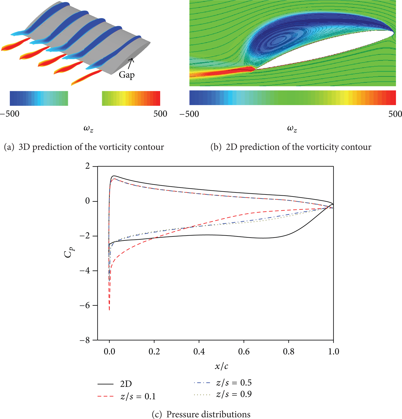
Figure 5 illustrates the coordinate system and slices distribution along the spanwise direction based on a top view. Figures 6 –11 show the predicted flow structures at representative times based on the simulational results of the 2D and 3D flow, respectively, in which the flow structures are visualized using contour slices of z-vorticity at five spans, as shown in Figure 5, and the 2D and 3D spanwise variation of the pressure distributions along the surface of the hydrofoil are also presented.

Figure 5:

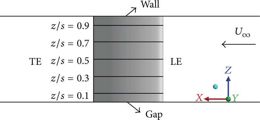
Illustration of slices along the spanwise direction.

Figure 6:

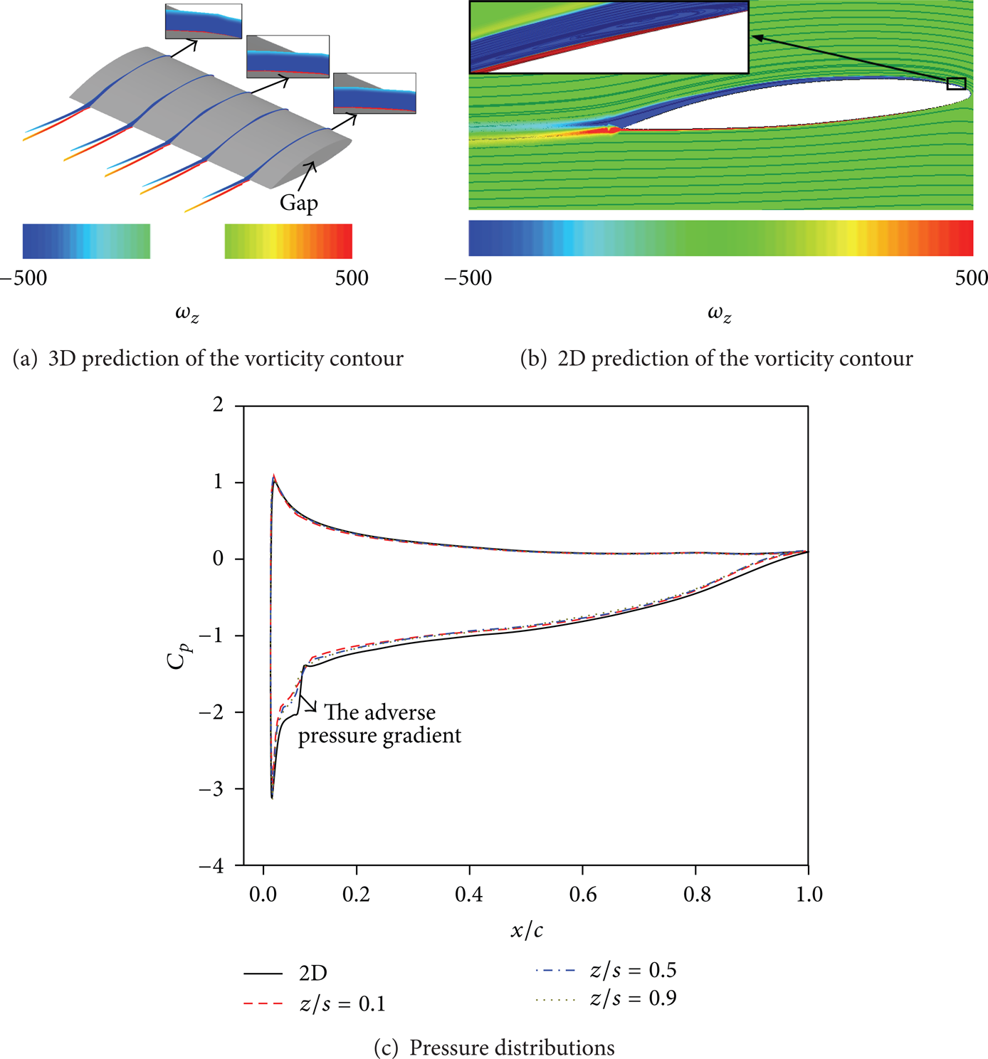
Comparison between 2D and 3D predictions at t₁ (α⁺ = 5.5°) during the pitching motion.

Figure 7:

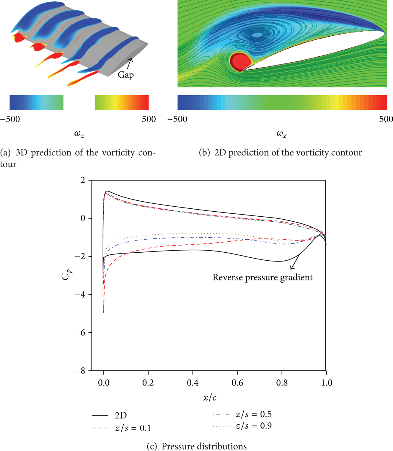
Comparison between 2D and 3D predictions at t₂ (α⁺ = 10°) during the pitching motion.

Figure 8:

Comparison between 2D and 3D predictions at t₃ (α⁺ = 13.5°) during the pitching motion.

Figure 9:

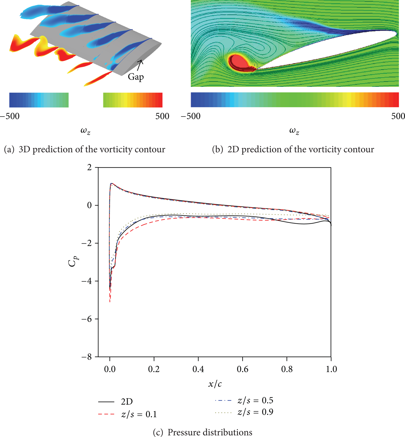
Comparison between 2D and 3D predictions at t₅ (α⁻ = 14.7°) during the pitching motion.

Figure 10:

Comparison between 2D and 3D predictions at t₆ (α⁻ = 14.4°) during the pitching motion.

Figure 11:

Comparison between 2D and 3D predictions at t₇ (α⁻ = 14.2°) during the pitching motion of the foil.

From t₀ (α⁺ = 0°) to t₃ (α⁺ = 13.5°), the lift and drag coefficients both increase with the angle of attack α, as shown in Figure 4. The inflection of the lift and suction side loading coefficient at t₁ (α⁺ = 5.5°) is caused by the laminar-to-turbulent transition near the leading edge of the foil, where the adverse pressure gradient is strong enough to separate the boundary layer and forces it to become fully turbulent. The transition phenomenon is accurately captured by both the 2D and 3D simulations, as shown in Figures 4 and 6(a)-6(b), with the adverse pressure gradient predicted by the 2D simulation being larger, as shown in Figure 6(c). Between t₂ (α⁺ = 10°) and t₃ (α⁺ = 13.5°), a counterclockwise (“−”) vortex develops near the trailing edge of the foil, as shown in Figures 6 and 7, which is responsible for the slope decrease of the lift and suction side loading coefficients. From Figure 6, the contour slices of z-vorticity change little with the span of the hydrofoil and the pressure profiles on the suction side of the foil for the 3D simulation are slightly higher than those for the 2D case, which is due to the influence of the tip gap flow, resulting in the smaller pressure differences between the pressure side and suction side of the foil. This is also responsible for the lower lift coefficient C_l and the suction side loading coefficient C_l⁺ predicted by the 3D simulation, as shown in Figure 4. As α increases, as shown in Figure 7, the trailing edge vortexes at each span of the foil develop on a different extent and the smaller region of the vortex is observed closer to the gap, corresponding to the higher pressures on suction side in the 3D simulation results. Comparing the 2D and 3D simulation results shown in Figure 4, the lift and suction side loading coefficients predicted by the 3D simulation are lower than those predicted by the 2D simulation, and the drag coefficients predicted by the 3D simulation are larger. This is mainly attributed to the disturbances of the complex vortical gap flow, driven by the pressure difference from the pressure side to the suction side of the foil, altering the pressure distribution and increasing the flow resistance along the surface of the hydrofoil.

From t₃ (α⁺ = 13.5°) to t₈ (α⁻ = 12°), the leading and trailing edge vortexes develop, interact with each other, and shed downstream. This is responsible for the three fluctuations of the hydrodynamic coefficients, as shown in Figure 4. Take one cycle from t₄ (α⁻ = 14.9°) to t₇ (α⁻ = 14.2°). Due to the formation and expansion of the leading edge vortex between t₄ (α⁻ = 14.9°) and t₅ (α⁻ = 14.7°), the lift and drag coefficients increase rapidly, as shown in Figure 4. At t₅ (α⁻ = 14.7°), the leading edge vortex expands to the maximum extent and fully attaches on the foil suction side, as shown in Figure 8, which is corresponding to the peak of the lift and suction side loading coefficient curve, as shown in Figure 4. The lift and suction side loading coefficients all undergo a sudden drop when the adverse pressure gradient, caused by the growth of the clockwise (“+”) trailing edge vortex, forces the leading edge vortex to shed downstream between t₅ (α⁻ = 14.7°) and t₇ (α⁻ = 14.2°), as shown in Figures 4 and 9. The local minimum of the lift and suction side loading coefficients at t₇ (α⁻ = 14.2°) is corresponding to the moment just before the total shedding of the vortexes, as shown in Figure 10. Compared to the 2D simulation results, the contour slices of z-vorticity with span reveal differences in the solution. The 2D simulation case shows strong and coherent vortices on the suction side of the foil, while, for the 3D simulation, the development of the leading and trailing edge vortex is suppressed when it is close to the gap, and the clockwise (“+”) trailing edge vortex, as well as the interaction between the leading and trailing edge vortex, can only be observed by the slices far away from the gap. Additionally, from Figures 8 –10, the pressure distribution at span of z/s = 0.1 is different from that at span of z/s = 0.5 and z/s = 0.9, and the minimum pressure amplitude near the leading edge of the foil suction side decreases due to the tip leakage vortex developing from the gap flow.

From t₈ (α⁻ = 12°) to the end, during the downward pitching process, the flow has similar trend to the upward pitching process and the flow transitions back to laminar.

To further explain the effects of gap and boundary layer on the 3D flow, Figure 12 relates the planar observation on various crossflow planes located at streamwise stations along the hydrofoil (see the planes A–D with x/c = 0.15, 0.50, 0.85, and 1.20, where x represents the distance to the head of the foil) to the previously described three-dimensional flow structures. On plane A, there is a near-wall flow along the − z direction, representing that the tip boundary condition significantly influences the flow field. From the streamline distribution shown in Figure 13 and the flow structures shown in Figure 14 by means of unsteady particle trace trajectories, it can be observed that, at the front part of the foil, large velocity gradient along the spanwise is responsible for a spanwise pressure gradient, resulting in the flow from the foil center plane toward the tip region. On planes B and C, which provide a cut through the vortex structures (seen in Figures 13 and 14), the velocity component with opposite direction is apparent, especially near the gap region, which is consistent with the spiraling streamlines distributed on the suction side of the foil, as shown in Figure 13. As shown in Figure 14, the liquid near the gap flows upward through the gap and causes disturbances to the formation and development of the vortex structures on the suction side, which can be seen in Figure 10(a). On plane D downstream of the vortex, there is a strong velocity component towards the foil center plane.

Figure 12:

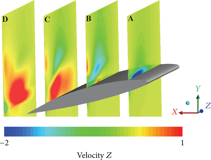
Contours of spanwise-velocity at t₆ (α⁻ = 14.4°).

Figure 13:

3D streamline distributions around the hydrofoil at t₆ (α⁻ = 14.4°).

Figure 14:

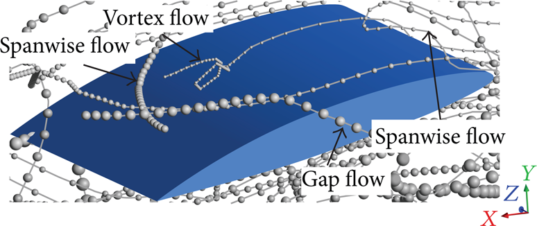
Particle trace trajectories in 3D flow from t₆ to t₆ + T.

A more detailed comparison of the velocity profiles at x/c = 0.15, 0.50, and 0.85 is provided in Figure 15. At x/c = 0.15, it flows much faster in the gap region (z/s = 0.01) near the surface with a much larger velocity gradient and then it reduces to the freestream velocity, while, at x/c = 0.50 and 0.85, the reverse flow near the surface can be clearly observed at span of z/s = 0.50 and 0.99, which cannot be found at span of z/s = 0.01 and the velocity gradient in the gap region decreases along the streamwise direction. It also accounts for the lower strength of the vortexes near the gap region and the partially attached vortex structures on the suction side of the hydrofoil, as shown in Figures 8 –10.

Figure 15:

Comparison of streamwise velocity profiles at x/c = 0.15, 0.50 and 0.85.

4. Conclusions

Numerical results are presented for a pitching NACA66 hydrofoil by the k-ω SST turbulence model coupled with a two-equation γ-Re_θ transition model. The effects of tunnel wall boundary layer and gap flows between the free end of the hydrofoil and the test section wall are investigated. The primary findings include the following.

Comparing the 2D and 3D simulation results, the hydrodynamic force coefficients during one pitching process could be characterized by three stages: the upward pitching stage, the dynamic stall stage, and the downward pitching stage. During the upward pitching stage, the lift coefficient C_l and the suction side loading coefficient C_l⁺ predicted by the 3D simulation are slightly lower than those for the 2D simulation results, while the drag coefficient C_d is higher, because the 3D effects, including the induced drag and the energy dissipation through the gap flow, as well as the wall boundary layer effects at the wall, have been ignored in the 2D case. During the dynamic stall stage, the 2D case exhibits a clear overshoot on the hydrodynamic force coefficients and three large amplitude fluctuations of the hydrodynamic coefficients are observed from the 2D simulation results, while the peak force for the 3D simulation results is much smaller and better agrees with the experimental results, especially for the third peak and trough, which is attributed to the influence of the shed vortexes dwelling over the suction side of the hydrofoil surface.

During the upward pitching stage, the transition phenomenon, which is responsible for the inflection of the lift and suction side loading coefficient when α⁺ = 5.5°, is accurately captured by both the 2D and 3D simulations. As the angle of attack increases, a counterclockwise (“−”) vortex develops near the trailing edge of the foil, which is responsible for the slope decrease of the lift and suction side loading coefficients. The contour slices of z-vorticity change little with the span of the hydrofoil and the pressure profiles on the suction side of the foil for the 3D simulation are slightly higher than those for the 2D case, which is due to the influence of the tip gap flow, while during the dynamic stall stage, the leading and trailing edge vortexes develop, interact with each other, and shed downstream. For the transient turbulent flow at high angle of attack, the leading and trailing edge vortexes exhibit significant 3D effects and the development of the vortex structures is suppressed when it is close to the gap, with the minimum pressure amplitude near the gap region decreasing due to the tip leakage vortex developing from the gap flow with steep pressure gradient and low minimum pressure.

As for the effect of gap flow and the wall boundary condition on the flow structures, the liquid near the gap will flow upward through the gap and cause disturbances to the formation and development of the vortex structures on the suction side. The flow in the gap region reduces the strength of the vortexes and the interaction between the leading and trailing edge vortex is weak near the gap, resulting in the vortex flow partially attached on the suction side near the gap instead of shedding downstream. Meanwhile, the spanwise perturbation can induce the creation of spanwise vorticity and the corresponding spanwise undulations; hence the distribution of the three-dimensional streamlines, as well as the particle path, is found to be quite complex.

5. Discussions and Future Work

Although reasonable agreements are obtained between the experimental and 3D numerical results, with the similar trend of the measured and predicted suction side lift coefficient observed, some discrepancies still exist in the dynamic stall region, which is probably attributed to the inadequacy of the conventional URANS to capture the flow details accurately especially when the flow is dominated by large-scale transient vortices. Higher fidelity simulations such as large eddy simulations (LES) would better illustrate the flow physics. For the pressure distribution along the surface of the hydrofoil, it is unfortunate that the load measurements are not available for the present case. To better validate and demonstrate the flow characteristics, additional experimental results would be added for the hydrofoil in the future work. As demonstrated in [29], the Eulerian approaches, such as streamlines, velocity vectors, and z-vorticity contours, are aiming at partitioning the flow based on the instantaneous distribution of a scalar field, while the particle-based Lagrangian approach, such as particle track, is concerned with patterns emerging from the advection of passive tracers. An approach based on the trajectory of point over a period of time, finite-time Lyapunov exponent (FTLE), has been proven to be useful to evaluate exact vortex boundaries in unsteady flow field, but more systematic validations are needed, particularly for the specific temporal and spatial resolution for the pitching foil cases. Further studies of the unsteady flow structures would be included in the future work. In addition, according to [18, 28], the pitching rate has significant effects on the transient flow, including the laminar-to-turbulence transition and the dynamic stall, as well as the three-dimensional flow characteristics. In the future, the influence of pitching rate on the flow response would be discussed further.

Conflict of Interests

The authors declare that there is no conflict of interests regarding the publication of this paper.

Footnotes

Acknowledgments

The authors would like to express our sincere gratitude to Professor Young (Department of Naval Architecture and Marine Engineering, University of Michigan, Ann Arbor, Michigan, USA) and Professor Antoine Ducoin (French Naval Academy Research Institute (IRENav), France; LHEEA Laboratory, Ecole Centrale de Nantes, Nantes, France) for their helpful comments and support to our work. Completion of this research would not have been possible without their support and understanding. The authors also gratefully acknowledge the support from the National Natural Science Foundation of China (Grant nos. 51306020 and 51239005) and the Natural Science Foundation of Beijing (Grant no. 3144034).

References

Raffel

Kompenhans

, and Wernert

, “Investigation of the unsteady flow velocity field above an airfoil pitching under deep dynamic stall conditions,” Experiments in Fluids, vol. 19, no. 2, pp. 103–111, 1995.

Lee

and Gerontakos

, “Investigation of flow over an oscillating airfoil,” Journal of Fluid Mechanics, vol. 512, pp. 313–341, 2004.

Mat

Ishak

I. S.

Lazim

T. M.

, “Development of delta wing aerodynamics research in Universiti Teknologi Malaysia low speed wind tunnel,” Advances in Mechanical Engineering, vol. 2014, Article ID 434892, 9 pages, 2014.

McCroskey

W. J.

, “Unsteady airfoils,” Annual Review of Fluid Mechanics, vol. 14, pp. 285–311, 1982.

Carr

L. W.

, “Progress in analysis and prediction of dynamic stall,” Journal of Aircraft, vol. 25, no. 1, pp. 6–17, 1988.

Carr

L. W.

and Chandrasekhara

M. S.

, “Compressibility effects on dynamic stall,” Progress in Aerospace Sciences, vol. 32, no. 6, pp. 523–573, 1996.

Ekaterinaris

J. A.

and Platzer

M. F.

, “Computational prediction of airfoil dynamic stall,” Progress in Aerospace Sciences, vol. 33, no. 11–12, pp. 759–846, 1998.

Sheng

Galbraith

R. A. M.

, and Coton

F. N.

, “Prediction of dynamic stall onset for oscillatory low-speed airfoils,” Journal of Fluids Engineering, vol. 130, no. 10, Article ID 101204, 8 pages, 2008.

Magill

J. C.

and McManus

K. R.

, “Control of dynamic stall using pulsed vortex generator jets,” in Proceedings of the 36th Aerospace Sciences Meeting and Exhibition, No. AIAA-1998–675, Reno, Nev, USA, 1998.

10.

Carr

L. W.

and McAlister

K. W.

, “The effect of a leading-edge slat on the dynamic stall of an oscillating airfoil,” AIAA Paper 1983–2533, 1983.

11.

Yen

and Ahmed

N. A.

, “Parametric study of dynamic stall flow field with synthetic jet actuation,” Journal of Fluids Engineering, Transactions of the ASME, vol. 134, no. 7, Article ID 071106, 2012.

12.

Karim

M. A.

and Acharya

, “Suppression of dynamic-stall vortices over pitching airfoils by leading-edge suction,” AIAA Journal, vol. 32, no. 8, pp. 1647–1655, 1994.

13.

Arndt

R. E. A.

, “Cavitation in fluid machinery and hydraulic structures,” Annual Review of Fluid Mechanics, vol. 13, pp. 273–328, 1981.

14.

Akcabay

D. T.

and Young

Y. L.

, “Hydroelastic response and energy harvesting potential of flexible piezoelectric beams in viscous flow,” Physics of Fluids, vol. 24, no. 5, Article ID 054106, 2012.

15.

Ducoin

and Young

Y. L.

, “Hydroelastic response and stability of a hydrofoil in viscous flow,” Journal of Fluids and Structures, vol. 38, pp. 40–57, 2013.

16.

Motley

M. R.

and Young

Y. L.

, “Performance-based design and analysis of flexible composite propulsors,” Journal of Fluids and Structures, vol. 27, no. 8, pp. 1310–1325, 2011.

17.

Anderson

J. M.

Streitlien

Barrett

D. S.

, and Triantafyllou

M. S.

, “Oscillating foils of high propulsive efficiency,” Journal of Fluid Mechanics, vol. 360, pp. 41–72, 1998.

18.

Ducoin

Astolfi

J. A.

Deniset

, and Sigrist

J.-F.

, “Computational and experimental investigation of flow over a transient pitching hydrofoil,” European Journal of Mechanics—B/Fluids, vol. 28, no. 6, pp. 728–743, 2009.

19.

Garmann

D. J.

and Visbal

M. R.

, “Numerical investigation of transitional flow over a rapidly pitching plate,” Physics of Fluids, vol. 23, Article ID 094106, 2011.

20.

Kinsey

and Dumas

, “Three-dimensional effects on an oscillating-foil hydrokinetic turbine,” Journal of Fluids Engineering, vol. 134, no. 7, Article ID 071105, 2012.

21.

Menter

F. R.

, “Improved two-equation k-ω turbulence models for aerodynamic flows,” NASA Technical Memorandu 34, 103975, 1992.

22.

Langtry

R. B.

and Menter

F. R.

, “Transition modeling for general cfd applications in aeronautics,” AIAA Paper 2005–522, Reno, Nevada, 2005.

23.

Menter

F. R.

Langtry

R. B.

, and Völker

, “Transition modeling for general purpose CFD codes,” Flow Turbulence Combustion, vol. 77, no. 1, pp. 277–303, 2006.

24.

ANSYS, ANSYS CFX 14.0 Help Document, ANSYS, 2011.

25.

Wang

G. Y.

, and Huang

, “Numerical methods and transition investigation of transient flows around a pitching hydrofoil,” IOP Conference Series: Materials Science and Engineering, vol. 52, no. 2, Article ID 022001, 2013.

26.

Huang

Ducoin

, and Young

Y. L.

, “Physical and numerical investigation of cavitating flows around a pitching hydrofoil,” Physics of Fluids, vol. 25, no. 10, Article ID 102109, 2013.

27.

Ducoin

, Etude experimentale et numerique du chargement hydrodynamique des corps portants en regime transitoire avec prise en compte du couplage fluide structure [Ph.D. thesis], Institut de Recherche de l'Ecole Navale, Brest Armées, France, 2008.

28.

Huang

, and Wang

, “Numerical simulation of unsteady cavitating flows around a transient pitching hydrofoil,” Science China Technological Sciences, vol. 57, no. 1, pp. 101–106, 2014.

29.

Wang

Huang

, and Bai

, “Lagrangian coherent structures analysis of gas-liquid flow in a bubble column,” Science China: Physics, Mechanics and Astronomy, vol. 57, no. 6, pp. 1169–1177, 2014.

Numerical Simulation of Transient Flows around a 3D Pitching Hydrofoil

Abstract

1. Introduction

2. Physical and Numerical Model

2.1. Conservation of Mass and Momentum

2.2. Turbulence Model

2.3. Numerical Setup and Descriptions

3. Results

4. Conclusions

5. Discussions and Future Work

Conflict of Interests

Footnotes

Acknowledgments

References