Benchmark Numerical Simulations of Viscoelastic Fluid Flows with an Efficient Integrated Lattice Boltzmann and Finite Volume Scheme

Abstract

An efficient IBLF-dts scheme is proposed to integrate the bounce-back LBM and FVM scheme to solve the Navier-Stokes equations and the constitutive equation, respectively, for the simulation of viscoelastic fluid flows. In order to improve the efficiency, the bounce-back boundary treatment for LBM is introduced in to improve the grid mapping of LBM and FVM, and the two processes are also decoupled in different time scales according to the relaxation time of polymer and the time scale of solvent Newtonian effect. Critical numerical simulations have been carried out to validate the integrated scheme in various benchmark flows at vanishingly low Reynolds number with open source CFD toolkits. The results show that the numerical solution with IBLF-dts scheme agrees well with the exact solution and the numerical solution with FVM PISO scheme and the efficiency and scalability could be remarkably improved under equivalent configurations.

1. Introduction

The nonlinear dependence between stress and the rate of strain presents considerable challenges for the modeling and simulation of the viscoelastic fluid flows. Mathematically, viscoelastic fluid flows could be modeled by a coupled partial differential equation (PDE) system involving the governing equations and the constitutive equation. The simulation of viscoelastic fluid flows is usually implemented by the so-called discrete elastic-viscous split stress (DEVSS) numerical strategy with the commonly used pressure correction algorithms such as SIMPLE [1] and PISO [2, 3]. The PDE system could be decoupled [4] and discretized into linear systems by such numerical schemes as finite volume method (FVM), finite difference method (FDM), and finite element method (FEM) and solved by iterative algorithms and then the continuity condition would be introduced in to correct the intermediate solutions until convergence. Although the iterative process involved in the above numerical scheme could guarantee second-order accuracy, it will reduce computational efficiency.

As a mesoscopic scheme, lattice Boltzmann method (LBM) is still mainly used for simulating the incompressible or weakly compressible Navier-Stokes equations [5, 6]. Due to its good locality and simplicity, LBM scheme could be parallelized (e.g., [7, 8]) and optimized (e.g., [9–12]) efficiently on various supercomputing platforms to carry out large-scale simulations that can never be done before, and some well-established parallel LBM frameworks, such as PowerFlow and OpenLB, are already available to simulate a wide range of complex flows in commercial and open-source community. LBM scheme has also attracted increasing attention for the simulation of viscoelastic fluid flows. Ispolatov and Grant [13] introduce a Maxwell-type external force decaying exponentially with time into LBM scheme to simulate the viscoelastic effects. Giraud et al. [14, 15] and Lallemand et al. [16] propose an LBM scheme for solving Jeffreys model in their works. Onishi et al. [17, 18] introduce an LBM scheme to simulate the evolution of polymer conformation, and the constitutive equations of Oldroyd-B and FENE-P model can be recovered from their model in simple shear flow. Malaspinas et al. [19, 20] and Su et al. [21] construct an LBM scheme to simulate the evolution of the viscoelastic stress components through discretizing the constitutive equation with a modified convection-diffusion lattice Boltzmann mechanism; however, the model fails to reasonably explain the unphysical diffusive term of the viscoelastic stress, and its discretization processes for different constitutive models are not general either.

To eliminate the disadvantages in the above numerical schemes, we proposed a novel ILFVE scheme for the simulation of viscoelastic fluid flows in our previous work [22], which inherits the efficiency and scalability of LBM and maintains the accuracy and generality of FVM. However, the spatial coupling scheme involves interpolation in every time step, and the time stepping scheme is formulated without considering the characteristics of different physical processes; therefore, the efficiency of ILFVE scheme will be undermined. In order to improve the efficiency, an efficient integrated bounce-back lattice Boltzmann and finite volume scheme with different time scales (IBLF-dts) is constructed upon ILFVE scheme for the simulation of viscoelastic fluid flows in this work. The spatial interpolation between LBM and FVM is eliminated with the help of the LBM bounce-back boundary treatment [23, 24], and the time scales for LBM and FVM are decoupled according to the relaxation time of flowing dynamics of solvent and viscoelastic effects of polymer [21], reducing redundant computation spatially and temporally. Critical numerical simulations have been carried out to validate IBLF-dts scheme in benchmark flows based on open source CFD toolkits of OpenFOAM and OpenLB. The results with IBLF-dts scheme have good agreement with the analytical solutions, the numerical solutions of FVM schemes, and the experiments results in publications, and the efficiency and scalability is significantly improved compared with that of FVM or ILFVE scheme under equivalent configurations.

The rest part of this paper is organized as follows. In Section 2, the mathematical model and ILFVE scheme are described briefly. In Section 3, the main idea of IBLF-dts scheme is explained in detail. In Section 4, comprehensive validations are carried out in benchmark flows to validate the effectiveness, spatial accuracy, and efficiency of IBLF-dts scheme. Finally, brief conclusions are presented in Section 5.

2. Mathematical Model and ILFVE Scheme

2.1. The Mathematical Model

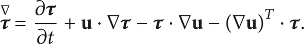
Mathematically, the isothermal and incompressible viscoelastic fluid flows could be modeled by a coupled partial differential equation system, including the governing equations and the constitutive equation. The motion of the polymer fluid is governed by the continuity equation

$\nabla ·\mathbf{u}=\mathrm{0}$

(1)

and the nondimensionalized Navier-Stokes equations

$\frac{\partial \mathbf{u}}{\partial t}+\mathbf{u}·\nabla \mathbf{u}=-\nabla p+\frac{\mathrm{1}}{\mathrm{Re}}\nabla ·\left(\mathrm{2}\beta \mathbf{D}+\mathit{\tau }\right)+\mathbf{g},$

(2)

where Re, u, p, and g represent the Reynolds number, the velocity, the pressure, and the body force of the polymer fluid. The viscosity ratio β = ν _s /(ν _s + ν _p ) is defined by the solvent viscosity ν _s and the polymer viscosity ν _p . The deviatoric stress is split into the viscous component of solvent 2βD and the polymeric contribution τ. D = 1/2(∇u + ∇u ^T ) is the strain rate tensor. τ is defined by different constitutive models, which could be constructed with phenomenological theory or molecular dynamics. Oldroyd-B model is a relatively simple but widely used constitutive model, given by

$\text{Wi}\stackrel{\nabla }{\mathit{\tau }}+\hspace{0.17em}\mathit{\tau }=\mathrm{2}\left(\mathrm{1}-\beta \right)\mathbf{D},$

(3)

where Wi is Weissenberg number, namely, the nondimensionalized relaxation time. $\stackrel{\nabla }{\mathit{\tau }}$ is the upper convected derivative of the viscoelastic stress tensor, mathematically defined as

$\stackrel{\nabla }{\mathit{\tau }}\hspace{0.17em}=\frac{\partial \mathit{\tau }}{\partial t}+\mathbf{u}·\nabla \mathit{\tau }-\mathit{\tau }·\nabla \mathbf{u}-{\left(\nabla \mathbf{u}\right)}^T·\mathit{\tau }.$

(4)

As can be seen, the solvent and polymer dynamics are only related to the viscosity ratio β and two dimensionless numbers Wi and Re, which are defined as

$\mathrm{Re}=\frac{u_{\mathrm{0}}{l}_{\mathrm{0}}}{{\nu }_s+{\nu }_p},\hspace{1em}\hspace{1em}\text{Wi}=\frac{\lambda u_{\mathrm{0}}}{l_{\mathrm{0}}},$

(5)

where the parameter with subscript 0 represents the characteristic quantity.

By introducing more degrees of freedom for the constitutive parameters in the constitutive equation, such as the elongational viscosity ɛ and the slip parameter ξ, the viscoelasticity of polymer fluid, especially some transient effects, could be characterized more faithfully in the form of partial differential equations. The detailed mathematical definition for other constitutive equation could be found in previous literature, such as Oldroyd-B model [25], PTT model [26, 27], and FENE model [28].

2.2. ILFVE Scheme

In previous works, we proposed an integrated ILFVE scheme to predict viscoelastic fluid flows. The incompressible Navier-Stokes equations are solved by classic lattice Boltzmann BGK scheme (LBGK model [29]), in which the external force term is calculated from the viscoelastic stress defined by arbitrary constitutive equations. The macroscopic parameters of density, velocity, and pressure of the fluid can be obtained from the evolution of particle distribution function f on specific lattice all together. The distribution function f at lattice node x could be expanded along each direction c _i as

$f_i\left(\mathbf{x}+{\mathbf{c}}_i,t+\mathrm{1}\right)-f_i\left(\mathbf{x},t\right)=-\frac{\mathrm{1}}{\tau }\left(f_i\left(\mathbf{x},t\right)-f_i^{\text{eq}}\left(\mathbf{x},t\right)\right)+{\mathbf{F}}_i,$

(6)

where x + c _i represents the next neighboring node along c _i , τ is the relaxation time of LBM model, and F _i is the discretized external force term which could be calculated by a second-order moment Guo-Zheng-Shi model [30]. f _i ^eq(x, t) is the Maxwell equilibrium distribution function determined by the model parameters and the macroscopic velocity. Given the initial states and the boundary conditions, the physical system could be simulated by the evolution of the distribution function with (6). The macroscopic parameters can be computed from f by

$\rho ={\displaystyle \sum }_{\mathrm{0}}^{m-\mathrm{1}}‍f_i,\hspace{1em}\hspace{1em}\mathbf{u}=\frac{\mathrm{1}}{\rho }{\displaystyle \sum }_{\mathrm{0}}^{m-\mathrm{1}}‍f_i+\frac{\mathrm{1}}{\mathrm{2}}\mathbf{F}.$

(7)

Pressure is defined by the ideal gas law p = c _s ²ρ.

The constitutive equation is integrated in the framework of FVM, using the velocity field obtained from the LBGK model. Most spatial derivative terms could be converted into a linear combination of the values of neighboring cells. By integrating the constitutive equation over each control volume at each time step, a linear algebraic system could be formulated about τ as follows:

$A\mathit{\tau }=\mathbf{S},$

(8)

where the coefficients matrix A contains the contributions from the convection and the diffusion fluxes as defined by the constitutive equation and S is the source term unrelated to the coefficients. Because A is a sparse diagonally dominant matrix, it could be solved with some iterative techniques, such as the conjugated gradient algorithm (CG) to obtain τ.

The two processes of LBM and FVM are integrated with the smallest time scale with a dimensional and spatial coupling scheme. Firstly, the calculation of LBM and FVM must be performed in uniform dimensional systems. Because the simulation of the incompressible Navier-Stokes equations depends only on Reynolds number [31], the equivalent LBGK model should be constructed with the characteristic values and Reynolds number in the real physical system. The dimensional transformation equation could be constructed through dimensional analysis. The transformation equation for the massless force ${\mathcal{C}}_{\text{LBM},P}\hspace{0.17em}(\nabla ·{\mathit{\tau }}^P)$ from FVM to LBM is defined as

${\mathbf{F}}^{\text{LBM}}=\frac{{\left(u_{\mathrm{0}}^{\text{LBM}}\right)}^{\mathrm{2}}\Delta x}{{\left(u_{\mathrm{0}}^P\right)}^{\mathrm{2}}}\nabla ·{\mathit{\tau }}^P,$

(9)

and the transformation equation for the velocity ${\mathcal{C}}_{P,\text{LBM}}\left(\mathbf{u}\right)$ from LBM to FVM is defined as

${\mathbf{u}}^P=\frac{u_{\mathrm{0}}^P}{u_{\mathrm{0}}^{\text{LBM}}}{\mathbf{u}}^{\text{LBM}},$

(10)

where the superscripts P and LBM of the parameters indicate the dimensional system of FVM and LBM. The parameter with a subscript 0 is the characteristic value, F is the massless force of LBM model, and Δx is the cell size of mesh. Secondly, the calculation of LBM and FVM must be performed on equivalent spatial positions. As in Figure 1, the computational domain is discretized with uniform cartesian grids; however, when applying the regularized boundary condition [32] for LBM scheme, there would exist a spatial offset between two grids, and the physical parameters such as the velocity and the viscoelastic stress must be interpolated from on grid to another at every time step. The spatial interpolation could reduce the efficiency and the numerical stability of the integrated scheme.

Figure 1:

The grid mapping between FVM and LBM in ILFVE scheme. The solid dots and crosses represent the centers of grid control volumes of FVM and grid nodes of LBM, respectively. The distance vector arrow r points from source interpolation node to target interpolation node.

3. IBLF-dts Scheme

IBLF-dts scheme is formulated upon ILFVE scheme to integrate bounce-back LBGK model and FVM in the same framework to simulate the isothermal incompressible Navier-Stokes equations and the constitutive equation, respectively, in which a specific coupling scheme is constructed to ensure a seamless data transformation between the two schemes. In order to improve the efficiency, the bounce-back boundary treatment for LBM is introduced in to improve the grid mapping of LBM and FVM, and the two processes are also decoupled in different time scales according to the relaxation time of polymer and the time scale of solvent Newtonian effect.

3.1. Grid Mapping

As the calculations of LBM and FVM are implemented on structured cartesian grids, their grid mapping must be considered firstly when integrating these two schemes in a specific hybrid simulation, which is determined by the boundary treatment of LBM scheme. According to the geometric mapping of the grid boundary with the fluid boundary, the boundary treatment of LBM scheme could be categorized as the wet boundary condition and the bounce-back boundary condition. For wet boundary condition, the grid boundary coincides with the fluid boundary, and the macroscopic parameters of the fluid can be recovered from the distribution function of the boundary nodes through Chapman-Enskog expansion just as the internal nodes. The wet boundary condition, such as the regularized boundary condition [32], Inamuro boundary condition [33], and Zou/He boundary condition [34], is applicable to various boundary constraints and gives second-order accuracy; therefore, it is applied in ILFVE scheme as in Figure 1. However, if wet boundary LBM grid is coupled with the FVM grid, there could be a half-cell-size offset between their grid nodes; thus, shared parameters should be interpolated from one grid to another.

The bounce-back boundary treatment for LBM is integrated into IBLF-dts scheme to improve the grid mapping of LBM and FVM. For bounce-back boundary condition, the fluid boundary locates somewhere half-way between a boundary node and the next fluid node as in Figure 2, enabling LBM grid nodes to coincide with the center of the control volumes on regular cartesian grid. The outmost boundary nodes are implemented to reflect the outgoing distribution functions of the boundary nodes back into the fluid again. The full-way bounce-back scheme and half-way bounce-back scheme [23] are similar in boundary geometric mapping but give different spatial accuracy [35, 36]. The half-way bounce-back scheme is second-order accurate to handle the no sip boundary condition theoretically and can also be manipulated to implement a Dirichlet condition with arbitrary velocity [24] or pressure [37]; therefore, it is implemented in simulation here. The grid mapping for IBLF-dts scheme could eliminate the spatial interpolation and thus improve the numerical stability and the computational efficiency.

Figure 2:

The grid mapping between FVM and LBM in IBLF-dts scheme. The solid dots and crosses represent the centers of grid control volume of FVM and grid nodes of LBM, respectively, L is the cell size. The bounce-back boundary condition is applied on the fluid boundary for LBM.

3.2. Time Scales Mapping

The two processes of LBM and FVM in IBLF-dts scheme are decoupled in different time scales by overall consideration of the characteristics of different dynamics and numerical schemes. Firstly, there are usually different time scales for different dynamics. The complex physics of viscoelastic fluid flows, originating from the interaction of polymer and solvent, can be decomposed into two separated but coupled dynamics of the polymer viscoelasticity and the macroscopic Newtonian effect. For viscoelastic fluid flows, the Newtonian effect usually evolves at a smaller time scale than the polymer viscoelasticity; therefore, the NS equations may reach equilibrium state in a much shorter time than the constitutive equation [21, 38]. To simulate all dynamics at smallest time scale could introduce computational redundancies, and we could increase the time step size for the dynamics with slow time evolution to improve efficiency. On the other hand, the time step size for different numerical schemes to reach convergence varies a lot. Theoretically, LBM and FVM are explicit and implicit second-order numerical schemes, respectively. Usually the implicit numerical scheme can employ larger time step size than the explicit one; therefore, FVM can introduce relatively larger time step size for the same dynamics.

The time stepping scheme for IBLF-dts is illustrated in Figure 3. N _t time steps of the NS equations are coupled with one time step of the constitutive equation in a basic temporal integration cycle in IBLF-dts scheme. At the beginning of each cycle, the macroscopic physical variables, such as u, p, and τ, will be transformed into each processes. The time step size for the coupled nonlinear PDEs system involves too many factors including the characteristics of physical processes and the stability, the convergence, and accuracy requirements; therefore, it is no way to formulate an accurate definition about the time step size in such systems; however, some semiquantitative analysis about the time step ratio could still be made under the careful consideration of the physical and numerical restrictions. The restriction for the time step size of LBGK model can be derived from error analysis [31]. As LBGK model gives second-order spatial accuracy, the lattice error would scales like ɛ(δx) ~ (δx)² = (Δx/l₀ ^P )²; meanwhile, as the spatial resolution is improved, the compressibility effects error would increase with higher Mach number, which scale like the square Mach-number ɛ(Ma) ~ Ma². The compressibility error could be rewritten as ɛ(Ma) ~ (u₀^LBM/c _s )² = (u₀ ^P Δt _s /Δxc _s )² through dimensional analysis. By overall consideration of these two factors, a sensible thing is to keep these two error terms at the same order as ɛ(δx) ~ ɛ(Ma) to maintain the overall accuracy. Therefore, restriction for the time step size Δt _s for LBGK model could be obtained as

$\Delta t_s~\frac{\mathrm{1}}{\mathrm{Re}}{\left(\Delta x\right)}^{\mathrm{2}}.$

(11)

Figure 3:

Time scales mapping for IBLF-dts scheme. Δt _s is the time step size for the Navier-Stokes equations and N _t is the ratio of time step size of the constitutive equation to that of the Navier-Stokes equations.

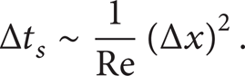
As can be seen in the constitutive equation (3), the time integration of viscoelastic stress is closely related to two model parameters Wi and β. The transient initial response of viscoelastic stress is more rapid at smaller Wi; therefore, smaller time step size is necessary under this kind of configuration. On the other hand, the polymer viscosity (1 − β)ν would also impact the steady viscoelastic stress, and higher polymer viscosity would give high steady stress value. Therefore, smaller time size would be required to maintain relative small time variation of stress under larger polymer viscosity. Therefore, a semiquantitative relationship of the time step size for the constitutive equation with the dimensionless number Wi and β could be given by

$\Delta t_p~\frac{\text{Wi}}{\mathrm{1}-\beta }.$

(12)

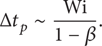
If only the physical parameters related to LBGK model and the constitutive model are considered (the spatial resolution is fixed here), we could define the time step ratio N _t from (11) and (12) as

$N_t=\frac{\Delta t_p}{\Delta t_s}~\frac{\text{Wi}\hspace{0.17em}\mathrm{Re}}{\mathrm{1}-\beta }.$

(13)

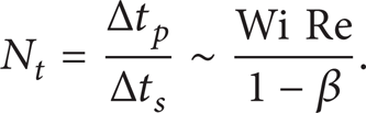
When carrying out the simulation of viscoelastic fluid flows with the hybrid scheme, Δt _s is defined first a according to (11), and then we could try out proper Δt _p under the guidance of (13). As the implicit integration for the constitutive equation is relatively expensive, the asynchronous time stepping scheme will significantly improve the computational efficiency while maintaining the accuracy of simulation.

3.3. The Parallel Numerical Algorithm for IBLF-dts Scheme

The detailed numerical algorithm for IBLF-dts scheme is listed as follows, where Ω[pid] is the subdomain distributed to processor pid, the superscripts P and LBM of the parameters indicate the dimensional system of FVM and LBM, the dimensional transformation function ${\mathcal{C}}_{Dx,Dy}\hspace{0.17em}\left(X\right)$ converts the dimension of a parameter from system D _x to system D _y as defined in (9) and (10).

The numerical algorithm is parallelized with a multiblocks structure in order to carry out large-scale simulation on parallel platforms, in which the discretized computational domain is decomposed into load-balanced rectangle subdomains Ω[pid] and distributed into different processors for simultaneous calculation (Algorithm 1). The boundary data of Ω[pid] must be refreshed before local operation in Steps 5 and 11, and the global residual must be aggregated and synchronized across all processors in Step 5 too; these data exchanges are implemented through underlayer parallel communication interface such as MPI and MPICH. In order to make analysis of the whole domain, all separated solutions for different subdomains would be reconstructed together as a whole in Step 17.

Algorithm 1:

Parallel IBLF-dts scheme based on multiblocks structure.

4. Numerical Validation

A coupling framework for IBLF-dts scheme is constructed upon open source CFD toolkits. The open source lattice Boltzmann codes OpenLB are integrated into the finite volume framework OpenFOAM as an independent LBM solver, and a coupling module is formulated to ensure the seamless data transfer between the FVM solver and the LBM solver. Critical numerical simulations have been implemented upon the coupling framework to validate the effectiveness, the spatial accuracy, and the efficiency of IBLF-dts scheme in different benchmark flows such as two-dimensional Poiseuille flow, Taylor-Green vortex, and lid-driven Cavity flow.

In the following part, N is defined as the spatial resolution for the characteristic length. N _t is the time scales ratio. Without loss of generality, Re ≤ 1 is taken in all the following simulations in order to validate the viscoelastic effects of the viscoelastic fluid flows under vanishingly low Reynolds number.

4.1. Poiseuille Flow

Firstly, the effectiveness and spatial accuracy of IBLF-dts scheme are validated in planar Poiseuille flow by comparing the numerical solution of IBLF-dts scheme with the analytical solution of Oldroyd-B viscoelastic fluid. As sketched in Figure 4, the geometry of the planar Poiseuille flow is defined as a planar tube of W × H. The inlet and the outlet of the tube are defined as cyclic boundaries, and the half-back back boundary conditions are applied on the fixed walls. The fluid in the tube flows from the inlet to the outlet driven by a constant body force g _x (or pressure difference) in direction x.

Figure 4:

The schematic diagram for the geometry of planar Poiseuille flow. g _x represents the body force driving the flow, u₀ is the max steady velocity component in x direction at the centerline of the tube.

The formulas of exact transient solutions for 2D Poiseuille Oldroyd-B viscoelastic flow are defined in [39]. Exact transient solutions are solved as formulas in MATLAB for comparison. After relative long time, a steady velocity profile that is exactly similar to that of Newtonian flow may be obtained at y direction. If related parameters are nondimensionalized as

$y^{*}=\frac{y}{H},\hspace{1em}\hspace{1em}{t}^{*}=\frac{{\nu }_{\mathrm{0}}}{H^{\mathrm{2}}}t,\hspace{1em}\hspace{1em}{u}_x^{*}=\frac{\mathrm{1}}{u_{\mathrm{0}}}{u}_x,\hspace{1em}\hspace{1em}{\tau }^{*}=\frac{H}{\eta u_{\mathrm{0}}}\tau ,$

(14)

where the characteristic velocity u₀ = g _x H²/8ν₀ is the max steady velocity at the centerline of the tube, then the steady velocity and viscoelastic stress components profiles along axis y could be given by

$\begin{array}{c}{u}_x^{*}(y^{*},t^{*})=\mathrm{4}{y}^{*}(\mathrm{1}-y^{*}),\\ {\tau }_{xx}=\mathrm{2}\text{Wi}(\mathrm{1}-\beta ){\left(\frac{\partial u^{*}}{\partial y^{*}}\right)}^{\mathrm{2}},\\ {\tau }_{xy}=(\mathrm{1}-\beta )\left(\frac{\partial u^{*}}{\partial y^{*}}\right),\\ {\tau }_{yy}=\mathrm{0},\end{array}$

(15)

where the variable with superscript “*” is the dimensionless parameter.

The simulations are run at β = 0.1, Re = 1, and N = 100W = H. The time step size for the NS equations is fixed as Δt = 1 × 10^{− 6} as Re is the same in all simulations and N _t = 50/100 is preset for λ = 0.5/1. At the beginning of simulation, all polymers are relaxed to their equilibrium state in the static fluid. Numerical solutions of the transient velocity at the centerline of the tube are plotted in Figure 5 for Wi = 0.5/1, and Figure 6 demonstrates the profiles of the viscoelastic stress components τ _xx and τ _xy on fixed walls of the tube for Wi = 0.5/1. As can be seen in Figures 5 and 6, because of the elastic memory effect of the polymer chains, there would be a transient fluctuation in the velocity and the viscoelastic stress of the fluid when it is accelerated by the body force at the beginning.

Figure 5:

The comparison of the analytical and numerical transient velocity at the centerline of the tube for Re = 1, Wi = 0.5/1, and N _t = 50/100.

Figure 6:

The comparison of the analytical and numerical transient stress component τ _xx and τ _xy on fixed walls of the tube for Re = 1, Wi = 0.5/1, and N _t = 50/100.

After a relatively long time, the polymer chain in the fluid will stretches to its equilibrium state under the interaction of the viscous and viscoelastic effects, and the fluid would reach a steady state finally. The steady velocity and viscoelastic stress profiles at x = H/2 with respect to y for Wi = 0.5/1 are plotted in Figures 7 and 8, respectively. As can be seen in Figures 5 and 6, the numerical results agree well with the analytical solutions of Oldroyd-B fluid for different Wi under reasonable N _t .

Figure 7:

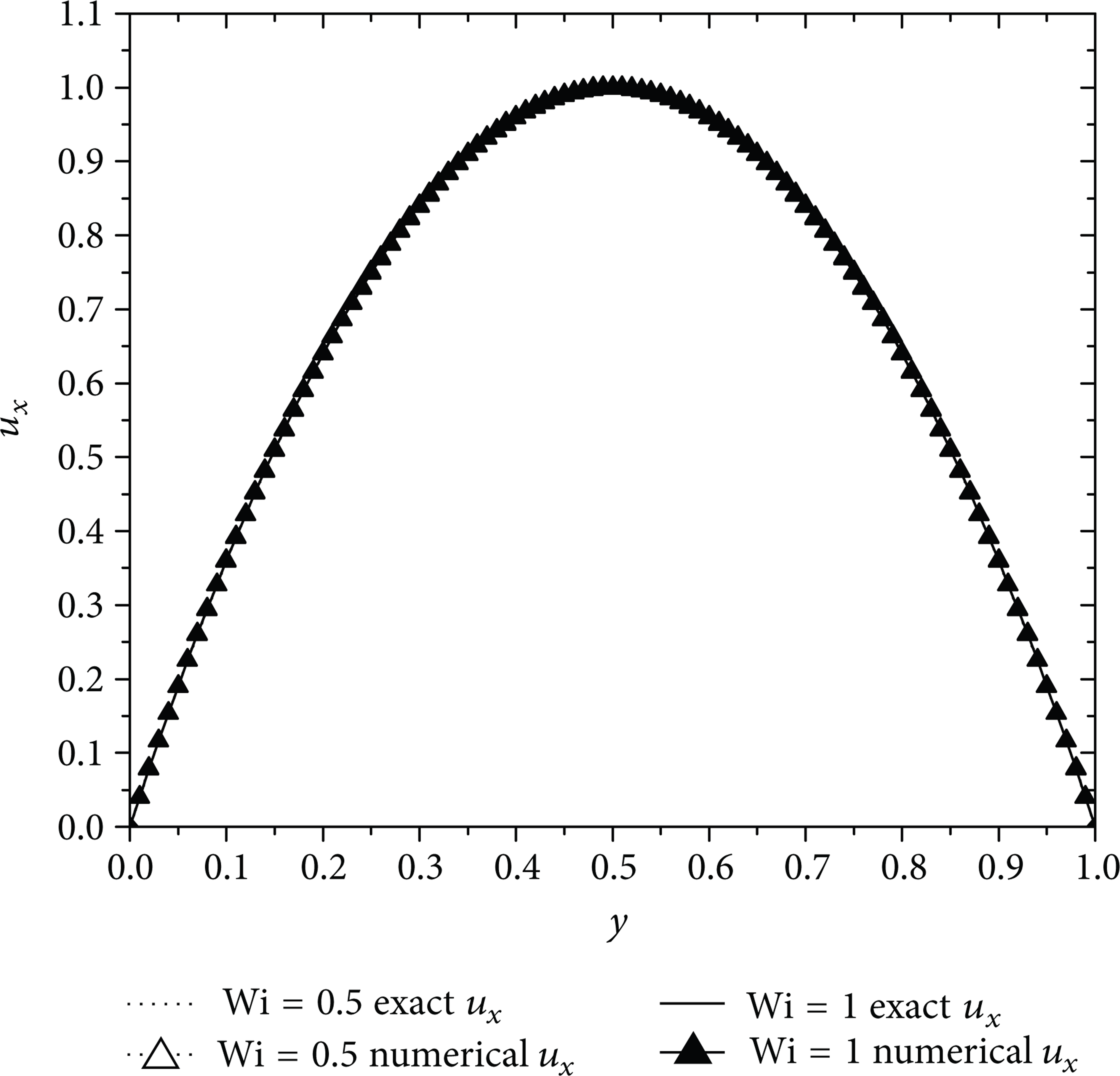
The comparison of the analytical and numerical steady velocity with respect to y for Wi = 0.5/1, N _t = 50/100.

Figure 8:

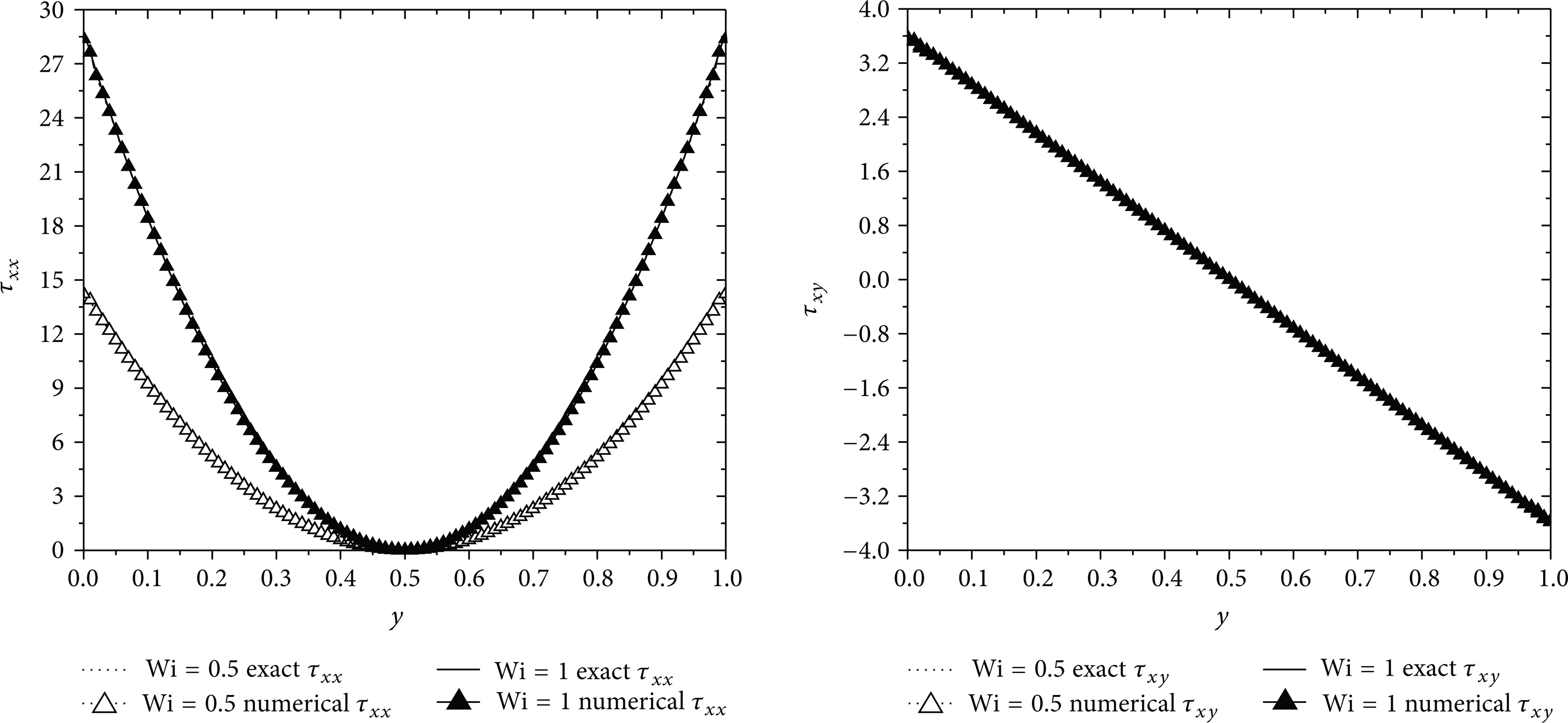
The comparison of the analytical and numerical steady stress components τ _xx and τ _xx with respect to y for Wi = 0.5/1, N _t = 50/100.

The numerical spatial accuracy would be discussed in what follows. Since the half-way bounce-back LBM scheme and FVM scheme give second-order accuracy theoretically, the IBLF-dts scheme would be second-order accurate also. The errors of the steady numerical solutions with IBLF-dts scheme are calculated with the analytical solutions defined in (15). Figure 9 displays the average error profiles for the steady velocity and the viscoelastic stress components in whole computational domain for N = 25/50/100/200. As can be seen in Figure 9, the error profiles are parallel to the line of slope = − 2, showing that the errors are decreasing with order two accordingly as the grid resolution increases.

Figure 9:

The numerical error of IBLF-dts scheme for Wi = 0.1 and N = 25/50/100/200.

4.2. Taylor-Green Vortex

In order to validate IBLF-dts scheme, the numerical solutions of planar Taylor-Green vortex with IBLF-dts scheme will be compared with those obtained with FVM PISO scheme [4] in this section. The geometry of planar Taylor-Green vortex is defined as a enclosed cavity of H × H. The cyclic boundary condition is applied on all walls. The pressure and velocity field of the fluid are initialized as follows [40]:

$\begin{array}{c}{u}_x(x,y)=u_{\mathrm{0}}\sin \left(\frac{\mathrm{2}\pi x}{H}\right)\cos \left(\frac{\mathrm{2}\pi y}{H}\right),\\ u_y\left(x,y\right)=-u_{\mathrm{0}}\cos \left(\frac{\mathrm{2}\pi x}{H}\right)\sin \left(\frac{\mathrm{2}\pi y}{H}\right),\\ p\left(x,y\right)=\frac{\mathrm{3}}{\mathrm{16}}\rho u_{\mathrm{0}}^{\mathrm{2}}\left(\cos \left(\frac{\mathrm{4}\pi x}{H}\right)+\cos \left(\frac{\mathrm{4}\pi y}{H}\right)\right),\end{array}$

(16)

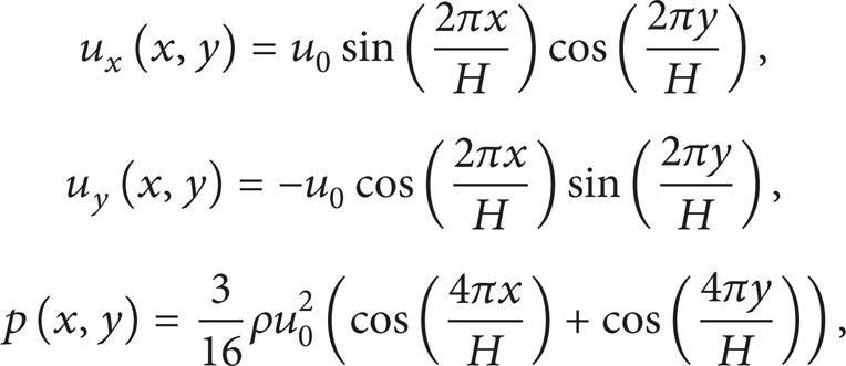
and the viscoelastic stress is set to zero across the whole domain at t = 0. The average kinetic and polymer energies could be defined as

$\begin{array}{c}{E}_{\text{kinetic}}=\frac{\mathrm{1}}{M}{\displaystyle \sum }_i‍\frac{\mathrm{1}}{\mathrm{2}}{\left|{\mathbf{u}}_i\right|}^{\mathrm{2}},\\ {\overline{E}}_{\text{polymer}}=\frac{\mathrm{1}}{M}{\displaystyle \sum }_i‍\frac{\mathrm{1}}{\mathrm{2}}\mathrm{tr}\left(\left|{\mathit{\tau }}_i\right|\right),\end{array}$

(17)

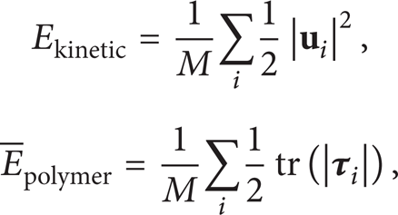
where M is the total cells number in the whole domain and i is the grid node index. Four symmetric vortices would appear at (0.25H, 0.25H), (0.25H, 0.75H), (0.75H, 0.25H), and (0.75H, 0.75H) after the initialization, and then the kinetic energy and polymer energy would keep evolving and changing into each other with the deformation of the fluid.

The constitutive model of the fluid is set as linear PTT model with the viscosity ratio β = 0.1, the slip parameter ξ = 1, and the elongational viscosity ɛ = 0.25. The Re of the incompressible Navier-Stokes equations is taken to 1, which is simulated by LBM D2Q9 model. The spatial resolution and time scales ratio are fixed as N = 100 and Δt = 1 × 10^{− 6}. N _t = 50/100 is preset for λ = 0.5/1. The kinetic energy profiles with IBLF-dts scheme are sketched in Figure 10 for different Wi. For Wi = 0, the constitutive model reduces to a Newtonian flow without any elastic memory effect; therefore, the kinetic energy would decrease smoothly with the time because of the internal friction of the fluid. However, for Wi > 0, the fluid would demonstrate obvious viscoelastic effects with the kinetic energy profiles winding around the profile of Wi = 0 until all energy dissipates over.

Figure 10:

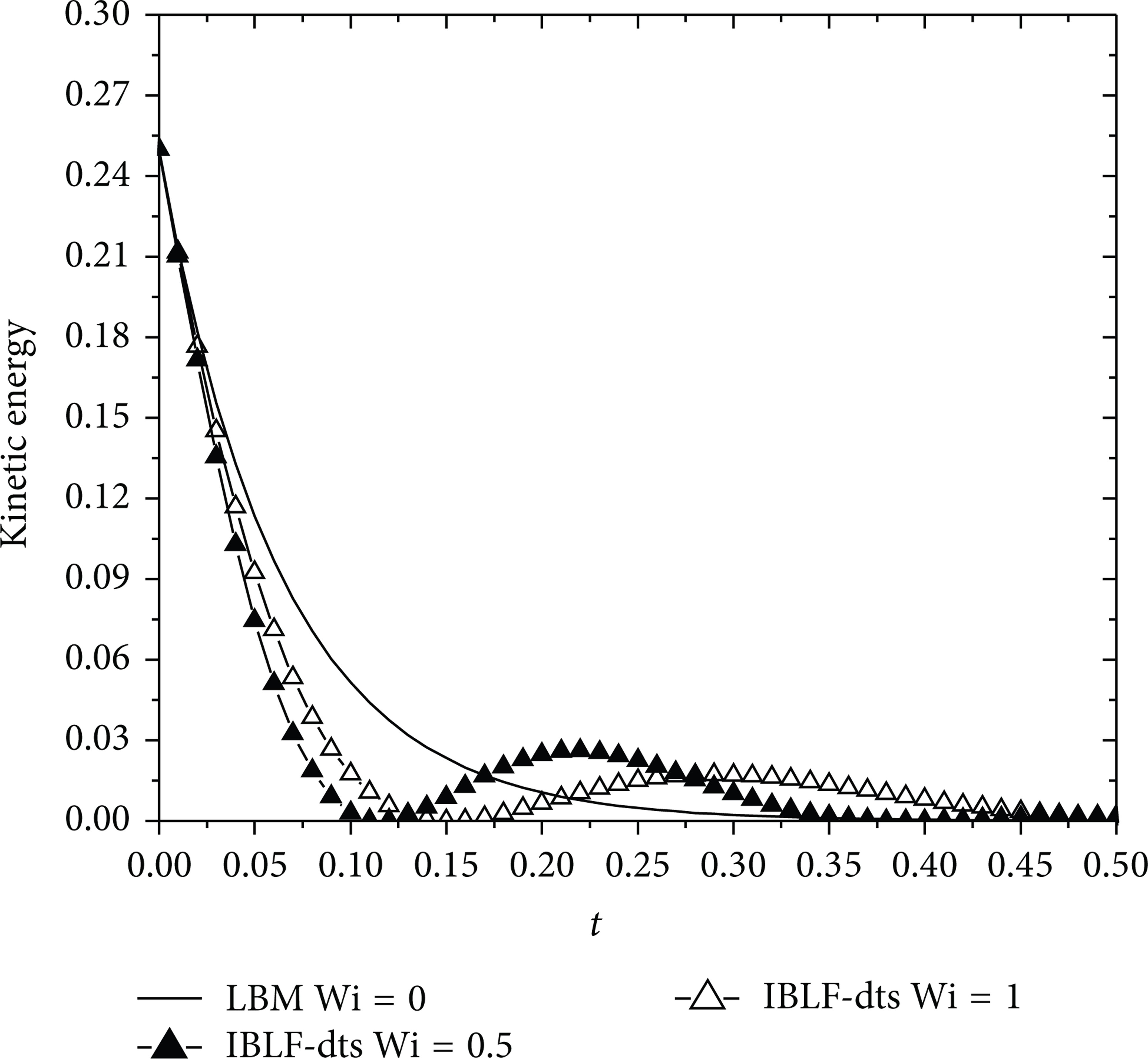
The comparison of the kinetic energy of Taylor-Green vortex for Wi = 0/0.5/1. The viscosity for incompressible solvent is the same in all simulations.

The numerical solutions of the energy with IBLF-dts scheme and FVM PISO scheme are also plotted in Figure 11 for comparison. The energy fluctuations observed in numerical simulations could be explained as follows. At the beginning of the simulation, the polymer molecules are at their equilibrium state everywhere. Then, the polymer chains begin to stretch under the deformation of the fluid, and the vortices intensity would decrease accordingly as part of the kinetic energy of the fluid is transformed into the polymer energy. When the inertial force is not strong enough to resist the elastic force, the polymer chains would give back part of their energy into the fluid, and the vortex will reverse and accelerate again. As can be observed in Figures 10 and 11, the numerical predictions of viscoelastic effects in Taylor-Green vortex with IBLF-dts scheme are in good agreement with those of FVM PISO scheme.

Figure 11:

The comparison of kinetic energy and polymer energy of Taylor-Green vortex obtained with FVM PISO scheme and IBLF-dts scheme for Re = 1, Wi = 0.5/1, and N _t = 50/100.

4.3. Lid-Driven Cavity Flow

In this section, the IBLF-dts scheme will be validated in lid-driven cavity flow by comparing the numerical solutions with some semiquantitative experiments results in previous publications [41, 42]. The lid-driven cavity flow refers to the recirculatory motion of a fluid confined in a enclosed rectangle cavity of H × H, which is usually driven by a constant velocity u of the upper rigid boundary. The steady motion of the fluid includes a core-vortex flow in the central region of the cavity and two secondary corner-vortex flows in the lower corner regions, and the vortices structure is sensitive to the viscoelastic effects of the polymer fluid.

We take β = 0.5, Re = 0.5, N = 100, and Δt = 1 × 10^{− 6} as in previous work [43] for all simulations here. N _t = 10/100 is preset for λ = 0.1/1. The half-way bounce-back boundary conditions are applied on cavity walls for LBM model, with a moment correction on the moving wall, and the zero-gradient boundary condition is applied for viscoelastic stress in the framework of FVM. The affection of viscoelastic effects to the vortex structure is observed in simulations for Wi = 0.1/1. The singularity of the flow field at the upper corners would cause numerical schemes to diverge; therefore, we chose the regularized boundary condition for velocity u [43] given by

$u\left(x,t\right)=\mathrm{8}\left(\mathrm{1}+\tanh \mathrm{8}\left(t-t_{\mathrm{0}}\right)\right){\left(\frac{x}{H}\right)}^{\mathrm{2}}{\left(\mathrm{1}-\frac{x}{H}\right)}^{\mathrm{2}},\left(\mathrm{0}\le x\le H\right),$

(18)

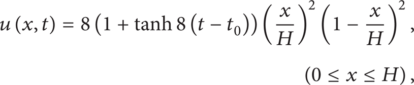
where t₀ is a preset threshold to smooth the time derivative and x is the distance of the current node from the upper left corner. The discontinuity of the velocity field at the two upper corners has been removed in (18).

The vortex intensity grows as the upper lid accelerates and reaches a steady state finally under low Reynolds number as the polymer energy builds up. The structure of the core vortex is sensitive to the Re and Wi of the fluid. The steady streamlines in the cavity are plotted in Figure 13 for Wi = 0.1/1, respectively. Because of the viscoelastic effects of the polymer chains, the flow in the cavity loses its fore-aft symmetry about the centerline x = H/2, and the main vortex shifts downstream with increasing Wi. The magnitude of this shift increases significantly with increasing Wi. As a consequence of the fluid incompressibility, the asymmetry of the vortex causes the radius of curvature of the local streamline near the upstream corner to increase while that in the corresponding downstream corner varies in the opposite way. The predicted viscoelastic effects agree well with those in the experiments in publication [41].

The contours of the steady viscoelastic stress tensor components for Wi = 0.1/1 are illustrated, respectively, in Figure 12. τ _xx has a thin but very sharp boundary layer along the moving lid. All three components have largest gradients near the upper corners, especially in the vicinity of the downstream corner, because the polymer chains are highly compressed or elongated in the upper right corner. It can also been observed that these localized maxima are located slightly away from the actual corner where the magnitude of the stress is expected to increase considerably and demonstrate a singular behavior. The stress conformation here is also in good agreement with the published experiment results [41].

Figure 12:

The contour of viscoelastic stress components τ _xx , τ _xy , and τ _yy of lid-driven cavity flow for Wi = 0.1/1, N _t = 10/100 obtained with IBLF-dts scheme.

Figure 13:

The streamlines of lid-driven cavity flow for Wi = 0.1/1 obtained with IBLF-dts scheme.

4.4. Efficiency and Scalability

With the benchmarks above, the efficiency and scalability of parallel IBLF-dts scheme are also compared to those of FVM PISO scheme and ILFVE scheme. The time complexity of numerical schemes involves a variety of factors such as the initial state, the numerical algorithm, the grid size, and the time step size. For simplicity and fairness, the solvers are not specially optimized for specific computer architecture or parallel framework. The initial configurations, such as the the time step size, the total simulation time, and the spatial resolution, are kept the same in all simulations.

In Figure 14, the simulation time of ILFVE scheme in different benchmark flows is decomposed into different parts for analysis, including solving τ, coupling τ, solving u, and coupling u. The spatial interpolation and the dimensional transformation are merged into one coupling step for convenience. As can be seen, solving τ is very expensive in ILFVE scheme and occupies the most part of the total time, whereas solving u with LBM is much more efficient than solving τ. The time for coupling τ, solving u, and coupling u is approximately the same and shows a linear relation with the spatial resolution; however, solving τ has a higher-order time complexity than the other parts. Therefore, it will contribute to the efficiency of simulation by extending the time step of solving τ and eliminating the spatial interpolation.

Figure 14:

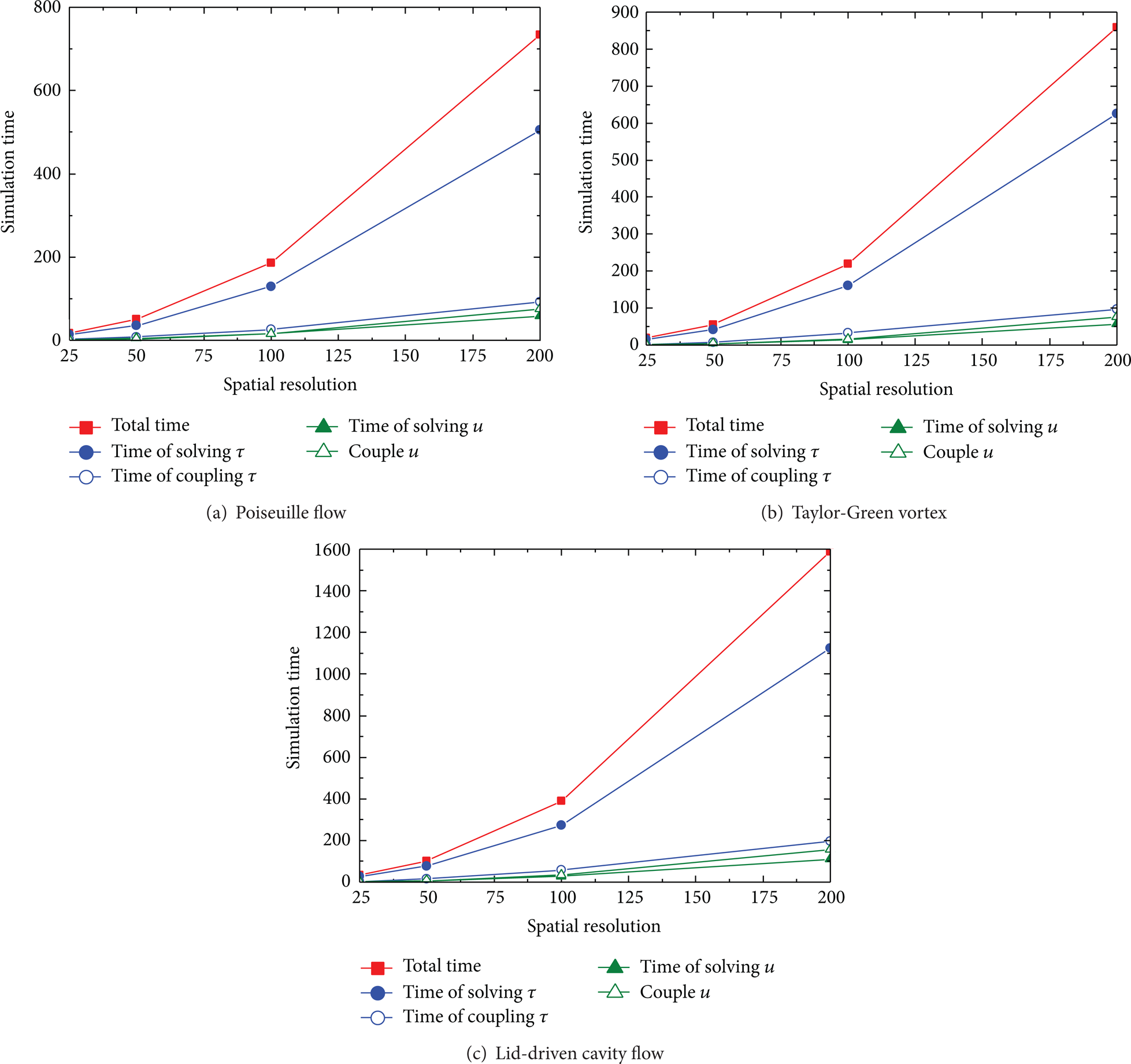
The simulation time of different parts of IBLF-dts scheme in different benchmark flows with different spatial resolutions.

In Figure 15, the efficiency of IBLF-dts scheme (N _t = 1) is compared with that of ILFVE scheme in different benchmark flows under equivalent configurations. Because the boundary layer of LBGK model has little influence on the total efficiency, the efficiency of IBLF-dts scheme (N _t = 1) makes no difference with that of ILFVE scheme except including an extra spatial interpolation operation in a single time step; therefore, the performance improvement obtained from new grid mapping scheme could be validated through comparing the simulation time of IBLF-dts (N _t = 1) to that of ILFVE scheme. As can be seen, the normalized time varies in different benchmarks, because the convergence of the algorithm would be greatly influenced by the configurations of the flow. By eliminating the spatial interpolation, the efficiency of IBLF-dts increases by approximately 10% to 25% compared with that of ILFVE scheme in simulations here. This proportion decreases with respect to the mesh resolution, as the time of solving τ would dominate other parts in high spatial resolution.

Figure 15:

The simulation time for different benchmark flows with IBLF-dts scheme. The time is normalized by that with ILFVE scheme under equivalent configurations.

The efficiency of IBLF-dts scheme with different N _t is also compared to that of FVM PISO algorithm in different benchmark flows under the same initial configurations in Figure 16, where the simulation time is normalized with that of FVM PISO algorithm. The results show that IBLF-dts scheme can yield much better efficiency than FVM PISO scheme, for it eliminates the pressure correction loop for solving the NS equations and extends the time step of solving τ. As can be seen, the simulation time of IBLF-dts is only 20% of that of PISO algorithm under same configurations where N _t is set to 1. Under certain accuracy requirement, increasing N _t will not change the compute load for solving the Navier-Stokes equations, but will reduce the time for solving the constitutive equation proportionally; therefore, the computational efficiency would be greatly improved. As can be seen, the simulation time of parallel IBLF-dts scheme with N _t = 10/50/100 is almost 17.5%/9.9%/8.6% of that with N _t = 1 for 2D Poiseuille flow and 16.1%/8.5%/7.4% for Taylor-Green vortex. However, the total simulation time does not decrease in proportion to N _t , because the time for solving τ will increase when extending the time step size to a certain extent.

Figure 16:

The efficiency of IBLF-dts scheme with N _t = 1/10/50/100 in different benchmark flows. The time is normalized by that with FVM PISO scheme under equivalent configurations.

The scalability of parallel IBLF-dts scheme and FVM PISO scheme is also evaluated on TianHe-2 supercomputer with the open source parallel toolkits. The speedups of both numerical schemes with 5 × 10⁶ cells are listed in Figure 17. For relative low parallelism (N_proc < 128), linear speedup would be observed, as all processors are confined in the same node or cabinet with higher communication speed. As N_proc increases, processors may be distributed across the whole system, and nonlinear speedup would appear because of the influence of IO operations and communications. When these unfavorable factors take over, the scalability of parallel scheme would reach its inflection point. In simulations here, FVM achieves its max speedup at N_proc ≈ 1024, whereas IBLF-dts reaches its max speedup at N_proc ≈ 1280. As can be seen, IBLF-dts could improve the scalability to a certain extent, because there is less global communication in its implementation compared to FVM PISO scheme.

Figure 17:

The comparison of scalability of FVM PISO scheme and IBLF-dts scheme on TianHe-2 for 5 × 10⁶ cells.

5. Conclusion

In this work, an efficient IBLF-dts scheme is proposed to integrate the bounce-back LBM and FVM schemes to solve the Navier-Stokes equations and the constitutive equation, respectively, for the simulation of viscoelastic fluid flows. Some brief conclusions can be made as follows.

1. IBLF-dts scheme is an efficient hybrid numerical scheme to simulate viscoelastic fluid flows. It can inherit the efficiency and scalability of LBM and maintain the accuracy and generality of FVM.

2. IBLF-dts scheme gives second-order spatial accuracy as FVM PISO scheme and LBM scheme.

3. The new grid mapping scheme and the decoupled time scales for IBLF-dts scheme could remarkably improve the efficiency of the simulation of viscoelastic fluid flows.

4. The scalability of parallel IBLF-dts scheme implemented with open source toolkits can also be improved to a certain extent.

Conflict of Interests

The authors declare that there is no conflict of interests regarding the publication of this paper.