Sage Journals: Discover world-class research

Abstract

This paper presented a novel procedure based on the ensemble empirical mode decomposition and extreme learning machine. Firstly, EEMD was utilized to decompose the vibration signals into a number of IMFs adaptively and the permutation entropy of each IMF was calculated to generate the fault feature matrix. Secondly, a new extreme learning machine was proposed by combining ensemble extreme learning machine and the evolutionary extreme learning machine which used an artificial bee colony algorithm to optimize the input weights and hidden bias. The proposed diagnosis algorithm was applied on the three rolling bearing fault diagnosis experiments. The numerical experimental results demonstrated that the proposed method had an improved generalization performance than traditional extreme and other variants.

1. Introduction

Rolling element bearings, as crucial components, are frequently used in a wide variety of rotating machinery, and their failure is one of the most reasons which lead to fatal breakdowns of machines [1]. Unexpected bearing failures could interrupt industrial production and cause unscheduled downtime and economic losses. Therefore, it is very important to be able to diagnosis the type and severity of the faults accurately and automatically for preventing the rolling element bearing from failures. It is proven that the performance of a fault diagnosis system is highly dependent on the amount of information contained within the extracted fault features and the classification ability of the classifier [2]. Hence, how to extract the fault characteristic information from the measurement signals and identify the fault type are considered as the crux of rolling element and draw a lot of attention for the researchers [3 –5].

Vibration signal analysis has been widely used as the most common and reliable method to extract fault features. Because of the factors such as nonlinear stiffness and clearances of rolling elements, the vibration signals of the rolling element bearings present nonstationary and nonlinear characteristics and common signal processing techniques which aim towards linear vibration signals, including time-domain and frequency-domain analysis, and consequently cannot handle the vibration signal of the rolling element bearings. Therefore, it is expected that the signal processing method should have good resolution in both time and frequency domains. The wavelet transform (WT) was the famous time-frequency signal analysis method and applied in many field [4]. However, WT needs to select appropriate base function and the decomposition scales cannot be changed. Empirical mode decomposition (EMD) was proposed as a self-adaptive decomposition scheme to overcome the deficiencies of WT. EMD is based on the local characteristic time scales of a signal and could decompose the complicated signal into complete and almost orthogonal components named intrinsic mode functions (IMFs) which represent the natural oscillatory mode embedded in the signal [6]. EMD shows outstanding performance in processing nonlinear and nonstationary signals than WT and has been applied in the field of fault diagnosis of rotating machinery [7]. Nevertheless, the mode mixing problem, which is defined as either a single IMF consisting of components of widely disparate scales, or a component of a similar scale residing in different IMFs is one of the most shortcoming of the EMD. Ensemble empirical mode decomposition (EEMD) is proposed to eliminate the mode mixing problem of EMD by adding finite white noise to the investigated signal [8]. Many researchers have proven that EEMD method outperforms the EMD and has lately attracted significant attention in fault diagnosis [9, 10]. Once a fault occurs in the bearing, the corresponding resonance frequency components are produced. Consequently, the distribution situation of the energy and frequency resonance in the different IMFs would change [11]. Many researchers focused on the fault features extraction based on IMFs decomposed by EEMD to find more accurate characteristic information. Lei et al. [12] used EEMD and Hilbert transform effectively to diagnose the rub-impact fault of a power generator and a heavy oil catalytic cracking machine set. Zhang and Zhou [13] extracted two types of features referred to as energy entropy and singular values based on EEMD. Guo et al. [14] utilized EEMD with spectral kurtosis to recover the impulses generated by bearing faults from the raw signal successfully. In recent years, nonlinear parameter identification techniques, such as approximate entropy (ApEn) [15] and sample entropy (SampEn) [16], have been investigated and selected as a tool for the rolling bearing fault diagnosis, and they show a better performance than the traditional feature extraction methods. Permutation entropy (PE) was a recently introduced increasingly valuable tool to characterize nonlinear time series [17]. PE has a merit of using only the order of the values and can detect dynamic change in complex systems more effectively compared with other tradition method [18]. However, the vibration signal has multiple spatiotemporal scales and original PE with single-scale based measures may lead to misleading results [19]. Therefore, this paper proposed a novel feature extraction method named Intrinsic Mode Permutation Entropy (IMPE), which utilized PE to extract the fault information at the different scale.

Fault classification is another important task in fault diagnosis. After feature extraction, an intelligent classifier is needed to indicate the fault type accurately and automatically. Although many approaches were developed to build fault classifier, including Bayesian network, neural networks, rough set theory, and support vector machines (SVM), all these methods have some drawbacks such as the poor generalization ability on the small samples and the model parameter selection and training speed [20]. Extreme learning machine (ELM) was a novel powerful machine learning method based on single hidden layer feed forward networks and has been proven to have better generalization performance and fast learning speed compared to traditional algorithms [21]. Nevertheless, the ELM algorithm randomly chooses input weights and hidden bias and employs the Moore-Penrose (MP) generalized pseudoinverse to calculate the output weights, and the randomly assigned parameter will introduce an unoptimal performance of classifier [22]. In literature [23, 24], the authors used evolutionary algorithm, such as differential evolution (DE) and the article bee colony (ABC), to determine global optimal input weights and hidden nodes biases. The evolutionary ELM has relative better classification performance ability than the original ELM. Moreover, evolutionary ELM needs less node numbers than the original which increases the effectiveness. On the other hands, the ensemble version of ELM named EE-ELM was proposed to improve the classification accuracy [25]. EE-ELM has been proven to show the better robust classification performance than ELM, but it shows lower classification accuracy than evolutionary ELM. So as to guarantee stable and accurate classification result, we combined the advantage of two types ELM and proposed a novel variant of ELM named ensemble optimal ELM (EO-ELM) for multifault classification in this paper.

The rest of the paper is organized as follows. Section 2 presents the IMPE method in this study. Section 3 introduces the multiclass EO-ELM classifier and the proposed diagnosis method. Section 4 details experiment results and a discussion is given to demonstrate the effectiveness of the proposed algorithm. Finally, a brief conclusion is offered in Section 5.

2. Intrinsic Mode Permutation Entropy

2.1. A Brief View of EEMD

EEMD was proposed as an effective noise-assisted method to alleviate the drawback of the mode mixing problem of EMD. The EEMD algorithm was given as follows [8].

Step 1. Give the number of ensembles K and the amplitude of the added white noise initially. Set the trial number k = 1.

Step 2. Add an artificially white noise with the given amplitude to the investigated signal x(t) to generate a new signal as follows:

x_{k} (t) = x (t) + n_{k} (t),

(1)

where n_k(t) denotes the kth added white noise series and x_i(t) represents the noise-added signal of the kth trial, while k = 1, 2, …,K.

Step 3. The noise-added signal x_k(t) is decomposed into IMFs by using the original EMD algorithm as follows:

x_{k} (t) = \sum_{m = 1}^{M} c_{m, k} (t) + r_{m, k} (t),

(2)

where M denotes the number of IMFs, r_m,k(t) denotes the residue components in decomposing result of EEMD, and c_m,k(t) represents the mth IMF of the kth trial which includes different frequency components.

Step 4. If k < K, then go to Step 2 with k = k + 1. Different white noise series is added at each time to obtain an ensemble of IMFs.

Step 5. Calculate the ensemble means of the corresponding IMFs of the decomposition as the final result:

{\bar{c}}_{m} (t) = \frac{1}{K} \sum_{k = 1}^{K} c_{m, k} (t),

(3)

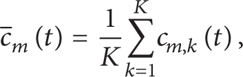
where ${\bar{c}}_{m} (t)$ is the final IMFs results decomposed by EEMD, while m = 1, 2, …,M, and k = 1, 2, …,K.

2.2. Permutation Entropy and IMPE

Given a time series {x(t),t = 1, 2, …,N}, this time series could be embedded in m-dimensional phase and the reconstructed vectors X(t) can be calculated as follows [18]:

X (t) = {x (t), x (t + τ), \dots, x (t + (m - 1) τ)},

(4)

where m is the embedded dimension and τ is the time delay. Then the m sample points of data contained in each X(t) can be sorted in an increasing order as follows:

{x (t + (j_{1} - 1) τ)} \leq {x (t + (j_{2} - 1) τ)} \leq \dots \leq {x (t + (j_{m} - 1) τ)} .

(5)

If x(t + (j₁ − 1)τ) = x(t + (j₂ − 1)τ), their original positions can be sorted according to the index j_*. That is, when j₁ ≤ j₂, x(t + (j₁ − 1)τ) ≤ x(t + (j₂ − 1)τ) can be written.

Consequently, any vector X(t) can be mapped onto a group of symbols as

S (l) = (j_{1}, j_{2}, \dots, j_{m}),

(6)

where S(l) is one of the m! different symbol permutations, which is mapped onto the m number symbols (j₁,j₂,…,j_m). P₁,P₂,…,P_k denote the probability distribution of each symbol sequence, respectively, and the permutation entropy of order m for the time series {x(t),t = 1, 2, …,N} can be defined as the Shannon entropy for the k symbol sequences as

H_{p} (m) = - \frac{1}{\ln (m!)} \sum_{j = 1}^{J} p_{j} \ln (p_{j}),

(7)

where the factor 1/ln⁡(m!) is a normalization factor such that 0 ≤ H_p/ln⁡(m!) ≤ 1. The PE measures the randomness of the time series. The smaller the value is, the more regular the time series is; otherwise, the series is more random.

To sum up, the proposed IMPE consists of two main steps. Firstly, EEMD decomposes the vibration signal and acquires the IMFs of EEMD. Secondly, the PE of each IMF should be computed to construct the fault characteristic vector. Compared with the PE, IMPE can characterize signal regularity at the different levels and could extract the nonlinear fault feature information. Therefore, we utilized the IMPE as the feature extraction method in this paper and the detailed performance result of IMPE is discussed in Section 4.

3. Ensemble Optimal Extreme Learning Machine

3.1. Brief Introduction of Extreme Learning Machine

Given the N arbitrary training samples ${(x_{i}, t_{i})}_{i = 1}^{N}$ , where x_i ∈ R^d and t_i ∈ R^m, the output of the ELM with L hidden nodes can be calculated as follows [26]:

T = H β,

(8)

where β is the output weight, T is the target vector, and H is the hidden layer output matrix, which is defined as follows:

H = (\begin{pmatrix} w_{1} x_{1} + b_{1} & \dots & w_{l} x_{1} + b_{1} \\ ⋮ & ⋱ & ⋮ \\ w_{l} x_{1} + b_{1} & \dots & w_{l} x_{1} + b_{1} \end{pmatrix}) .

(9)

ELM tends to minimize not only the training error but also the norm of output weights. Thus, the output weights β can be analytically determined by finding a least-square solution of (8) as follows:

β = H^{†} T,

(10)

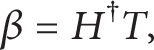
where H_† is the Moore-Penrose generalized inverse of the hidden layer matrix.

The special solution β∘ = H_†T is actually one of the least-squares solutions of a general linear system Hβ = T, and the smallest training error can be reached by the special solution ∥Hβ∘ − T∥ = ∥HH_†T − T∥ = min⁡_β∥Hβ − T∥ which could minimize training error. Moreover, the special solution β∘ = H_†T has the smallest norm among all the least squares solutions of Hβ − T which could calculate the smallest norm of weights. Thus, the Moore-Penrose generalized inverse of the hidden layer matrix is the key to acquire the performance of ELM. The detailed properties of Moore-Penrose generalized inverse matrix could be seen in the literature [27]

The structure of an ELM can be illustrated in Figure 1.

Figure 1:

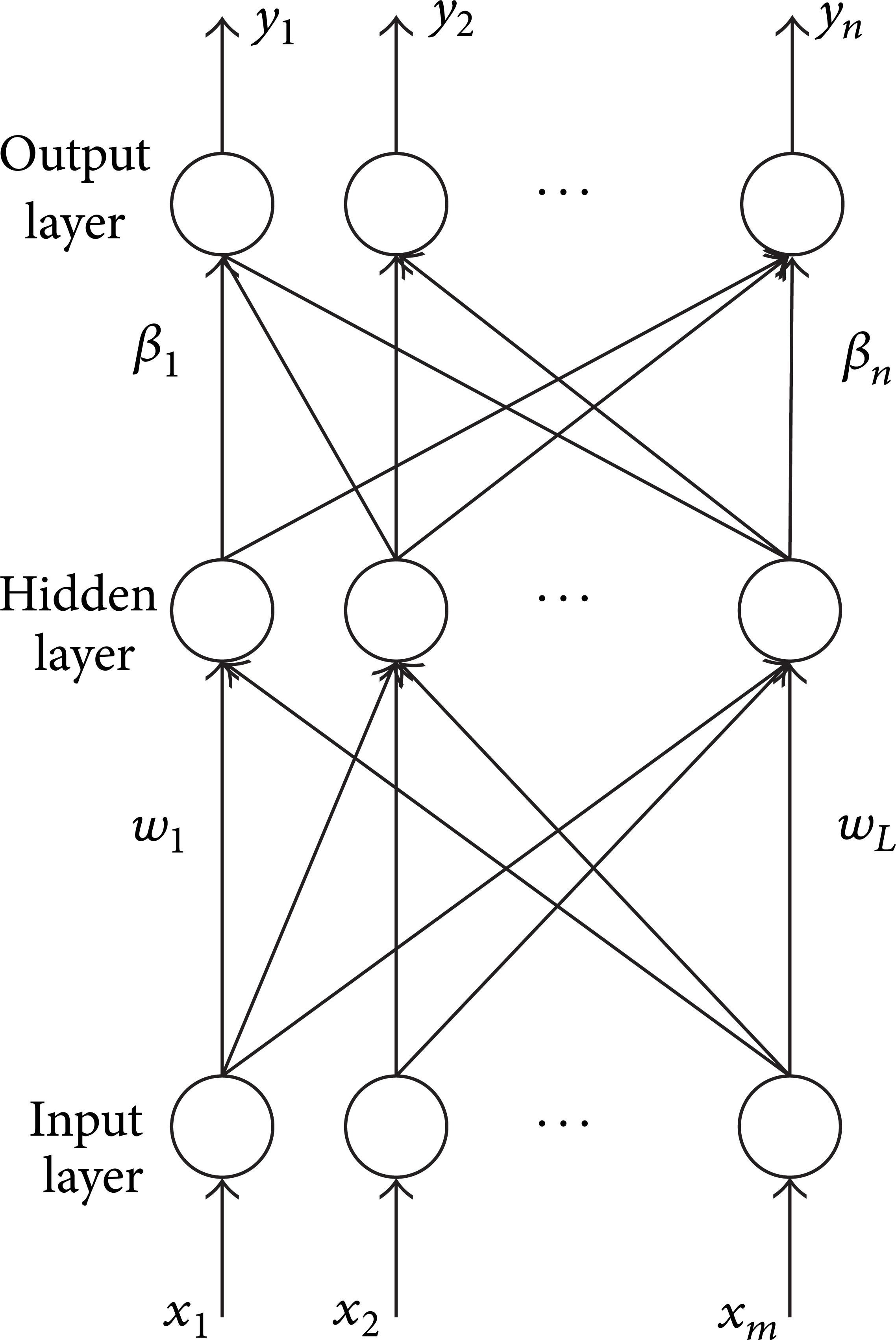
The structure of ELM.

3.2. Artificial Bee Colony (ABC) Algorithm

Artificial bee colony (ABC) was proposed in recent years as a novel biological-inspired optimization algorithm method [28]. In the ABC algorithm, the potential solution is represented by using the food source position, and the fitness of the associated solution is represented by the nectar amount of a food source. The ABC algorithm consists of three types of bees: employed bee, onlooker bee, and scout bees.

The employed bee is the mutation stage. In the employed bee stage, a new candidate solution is firstly given by the following solution search equation:

v_{i j} = x_{i j} + ϕ_{i j} (x_{i j} - x_{k j}),

(11)

where x_ij and v_ij denote the original and modified jth element of x_i, respectively, and j is a random index. x_k denotes another solution selected randomly from the population and k≠j; ϕ_ij is a uniform random number in [− 1, 1]. When the update process is completed, a greedy selection is done between x_i and v_i.

The onlooker bee is the solutions selection stage using the roulette strategy. The main distinction between the employed bee stage and the onlooker bee stage is that each solution in the employed bee stage could be updated, but only the selected solutions have the chance to be updated in the onlooker stage. An onlooker bee chooses a food source depending on the probability value associated with that food source p_i, calculated by the following expression (6):

p_{i} = \frac{{fit}_{i}}{\sum_{n = 1}^{SN} {fit}_{n}},

(12)

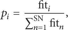
where fit_i denotes the fitness value of ith food source and SN denotes the number of food sources.

At last, the scout stage disposes an inactive solution which does not change over a certain number of generations and replaces it by a new randomly generated solution.

x_{i}^{j} = x_{\min}^{j} + rand [0,1] (x_{\max}^{j} - x_{\min}^{j}) .

(13)

3.3. Ensemble Optimal Extreme Learning Machine

In this section, we proposed a novel classification model called EO-ELM and applied multifault classification. The EO-ELM utilized the ABC evolutionary algorithm which is used to optimize the node weights and bias of ELM. When several ELMs have been trained well, the major voting method is employed to construct the ensemble classifier. Combine the EO-ELM and IMPE proposed in the above section. The complete process of the proposed fault diagnosis method is given in the following steps.

Step 1. The original vibration signal of rolling element bearing is acquired by data acquisition system and decomposed with EEMD. Then all the IMFs and the residue were obtained and the first m IMFs were chosen to calculate the feature vector when they contain the 95% total accumulation energy.

Step 2. The first m IMFs are calculated as (1)–(3), and the PE of each IMF is calculated as (4)–(7). Finally, the feature matrix is acquired by calculating all the IMPEs of subsignals.

Step 3. Given an ensemble of N ELMs with the same input node and hidden node number, divide the dataset into the train part and test part as predefined percentage, and set the ELM model index n = 1.

Step 4. Initialize the control parameter of ABC, such as the maximum cycle number (MCN), the number of food position, and randomly generate weights and bias as the candidate solutions of ABC in the search space. And perform the nth ELM model training process on the bearing dataset.

At the employed bee stage, the population is evaluated by calculating the cross-validation rate of nth ELM on train dataset and the new solutions for employed bees are generated by using (11).

Produce the new solutions for the onlookers and evaluate them with applying the greedy selection process.

Determine the abandoned solution for the scout bee, if it exists, and replace it with a new randomly produced solution x_i.

Memorize the best solution achieved so far.

Repeat the steps (a)~(d) until the iteration number is more than the maximum cycle number. Then the optimal parameter is employed to construct the nth ELM model.

Step 5. When all the ELMs have been optimized by the ABC algorithm successfully, it can be used to identify the different fault patterns of test samples rolling bearings. We use the major voting method to ensemble these ELMs, which is the final output of the EOS-ELM.

The flow chart of the proposed method is shown in Figure 2.

Figure 2:

The flow chart of the proposed diagnosis method.

4. Experimental Results

4.1. Experiment Setup

In this experiment, the EO-ELM algorithm was applied on fault diagnosis of rolling element bearing. The experiment data was kindly provided by Case Western Reserve University (CWRU) and has been widely considered as a benchmark fault diagnosis problem [29]. As shown in Figure 3, the rolling element bearings test stand consists of an induction motor supported in Figure 3(a), a torque transducer/encoder at the center, and a dynamometer in Figure 3(b). The detailed information of bearing test stand could be seen in this literature [30 –32]. All the simulation programs were run in MATLAB 7.5 environments on a computer with Intel Core 2.5 GHz CPU and 2 G RAM.

Figure 3:

The test rig.

4.2. Result and Analysis

The vibration signal with 0.007in, 0.014in, and 0.021in defect sizes at no motor load condition has been selected for this study. This paper utilized the data which was collected at 48000 Hz under 0 hp load. Each signal was divided to 118 pieces, and the length of each divided signal was 4096 data points. Figure 4 shows nine typical fault signals including outer raceway fault, inner raceway fault, and rolling element fault with different defect sizes.

Figure 4:

The waveform of different faults: (a) ball with 0.007in, (b) ball with 0.014in, (c) ball with 0.021in, (d) inner race with 0.007in, (e) inner race with 0.014in, (f) inner race with 0.021in, (g) outer race with 0.007in (h), outer race with 0.014in, (i) outer race with 0.021in.

Each subsignal was decomposed by EEMD. According to the literatures [12], the ensemble number of EEMD is set to 100 and the amplitude of the added white noise is 0.2. After analyzing the IMFs decomposed by EEMD, it was found that the first 12 IMFs almost contain all the energy of the original signal. Figure 5 shows the first 12 IMFs of EEMD decomposition results for the inner race fault signal. The IMPE of these IMFs was calculated in each sample. The IMPE has two important parameter to define, the embed dimension and the time lay. According to the literature [18], the embed dimension is set to 5 and the time lay is set to 3 in this experiment. Then, the 9 fault conditions which contained 1065 samples with 12 dimensions were acquired to construct IMPE feature matrix. Figure 6 shows the three-dimension map of IMPE feature matrix by PCA for all the samples. In Figure 6, the inner race fault, ball fault, and outer race fault are denoted by using the “IR,” “B,” and “OR,” respectively. And the different fault defect size is denoted by using the “007,” “014,” and “021”. It could be clearly seen that the different fault conditions can be clearly classified relatively.

Figure 5:

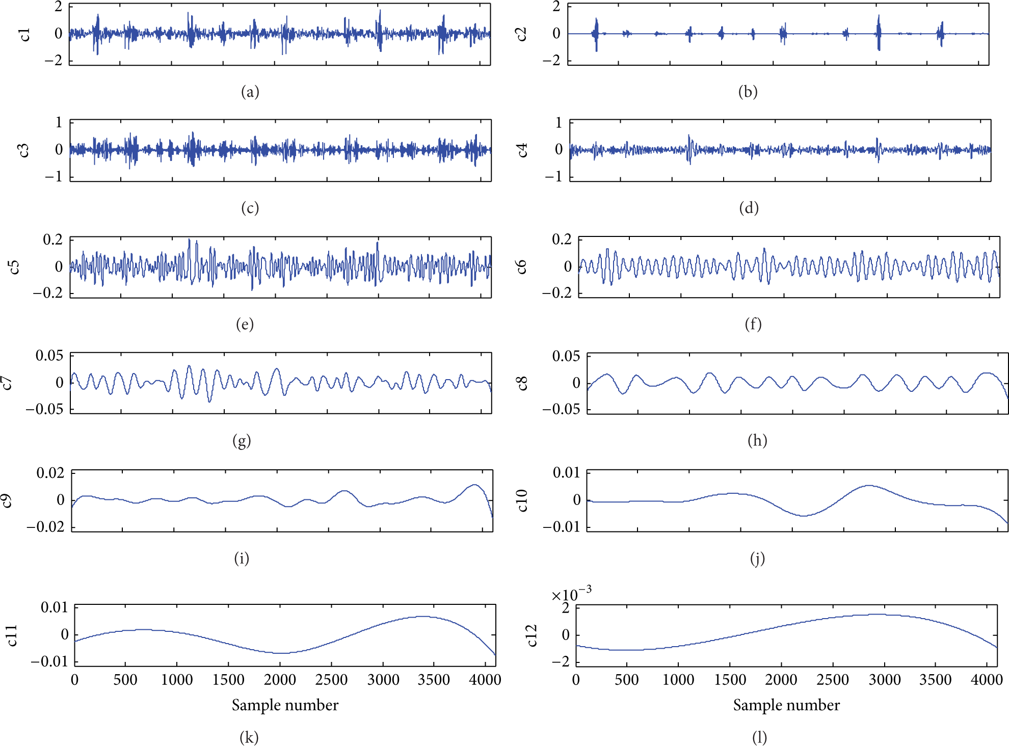
The decomposed results of the inner race fault signal using EEMD.

Figure 6:

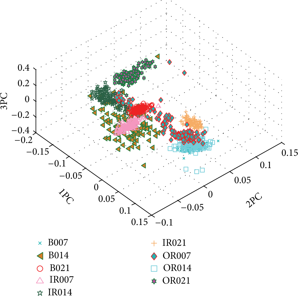
The three dimensions map of different IMPE feature fault sample points by PCA.

To illustrate the proposed approach, three group experiments were carried out to evaluate the performance of the proposed method based on the experimental data obtained from the above-mentioned tests. The detailed experiments are as follows. Case 1 has three bearing fault types which are inner race fault, outer race fault, and ball fault with two levels of severity for each fault type, 0.007in and 0.014in, which are considered as the six classes of pattern recognition problem. Case 2 has similar setting as Case 1, except that the two levels of severity are 0.007in and 0.021in. Case 3 contains all nine classes fault. In each experiment, the dataset was sorted randomly and selected partly as training data, and the rest were selected as testing data. The detailed description of each experiment is shown in Table 1.

Table 1:

The detailed setting of the experiments.

Case	Fault label	Operating condition	Label of classification	Defect size (inches)	The number of training samples	The number of testing samples

1	IR007	Inner race	1	0.007	500	209
	IR014	Inner race	2	0.014
	OR007	Outer race	3	0.007
	OR014	Outer race	4	0.014
	B007	Ball	5	0.007
	B014	Ball	6	0.014

2	IR007	Inner race	1	0.007	500	210
	IR021	Inner race	2	0.021
	OR007	Outer race	3	0.007
	OR021	Outer race	4	0.021
	B007	Ball	5	0.007
	B021	Ball	6	0.021

3	IR007	Inner race	1	0.007	800	265
	IR014	Inner race	2	0.014
	IR021	Inner race	3	0.021
	OR007	Outer race	4	0.007
	OR014	Outer race	5	0.014
	OR021	Outer race	6	0.021
	B007	Ball	7	0.007
	B014	Ball	8	0.014
	B021	Ball	9	0.021

In this paper, we experimentally evaluated the performance of features extracted by IMPE. The traditional energy entropy method was employed to compare with the proposed IMPE. Moreover, the features matrixes extracted by two methods were classified by EO-ELM original ELM, EE-ELM, and DE-ELM for bearing fault diagnosis. Each experiment was repeated 30 times, and the average test accuracy and standard derivation of each method could be seen in Table 2.

Table 2:

Comparison result of different algorithms.

	IMPE			Energy entropy
	Case 1	Case 2	Case 3	Case 1	Case 2	Case 3

ELM	95.02 ± 0.78	97.27 ± 0.89	92.94 ± 1.30	90.25 ± 1.87	92.93 ± 1.04	90.76 ± 1.27
DE-ELM	95.86 ± 0.78	97.68 ± 1.26	94.14 ± 2.08	93.10 ± 2.16	97.05 ± 1.31	91.88 ± 1.23
EELM	95.88 ± 0.42	98.27 ± 0.47	93.84 ± 0.98	92.55 ± 1.01	93.72 ± 0.63	91.35 ± 0.82
EO-ELM	96.80 ± 0.41	98.85 ± 0.68	95.66 ± 0.92	94.33 ± 1.45	98.10 ± 0.64	92.35 ± 1.17

It can be found that the classification rates of all the three classifiers using IMPE based features have all achieved better performances than the traditional energy entropy. Furthermore, among the four classifiers, the EO-ELM has the best classification accuracy and the smallest standard derivation which means that the EO-ELM has the best general ability and robustness performance. The classification result of the EO-ELM was presented in Figure 7. In Figure 7, it is shown that the proposed approach can reliably recognize different fault categories and severities.

Figure 7:

Classification result using the EO-ELM: (a) Case 1 with six fault types, (b) Case 2 with six fault types, (c) Case 3 with nine fault types.

4.3. Discussion

Compared to the traditional energy entropy, the IMPE has better performance in three diagnosis experiments. It could be concluded that the IMPE can easily and clearly classify the different fault working conditions of rolling element bearing.

The classification results in three bearing fault diagnosis experiments prove that the proposed method based on EO-ELM obtains relatively good improvement in identification accuracy and generalization performance. The classification accuracies of EO-ELM method are better than the original ELM, EE-ELM, and DE-ELM. The mean accuracy result of IMPE-EO-ELM is 95.66 in Case 3, but the ELM and E-ELM are only 92.94 and 93.84. It shows that the EO-ELM outperforms the other algorithm and has better generalization performance when the class label number is especially large, which has much more practical meaning in the engineering application. Furthermore, the standard variance of EO-ELM diagnosis result is 0.41, 0.68, and 0.92 which are almost minimum value among the results of these algorithms. Thus it is indicated that the proposed method also has better robustness to guarantee the credible diagnosis result.

In the future research, a higher efficient model of EO-ELM will be made beyond current levels, and efforts will be made towards optimal fault feature subset selection.

5. Conclusion

Although recently various algorithms have been tried out for solving bearing fault diagnosis problems of bearing, it is rare to see the classification ability to classify the faults and severity. Taking into consideration this point, a novel bearing fault diagnosis method named IMPE-EO-ELM was proposed in this paper. In the proposed algorithm, the original vibration signals were decomposed into a number of IMFs by EEMD adaptively and the permutation entropy was utilized to extract the nonlinear characteristic information of each IMF and generate the fault feature matrix. The proposed method is tested in three experiments with different fault types and severities. From the results obtained, we may conclude that IMPE technique could extract nonlinear dynamic feature of bearing vibration signal and is sensitive to the variations of fault severity. And combining the merit of evolutionary ELM and the ensemble ELM, a new variant of ELM was proposed to identify the fault type and severity which employed the ABC algorithm to select the weights and bias of server ELMs and utilized the major voting ensemble classification method to determine the final output of these ELMs. The result shows that the proposed algorithm has better classification performance and robustness than the original ELM, EE-ELM, and DE-ELM. Furthermore, the method could be suited well for tackling other similar classification problems in the future.

Conflict of Interests

All of the authors do not have any direct financial relation with the commercial identities mentioned in this paper.

Footnotes

Acknowledgments

The authors would like to thank the Western Reserve University for providing experimental data. In addition, the work described in this paper is supported by the National Natural Science Foundation of China under Grant no. 51239004, the National Natural Science Foundation of China under Grant no. 51079057, and the research funds of University and college Ph.D. Discipline of China (no. 20100142110012).

References

Randall

R. B.

and Antoni

, “Rolling element bearing diagnostics—a tutorial,” Mechanical Systems and Signal Processing, vol. 25, no. 2, pp. 485–520, 2011.

William

P. E.

and Hoffman

M. W.

, “Identification of bearing faults using time domain zero-crossings,” Mechanical Systems and Signal Processing, vol. 25, no. 8, pp. 3078–3088, 2011.

Wang

Z. W.

Zhu

Z. C.

Zhou

G. B.

, and Chen

G. A.

, “Design of online monitoring and fault diagnosis system for belt conveyors based on wavelet packet decomposition and support vector machine,” Advances in Mechanical Engineering, vol. 2013, Article ID 797183, 10 pages, 2013.

Lim

M. H.

and Leong

M. S.

, “Detection of early faults in rotating machinery based on wavelet analysis,” Advances in Mechanical Engineering, vol. 2013, Article ID 625863, 8 pages, 2013.

Miao

Z. H.

Zhou

G. X.

Wang

X. H.

, and He

C. X.

, “Study on immune relevant vector machine based intelligent fault detection and diagnosis algorithm,” Advances in Mechanical Engineering, vol. 2013, Article ID 548248, 8 pages, 2013.

Huang

N. E.

Shen

Long

S. R.

, “The empirical mode decomposition and the Hilbert spectrum for nonlinear and non-stationary time series analysis,” Proceedings of the Royal Society A: Mathematical, Physical and Engineering Sciences, vol. 454, no. 1971, pp. 903–995, 1998.

Ricci

and Pennacchi

, “Diagnostics of gear faults based on EMD and automatic selection of intrinsic mode functions,” Mechanical Systems and Signal Processing, vol. 25, no. 3, pp. 821–838, 2011.

Huang

N. E.

and Wu

, “Ensemble empirical mode decomposition: a noise-assisted data analysis method,” Advances in Adaptive Data Analysis, vol. 1, pp. 1–41, 2009.

Lei

Y. G.

Lin

Z. J.

, and Zuo

M. J.

, “A review on empirical mode decomposition in fault diagnosis of rotating machinery,” Mechanical Systems and Signal Processing, vol. 35, no. 1–2, pp. 108–126, 2013.

10.

Liu

Chen

Zhou

Z. D.

, and Wei

, “Fault diagnosis of rolling bearing based on wavelet package transform and ensemble empirical mode decomposition,” Advances in Mechanical Engineering, vol. 2013, Article ID 792584, 6 pages, 2013.

11.

Lei

Zuo

, and Hoseini

, “The use of ensemble empirical mode decomposition to improve bispectral analysis for fault detection in rotating machinery,” Proceedings of the Institution of Mechanical Engineers C: Journal of Mechanical Engineering Science, vol. 224, no. 8, pp. 1759–1769, 2010.

12.

Lei

Y. G.

Z. J.

, and Zi

Y. Y.

, “Application of the EEMD method to rotor fault diagnosis of rotating machinery,” Mechanical Systems and Signal Processing, vol. 23, no. 4, pp. 1327–1338, 2009.

13.

Zhang

and Zhou

, “Multi-fault diagnosis for rolling element bearings based on ensemble empirical mode decomposition and optimized support vector machines,” Mechanical Systems and Signal Processing, vol. 41, no. 1–2, pp. 127–140, 2013.

14.

Guo

Tse

P. W.

, and Djordjevich

, “Faulty bearing signal recovery from large noise using a hybrid method based on spectral kurtosis and ensemble empirical mode decomposition,” Measurement, vol. 45, no. 5, pp. 1308–1322, 2012.

15.

Yan

R. Q.

and Gao

R. X.

, “Approximate entropy as a diagnostic tool for machine health monitoring,” Mechanical Systems and Signal Processing, vol. 21, no. 2, pp. 824–839, 2007.

16.

Zhang

Xiong

Liu

Zou

, and Guo

, “Bearing fault diagnosis using multi-scale entropy and adaptive neuro-fuzzy inference,” Expert Systems with Applications, vol. 37, no. 8, pp. 6077–6085, 2010.

17.

Nicolaou

and Georgiou

, “Detection of epileptic electroencephalogram based on permutation entropy and support vector machines,” Expert Systems with Applications, vol. 39, no. 1, pp. 202–209, 2012.

18.

Yan

R. Q.

Liu

Y. B.

, and Gao

R. X.

, “Permutation entropy: a nonlinear statistical measure for status characterization of rotary machines,” Mechanical Systems and Signal Processing, vol. 29, pp. 474–484, 2012.

19.

Amoud

Snoussi

Hewson

Doussot

, and Duchene

, “Intrinsic mode entropy for nonlinear discriminant analysis,” IEEE Signal Processing Letters, vol. 14, no. 5, pp. 297–300, 2007.

20.

Wang

Y. G.

Cao

F. L.

, and Yuan

Y. B.

, “A study on effectiveness of extreme learning machine,” Neurocomputing, vol. 74, no. 16, pp. 2483–2490, 2011.

21.

Liu

X. Y.

Gao

C. H.

, and Li

, “A comparative analysis of support vector machines and extreme learning machines,” Neural Networks, vol. 33, pp. 58–66, 2012.

22.

Han

Yao

H. F.

, and Ling

Q. H.

, “An improved evolutionary extreme learning machine based on particle swarm optimization,” Neurocomputing, vol. 116, pp. 87–93, 2012.

23.

Cao

J. W.

Lin

Z. P.

, and Huang

G. B.

, “Self-adaptive evolutionary extreme learning machine,” Neural Processing Letters, vol. 36, no. 3, pp. 285–305, 2012.

24.

Xiao

Zhou

Xiao

Zhang

, and Zhu

, “Multi-fault classification based on the two-stage evolutionary extreme learning machine and improved artificial bee colony algorithm,” Proceedings of the Institution of Mechanical Engineers C: Journal of Mechanical Engineering Science, 2013.

25.

Liu

and Wang

, “Ensemble based extreme learning machine,” IEEE Signal Processing Letters, vol. 17, no. 8, pp. 754–757, 2010.

26.

Huang

G. B.

Zhou

H. M.

Ding

X. J.

, and Zhang

, “Extreme learning machine for regression and multiclass classification,” IEEE Transactions on Systems, Man, and Cybernetics B: Cybernetics, vol. 42, no. 2, pp. 513–529, 2012.

27.

Huang

G.-B.

Zhu

Q.-Y.

, and Siew

C.-K.

, “Extreme learning machine: theory and applications,” Neurocomputing, vol. 70, no. 1–3, pp. 489–501, 2006.

28.

Karaboga

and Akay

, “A comparative study of artificial bee colony algorithm,” Applied Mathematics and Computation, vol. 214, no. 1, pp. 108–132, 2009.

29.

Wang

Y. J.

Kang

S. Q.

Jiang

Y. C.

Yang

G. X.

Song

L. X.

, and Mikulovich

V. I.

, “Classification of fault location and the degree of performance degradation of a rolling bearing based on an improved hyper-sphere-structured multi-class support vector machine,” Mechanical Systems and Signal Processing, vol. 29, pp. 404–414, 2012.

30.

Jiang

Xuan

, and Shi

, “Feature extraction based on semi-supervised kernel Marginal Fisher analysis and its application in bearing fault diagnosis,” Mechanical Systems and Signal Processing, vol. 41, no. 1–2, pp. 113–126, 2013.

31.

Zhu

Song

, and Xue

, “A roller bearing fault diagnosis method based on hierarchical entropy and support vector machine with particle swarm optimization algorithm,” Measurement, vol. 47, pp. 669–675, 2014.

32.

Loparo

, Bearings Vibration Data Set, Case Western Reserve University, Cleveland, Ohio, USA, 2003.

Multifault Diagnosis for Rolling Element Bearings Based on Intrinsic Mode Permutation Entropy and Ensemble Optimal Extreme Learning Machine

Abstract

1. Introduction

2. Intrinsic Mode Permutation Entropy

2.1. A Brief View of EEMD

2.2. Permutation Entropy and IMPE

3. Ensemble Optimal Extreme Learning Machine

3.1. Brief Introduction of Extreme Learning Machine

3.2. Artificial Bee Colony (ABC) Algorithm

3.3. Ensemble Optimal Extreme Learning Machine

4. Experimental Results

4.1. Experiment Setup

4.2. Result and Analysis

4.3. Discussion

5. Conclusion

Conflict of Interests

Footnotes

Acknowledgments

References