
Abstract
For a wireless sensor network (WSN) with a large number of inexpensive sensor nodes, energy efficiency is the major concern in designing network structure and related algorithms. If network collects sensor data using mobile sinks, object tracking mechanism must consider the energy efficiency of sensor nodes in the networks as a whole. Recently research works on WSNs with mobile sinks apply prediction techniques for sink tracking in order to improve tracking precision while keeping the number of active nodes to the minimum. In this paper, we analyze existing works for sink tracking in WSN and propose P-LEACH that is cluster-based prediction technique for WSN with mobile sinks. Simulation results show that P-LEACH performs better than previous techniques in terms of energy saving of sensor nodes and data transmission performance.
1. Introduction
Recent advancement in electronics technology allowed designers to develop low-cost wireless sensor networks with thousands of small and cheap sensors. These sensor networks are widely used in many application areas such as military, environmental, health, and security areas. Despite good potential applicability of WSN, its design has many constraints: limited battery life, low computational power, and limited transmission range of sensor nodes. In particular, a sensor has limited battery life and this battery cannot be replaced due to the area of deployment; networks lifetime depends on the battery capacity of sensors deployed.
The idea of sensor data collection using mobile sinks has recently been proposed as an alternative solution for applications that need to collect real-time data on the spot or that require high data rate. Research issues on WSNs with mobile sinks are two: (a) collection and transmission of sensors’ data to mobile sinks and (b) effective sink tracking. Studies for target tracking are categorized by three techniques: tree-based, cluster-based, and prediction-based techniques. They try to solve the common problem in the WSNs with mobile sinks: how to reduce the number of active sensors that should stay awake for tracking of moving sinks and how to reduce the energy consumption of managing sensors.
In this paper, we analyze three typical object tracking techniques: STUN (scalable tracking using networked sensors) [1] for tree-based technique, acoustic target tracking [2] for cluster-based technique, and DMSTA (dynamic distributed tree-based tracking algorithm) [3] for prediction-based technique. We then propose the P-LEACH (partition-LEACH) to solve the major problem in the WSNs with mobile sink. The basic idea of P-LEACH is as follows: it achieved data transmission efficiency by making all clusters circle shaped; saved energy of sensors by partitioning a cluster into four independent areas, thus distributing the roles of a managing sensor into four gate nodes; and could efficiently track mobile sink using distances between four gate nodes and the mobile sink.
The organization of this paper is as follows. In Section 2, we analyzed three typical target tracking techniques in wireless sensor networks: STUN, acoustic target tracking, and DMSTA. In Section 3, we describe the proposed technique P-LEACH in detail: the components of P-LEACH and their workings to track mobile sinks. We compared P-LEACH with convention technique LEACH in Section 4. In Section 5, we performed simulation on the above three techniques and P-LEACH and analyzed the results. Finally, Section 6 offers concluding remarks.
2. Related Works
In this section, we describe existing works in two areas: (a) general architecture and routing protocols in wireless sensor networks and (b) techniques to track moving objects.
2.1. Hierarchical Architecture and Routing Protocols
Energy efficient routing protocol is the major concern in WSNs. A number of routing protocols have been proposed for WSN. Among them, hierarchical routing protocols provide maximum energy efficiency. The whole network is divided into multiple clusters. A node is selected as a cluster head (CH). CH is the only node that can communicate with base station. This significantly reduces routing overhead of normal nodes because normal nodes transmit their data to CH only.
LEACH (low energy adaptive clustering hierarchy) is considered as a basic energy efficient hierarchical protocol [4–7]. In cluster structure, CH spends most energy and if it remains as CH permanently, it dies quickly in case of static clustering. LEACH tackles this problem by randomizing rotation of CH to save the battery life of individual nodes. This, in turn, maximizes lifetime of network nodes. Quite a few extended-LEACH routing protocols have been proposed since then. Reference [7] presents recent survey results on energy efficient hierarchical routing protocols, developed from conventional LEACH protocol.
Recently, data collection in sensor networks using mobile sinks has been investigated to improve energy performance at the cost of collection delay. Reference [8] is a recent survey paper that presents a modeling framework for characterizing the feasibility and impacts of multihop packet routing in sensor network with mobile sinks. Reference [9] proposes MWST (minimum Wiener index spanning tree) as a routing topology that is suitable for sensor networks with multiple mobile sinks.
2.2. Tracking of Moving Objects
Moving object tracking using WSN has received considerable attention in recent years. Existing works on moving object tracking in wireless sensor networks have two related areas: those on the transmission and collection of data for the renewal of moving object's positions and those on the least activation of sensor nodes necessary to track the object. Proposed solutions on object tracking techniques can be mainly classified into three schemes: tree-based tracking, cluster-based tracking, and prediction-based tracking techniques [10–12].
2.2.1. Tree-Based Object Tracking
In tree-based object tracking, nodes in a network are organized in a hierarchical tree or represented as a graph in which vertices represent sensor nodes and edges are links between nodes. Examples of tree-based methods are STUN [1], DCTC (dynamic convoy tree-based collaboration) [13], and MWST [9].
In STUN, the leaf nodes of tree are used for tracking the moving object and then sending collected data to the root (i.e., the sink) through intermediate nodes. It can track multiple objects simultaneously. DCTC uses a tree structure called convoy to track objects. Tracking is performed through the collaboration of multiple sensor nodes. The tree is dynamically configured to add and prune nodes when the target moves. Sensor nodes whose distance from the target is above a specific value are eliminated from the tree, and sensor nodes near the object are added to the tree. MWST simplified tree organization using a spanning tree. This technique is designed to track moving objects using small hop-counts.
The tree structure is effective in reducing communication costs by eliminating the transmission of duplicated message in a network. Since objects are moving randomly in a network, tree structure is easy to be broken and thus the cost of maintaining a tree structure could be very high.
2.2.2. Cluster-Based Object Tracking
The cluster-based techniques organize the network of sensors by clusters in order to support collaborative data processing. A cluster has a cluster head (CH) node and member nodes. CH is the manager of a cluster that controls its sensor nodes for object tracking and acts as the gateway for data transmission to the sink from its sensor nodes. To be energy efficient in object tracking, only some sensor nodes within a cluster become active. Examples of cluster-based techniques are acoustic target tracking technique [2], ADCT (adaptive dynamic cluster-based tracking) [14], and CMSE (cluster-based mobile sink exploration) [15].
Acoustic target tracking technique uses a fixed backbone of high-capacity sensor nodes that acts as CHs. The CHs become in active state when they sense signal strength (of target) beyond a certain value that is established in advance. The activated CHs wake up neighbor sensors and construct dynamic clusters. ADCT uses the optimal choice mechanism and dynamic cluster-based approach to achieve a good tracking quality and energy efficiency by optimally choosing the nodes that participate in tracking and minimizing communication overhead and thus prolongs the lifetime of the whole sensor network. In CMSE, a CH informs its senor nodes of the direction information of mobile sink, if it sensed moving object. With the direction information, sensor nodes can send collected data to the mobile sink in a shortest path by sending directly to the nodes near the sink.
2.2.3. Predication-Based Object Tracking
Prediction-based techniques reduce energy consumption of sensor network by making only a small part of sensors active while tracking targets. These schemes are built on the tree-based or cluster-based schemes. They predict the next location of target objects using a prediction algorithm. Then they select some nodes that are near this predicted location for tracking and other nodes remain in sleep mode for energy saving. Examples are DPR (dual prediction-based reporting) [16] and DMSTA [3].
In DPR, both sensor nodes and the base station predict the future movements of the mobile objects. Transmissions of sensor readings are avoided as long as the predictions are consistent with the real object movements. DPR reduces energy consumption by avoiding long-distance transmission between the base stations and sensor nodes. In the prediction-based techniques, it is necessary to predict more accurately the direction of targets, since the reliability of object tracking depends on the prediction precision. Moreover, tracking failure occurs more frequently in this technique because some prediction error is inevitable.
DMSTA is a dynamic, distributed tree-based tracking algorithm for very fast-moving targets in WSNs. Its aim is to decrease the miss ratio and the energy consumption while tracking objects that move in high speed. In this technique, sensor nodes up to n-hops away from the predicted trajectories of moving objects are activated in order to reduce the probability of failure. The node closest to the target becomes a new root of tree and expanded. Figure 1 shows the activation of sensor nodes for tracking moving objects.
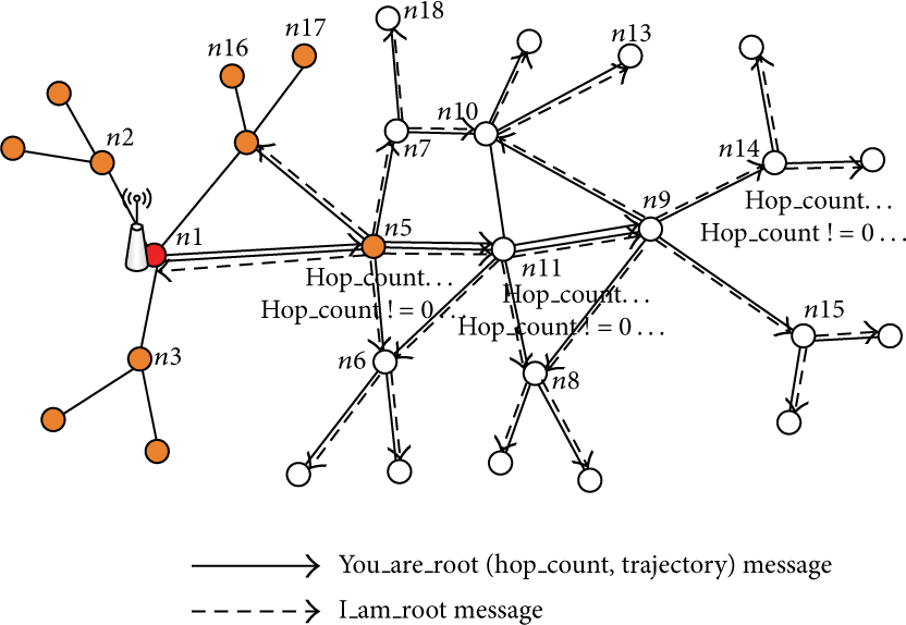
Tree-expansion in DMSTA to track a moving object.
While DMSTA is effective in tracking the fast-moving object, energy consumption for tree construction and reconstruction according to the movement of the object is still very high. Also, the strategy based on the hop-count is much influenced by the density of sensor nodes. If tracking fails, the restoration process spends a lot of energy because all nodes that are n-hop away from the root are activated.
3. P-LEACH: Concepts and Operations
P-LEACH is a cluster-based prediction technique and an improvement of LEACH to handle wireless sensor network with mobile sinks. In this section, we describe the P-LEACH in detail: concepts in P-LEACH and components of the network with their operations for tracking and data transmission.
In P-LEACH, the wireless sensor network consists of equal-sized clusters called partition clusters (PCs). A PC is a circle area of radius r around the cluster center node. Initially, hundreds or thousands of sensors are deployed in the fields. PCs are constructed as follows: a sensor node with the most battery capacity becomes the cluster center of the first PC. The other PCs in the network are formed around the first PC. They are all in the same shape, that is, circles of the same radius r. A sensor node in the center of each PC becomes the cluster center.
Figure 2 shows three conceptual regions in P-LEACH network. Region 1 in the figure is a PC, cluster structure in P-LEACH. Region 2 shows a communication quadrangle (CQ), which is the collaboration structure among four adjacent PCs. Region 3 shows a structure with four PCs in a network.

Three conceptual regions in P-LEACH network.
3.1. Partition Cluster (PC)
A PC is a circle area with radius r and has sensor nodes deployed within the circle. Among the sensors nodes, some are used for special purposes. Every PC has one cluster center (CC) node, four partition nodes (Pns), and four gate nodes (Gns). Figure 3 shows the details of a PC. In the figure, ordinary sensor nodes are not shown. Sensor nodes deployed in the field are to collect and transmit specific data in the field. All sensors have an identical r-value, a length value, which is used in selecting a CC node, Pns, and Gns. The CC node is the sensor node located in the center of a PC; four Pns are located on the border line of the PC circle; and four Gns play the role of both delivering data collected from the sensor nodes and monitoring the presence of a mobile sink.

Structure of a partition cluster (PC).
3.1.1. Sensor Nodes
Sensor nodes are to collect data in the field deployed. They also participate in selecting candidates for CC, Pn, and Gn. At the initial installation, every sensor node has a sensor ID with an r-value and a P value. The ID of a sensor node is made up with the group ID that identifies all the sensors deployed and a serial number (SN). r-value represents the circle radius of PC and is used in selecting candidates for Pn. P value is the hypotenuse of a right-angled triangle and is used to determine four Pns.
Ordinary sensors stay in the sleeping state to save energy if there is no event occurring within PC or no mobile sink around. The sleeping mode is called deep sleep, in which sensors minimize their energy consumption. See Figure 4.
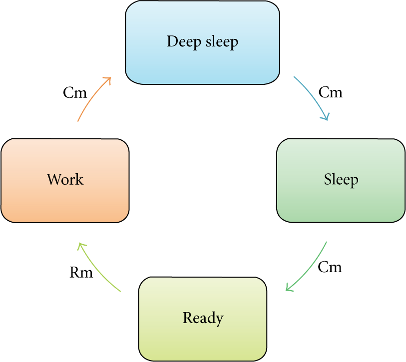
Changes in PC states.
When a Gn detects a mobile sink, it sends a condition message (Cm) to three other Gns and they change their states from deep sleep to sleep. In the sleep mode, only Gns are awake and monitor the mobile sink's movement. Gn changes its state to the ready state if the mobile sink is coming right over the PC. Gn in the ready state waits for a resolution message (Rm) from another Gn in the work state. The message is issued if the mobile sink leaves the PC. Gn in the ready state changes its state to the work state, if Rm is received. In the work state, all sensors nodes in the PC are awake.
Ordinary sensors are supposed to deliver collected data to the mobile sink through one of the Gns in the cluster. Sensors continue data transmission until the mobile sink leaves PC and changes its state from work to deep sleep when transmission ends.
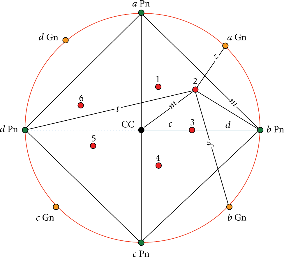
3.1.2. Cluster Center (CC) and Selection of Pn
CC is a sensor node selected only to construct a PC structure. Initially, a candidate CC becomes a temporary CC (TCC). The sensor that has the least SN number (A, 1) is selected as TCC. See Figure 5. The TCC collects information on sensors at r-distance from the center. Among the sensors, one that is the closest to the r-distance (A, 11) is selected and named a Pn. The sensors b and d are selected next as Pns. Both are p-distant from a and r-distant from CC. Finally, c is selected as another Pn of the PC. Those four Pns transmit their information to the TCC, and the TCC registers the information and changes its status to the CC.

Selection of four Pns of a PC.
3.1.3. Gate Node (Gn)
Gns play the role of collecting data from the four partitions and then transmitting them to the sink with some data manipulation if necessary. Gn is selected among the candidates Pns selected above. A Gn is located in the center of an arc connecting two adjacent Pns as shown in Figure 6. Gn q, for example, is selected as follows: point f is the middle point between Pn a and Pn b. Among candidate Pns, select point q that is on the straight line from the CC to f and k-distant from f, where value k satisfies the equation

Selection of four Gns.
3.1.4. Sensor Registration
Every sensor node in a PC should register its information to a Gn, and the Gn should check if the requesting node is in its partition. In our scheme, even though a PC has 4 partitions, we divide the PC into two halves, that is, (A~B~C) area and (A~D~C) area, in order to make the registration process fast and simple. See Figure 7. There are two Gns in each half. After determining one area that it belongs to, the sensor node decides which Gn is closer to it and performs registration to the Gn. For example, in the figure, sensor node 2 first identifies that it belongs to (A~B~C) half by computing the distances
Sensor registration.
3.1.5. Reselection of Managing Sensors
After initial deployment of P-LEACH sensor network, managing sensors, that is, CC, Pn, and Gn, would die earlier than ordinary sensor nodes because of their heavy workload. If one of the managing nodes dies, a sensor node closest to the dead node takes its role. Among the managing nodes, Gn consumes more energy and dies earlier than others. When a Gn dies, a new node close to the dead Gn takes up the role. If Gns die repeatedly, however, they should be newly selected using CC nodes and Pns.
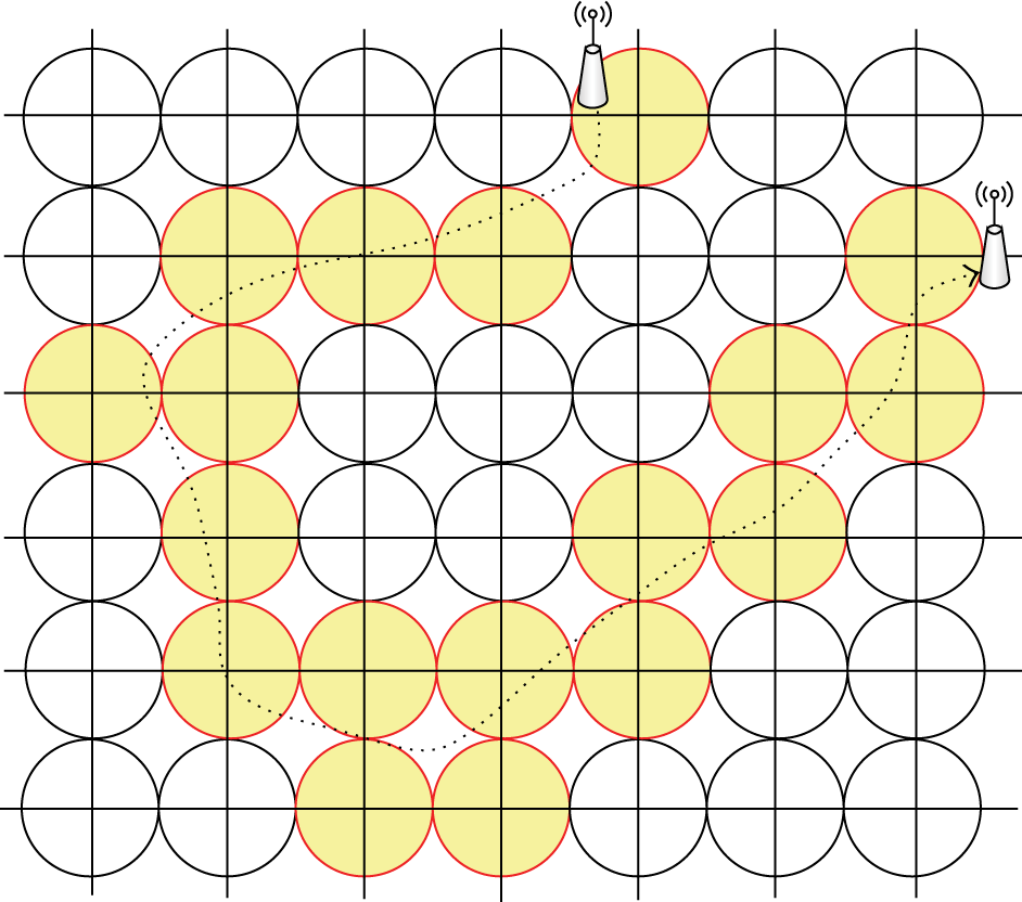
3.2. Communication Quadrangle (CQ)
In P-LEACH, the whole network consists of a number of PCs working together. Figure 8 shows a sensor network of 9 PCs. The network has 36 Pns and 36 Gns. We use the same Pn ID for two neighboring Pns of two adjacent PCs. Therefore 4 neighboring PCs form a common area having the same Pn ID, and the area is called CQ (communication quadrangle). In the figure, for example, the square c-b is a CQ formed by PCs A-B-D-E, and the square c-d is a CQ formed by PCs B-C-E-F. The common CQ ID is used as a managing ID in tracking the mobile sink. Four Gns in a CQ ID exchange information on the mobile sink and collaborate in its tracking.

Communication quadrangles in a P-LEACH network of 9 PCs.
3.3. Tracking Mobile Sinks
When a mobile sink is detected through one of four Gns, the Gn changes its state to work from sleep and continues tracking. If the distance between the Gn and the mobile sink goes over Mp (moving point), the Gn goes to deep sleep mode after transferring all tracking information to a Gn in the ready state. Figure 9 shows the calculation of the value Mp in a CQ.

State change of Gn using the value Mp.
Figure 10 shows how the states of 4 Gns are changing according to the location of mobile sink in a CQ. Gn D, after sensing a mobile sink within its area, informs Gns A, B, and C of the location of the mobile sink. Each Gn should decide its state by computing the value Mp.

Sate decision of Gn according to the location of mobile sink.
4. Comparison with LEACH
In this section, we compare P-LEACH with the conventional LEACH scheme in terms of data transmission efficiency and tracking efficiency. Here, “efficient” means consuming less energy of the network.
4.1. Data Transmission
Main differences between LEACH and P-LEACH scheme are both in the number of managing nodes and in the direction of data transmission from sensor nodes to mobile sink. In LEACH, one cluster head in a cluster handles transmission of data from all member sensors and tracking of mobile sink. In P-LEACH, four gate nodes in a cluster handle those tasks. Therefore, energy consumption of one cluster header in LEACH is distributed to 4 nodes and prolongs overall network lifetime.
As for the direction of data transmission, in LEACH data travels from outside to the center as in the path a in Figure 11 and is then transmitted back to the mobile sink, that is, path b in the figure. Thus, distance of data transmission in LEACH is as far as “

Data transmission in LEACH.
In case of P-LEACH, Gns are placed on the borderline (or outside) of PC. As in Figure 12, data travel time is

Data transmission in P-LEACH.
4.2. Mobile Sink Tracking
In this section, we analyze the clusters used to track a mobile sink. Figure 13 depicts regions necessary to track a mobile sink in P-LEACH scheme, and Figure 14 depicts the clusters necessary for the case of LEACH scheme. 33 regions are used in P-LEACH scheme, whereas 72 regions are used in LEACH scheme. In other words, P-LEACH uses less than 1/2 of the regions used in the case of LEACH. This means that energy consumption is less than half of that in the LEACH case.

Regions used to track a mobile sink (P-LEACH).
Regions used to track a mobile sink (LEACH).
5. Simulations
To validate the efficiency of P-LEACH, we performed simulations in terms of major characteristics of sensor network for three typical object tracking techniques (STUN, acoustic target tracking, and DMSTA) and P-LEACH. At the end, we summarized the results.
5.1. Parameter Setup
STUN, acoustic target tracking, DMSTA, and P-LEACH sensor networks were constructed using NS-2's SensorSim. Parameters setup for the simulation is summarized in Table 1.
Simulation parameters.
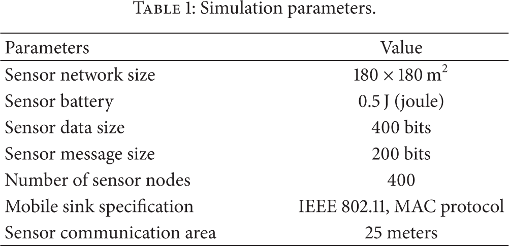
The acoustic target tracking consists of 9 clusters and 9 cluster headers; P-LEACH consists of 9 PCs, 36 Gns, and 36 Pns. The frequency of the measurement of mobile sink movement was randomly set up in STUN, and the DMSTA's extension trees were limited to 2n in the setup.
5.2. Energy Consumption
First, we measured the lifetime of sensor network in terms of dead sensors. In Figure 15, X coordinate represents time in hours and the Y coordinate is the number of dead sensors. The life span of each sensor network was measured by generating 100 events in one hour.

Number of dead sensors of networks in 24 hours.
The number of dead sensors increased due to message increase in the case of STUN and DMSTA. They increased rapidly after 15 hours since the measurement. This means that the amount of energy used to maintain the tree shape is great. Acoustic target tracking and P-LEACH both maintain clusters. The number of dead sensors was increased as cluster headers were replaced. We learned that managing sensors are dying uniformly 13 hours after the measurement in the case of P-LEACH. That is because most heavy load tasks in a cluster were managed by 4 Gns.
As for energy consumption of managing sensors for 24 hours, Figure 16 shows that P-LEACH consumed 20% of energy, STUN consumed 30%, acoustic target tracking consumed 60%, and the DMSTA consumed 20%.

Amounts of energy consumed by managing sensors in 24 hours.
Managing sensors in STUN and DMSTA use relatively small amount of energy because they do not manage the whole network. Acoustic target tracking uses more energy than P-LEACH because a single managing sensor deals with the whole network.
5.3. Data Transmission
For the effective transmission of data to mobile sink, it is necessary to predict the direction of mobile sink precisely, regardless of its speed.
As shown in Figure 17, the initial speed of mobile sink was 0.1 m/sec, and the measurement was carried out 10 times with 0.1 m/sec increment. When the speed of mobile sink increased, STUN and DMSTA were not able to transmit data from 0.4 m/sec, and acoustic target tracking stopped at 0.8 m/s. In P-LEACH case, however, it was able to transmit data continuously even though the transmission rate decreased slightly.

Packets arrived as the speed of mobile sink increased.
As for effect of number of mobile sinks, Figure 18 shows that DMSTA produced the most data packets as the mobile sinks are increased. This is because, in DMSTA, all neighboring sensor nodes become active if a mobile sink is detected.

Data packets generated as the number of mobile sinks increases.
5.4. Reinstallation of New Sensors
As for the time taken to register newly installed sensors after existing sensors were exhausted, Figure 19 shows the result.

Registration time in seconds taken for installation of new sensors.
The number of additional sensors was identical to that of the initially installed sensors but was increased gradually for measurement. We can tell that the registration time increased rapidly in acoustic target tracking because it registered all new sensors in the clusters. However, registration time is shorter in STUN and DMSTA case because sensors may just register their neighboring trees. The registration time is the shortest in P-LEACH because the managing sensors are evenly distributed in four areas.
5.5. Summary of Simulation Results
As for network stability, P-LEACH is four times more stable than STUN and DMSTA and twice more than the acoustic target tacking. As for energy consumption by managing sensors, STUN used 30% more energy, acoustic target tracking 60% more energy, and DMSTA 30% more energy than P-LEACH.
Given the stability of the sensor network and the energy consumption by managing sensors, we can tell that P-LEACH is far more efficient than other techniques. As the speed of mobile sink increases, only P-LEACH would continue to transmit data. As for the number of mobile sinks, DMSTA performs best and P-LEACH is worst in terms of the number of messages created.
For reinstallation of new sensors, a major problem with sensor networks, the registration time in P-LEACH scheme is twice as fast as STUN and DMSTA and 8 times as fast as acoustic target tracking.
We can conclude that P-LEACH is very effective in the stability of sensor network, in mobile sink detection and data transmission, and in rapid reinstallation of new sensors.
6. Conclusion
In this paper, we analyzed existing sink tracking techniques in wireless sensor networks with mobile sink and proposed a new efficient technique called P-LEACH, an improvement from conventional LEACH technique. The basic idea is that we partition a cluster of sensor nodes into four independent regions and elaborated more the prediction technique of sink movement to save energy of sensor nodes. This results in energy efficiency of sensor nodes, reduced registration time of new nodes, and saved battery life of managing sensors by distributing their roles.
Simulation results show that P-LEACH is at least two times more efficient than existing techniques in terms of energy consumption. This in turn improves network stability and allows effective network management. With our technique, more accurate tracking of mobile sink is possible, so that sensor nodes can still transmit data even if the speed of sinks increases higher.
Further research is needed on the application to the mixed type of sensor nodes and on the techniques to reduce the transmission of duplicate information by the collaboration among sensor nodes.
Footnotes
Conflict of Interests
The authors declare that there is no conflict of interests regarding the publication of this paper.
Acknowledgment
This work was supported by the Research and Development Project of Korea National Information Society Agency (NIA) (SDN Multicasting on KOREN/APII/TEIN).