Research on Optimized Control Model of Freeway Based on Dynamic Traffic Demand Estimation

Abstract

According to the estimation information of dynamic traffic demands, a novel optimal control model of freeway was established on the basis of the hierarchical concept. There are four control modules in this model. The OD prediction module predicts the total traffic demands in a long time and determines the upper bound of the future queuing length in advance; the global optimal control module predicts the future traffic state and establishes the coordination constraints for each ramp in the network; the traffic demand estimation module estimates the real-time traffic conditions for each ramp; the local adaptive control module regulates ramp metering rate according to the estimated information of the real-time traffic conditions and the results optimized by the global optimal control module. The simulation results show that this control system is of a good dynamic performance. It coordinates the benefits of various ramps and optimizes the overall performance of the freeway network.

1. Introduction

Freeway is a modern high speed traffic facility, which has the basic characteristics of high-speed, high efficiency, safety and comfort. The purposes of building freeways are to reduce and eliminate the conflict between vehicles and reduce the traffic delay. However, with the sustained economic and social development, the traffic demand is increasing continuously, and freeway is also faced with the problems of traffic congestion and traffic safety. Therefore, freeway traffic control becomes increasingly important in the field of traffic engineering [1]. Among the common control methods of freeway the traffic management technology—ramp metering has been widely used to effectively ease the freeway congestion and improve the travel safety [2, 3]. A freeway has several ramps, and if the metering rate of an on-ramp is changed, the traffic volume of the entire freeway will be affected and thus the metering rates of other ramps will be affected, too. Therefore, the study of the multiramp coordination control has a practical significance [4–6].

At present, the coordinated control for a single on-ramp, between ramps, and between ramps and mainline of freeway has been comprehensively studied [7–9]. The control schemes in most of these researches are based on historical or real-time traffic information. As we all know, the actual traffic supply pattern and demand pattern are changing constantly. These changes will induce the corresponding changes of traffic demands. Origin (OD-destination) matrix information reflects in the transportation network all demands among origin-destination [10], because the pattern of the demand changes, which is supplied by the traffic volume, will cause the OD matrix to change. Therefore, the above methods have certain limitations [11]. The effective traffic control scheme shall be based on predicted traffic information rather than historical and current traffic information. Otherwise, the currently provided control scheme may be invalid in its action period [12].

To truly reflect the dynamic changing of traffic flow and to realize the effective control of traffic conditions on freeway, a novel control model was proposed based on the hierarchical concept and according to estimation and prediction of dynamic traffic demands. This model is composed of four modules: traffic demand estimation module, OD prediction module, global optimal control module, and local adaptive control module. This hierarchical model can estimate and predict the traffic demands of the mainline and ramps of the freeway. Different control schemes will be adopted according to this dynamic information to realize the optimal control of the freeway.

2. Optimized Hierarchical Control Model

2.1. System Structure

The hierarchical control is an effective method in the breaking down and coordinated control of a large system [6]. Practices show that the robustness of controller based on linearized model is not ideal under strong interference, and it is difficult to calm the system [13]. So a hierarchical control model was designed in this paper. This model has four main modules which are global optimal control module, local adaptive control (ramp control) module, traffic demand estimation module, and OD prediction module. The OD predication module predicts the total traffic demands in a long time and determines the upper bound of the future queue length in advance; the global optimal control module predicts the future traffic state according to the predicted OD information and establishes coordination constraints for each ramp in the road network; the traffic demand estimation module estimates the current state of traffic flow of the freeway network in real time; the local adaptive control module regulates the ramp control rate according to this estimated information of traffic demands and the results optimized by the global optimal control module; meanwhile, it also provides steady state optimal set point for the global optimal control module. The system structure is shown in Figure 1.

Figure 1:

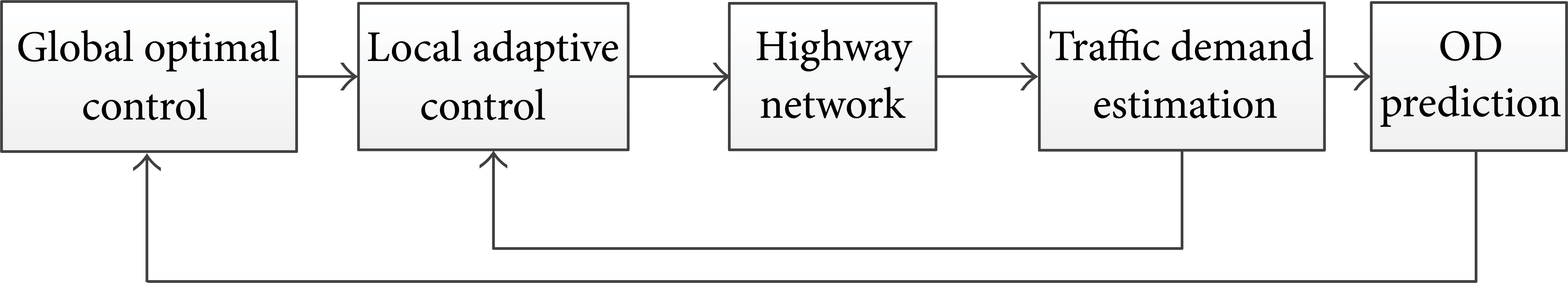
System structure of the hierarchical optimal control system.

2.2. Model of the Traffic Flow in Freeway

Traffic flow model is the mathematical framework which describes the relations between the speed, the density, and the flow [14]. Looking from viewpoint of system optimization and in order to guide and control traffic flow, each kind of shapes and the rules of the traffic flow will be studied. Fast, stable, and highly effective traffic flow model will be established. The main study for traffic flow model is as follows: according to traffic flow situation and corresponding theories, the traffic flow model will be built and the simulation research will be done [14]. This paper will build the traffic flow model based on highway macroscopic transportation: MACRO model [15]. MACRO model will be introduced as the following contents:

$\begin{array}{c}\rho \left(i,k+\mathrm{1}\right)=\rho \left(i,k\right)+\frac{T}{l_i·n_i}\left[q\left(i-\mathrm{1},k\right)-q\left(i,k\right)+r\left(i,k\right)-e\left(i,k\right)\right]\\ q\left(i,k\right)=\rho \left(i,k\right)·v\left(i,k\right)·n_i\\ v\left[\rho \left(i,k\right)\right]=v_f{\left[\mathrm{1}-{\left(\frac{\rho \left(i,k\right)}{{\rho }_{\text{jam}}}\right)}^{\alpha }\right]}^{\beta }.\end{array}$

(1)

At the entrance and the exit, namely, i = 1 and i = N:

$\begin{array}{c}\rho \left(\mathrm{1},k+\mathrm{1}\right)=\rho \left(\mathrm{1},k\right),v\left(\mathrm{1},k+\mathrm{1}\right)=v\left[\rho \left(\mathrm{1},k\right)\right]\\ \rho \left(N,k+\mathrm{1}\right)=\rho \left(N,k\right),v\left(N,k+\mathrm{1}\right)=v\left[\rho \left(N,k\right)\right].\end{array}$

(2)

When metering on-ramp, change of the queuing length must be studied, so there obviously is

$p\left(i,k+\mathrm{1}\right)=p\left(i,k\right)+T\left[d\left(i,k\right)-r\left(i,k\right)\right].$

(3)

Besides the above state equation, r(i,k) must follow the upper limit and the lower limit constraints:

$r_{i\min }\le r\left(i,k\right)\le r_{i\max },$

(4)

where i represents the serial number of sections, i = 1,…,N; ρ(i,k) represents the average density of vehicles on section i at time k (veh/km/lane); l _i is the segment length; n _i represents the number of lanes on section i; r(i,k) represents the traffic flow on entrance ramp of section i at time k; e(i,k) represents the exit ramp traffic flow on section i at time k; v(i,k) represents the interval speed of vehicles on section i at time k (km/h); p(i,k) represents the queuing length of vehicles on entrance ramp of section i at time k; T represents the sampling period; d(i,k) is the demand on segment i at the time k; v _f is the free flow speed; ρ_jam is the lowest density of the jam; α, β are two model parameters; q(i,k) is the number of the vehicles on segment i at the time k (veh/h/lane). ρ(i,k), v(i,k), and p(i,k) are state variables, r(i,k) and e(i,k) are control variables, and q(i,k) is the output variable.

Except to model the traffic flow, according to the above state equations of the traffic flow model and the constraints, this paper establishes the control objectives and the constraints for global optimal control module (for details, see Section 2.4).

2.3. Traffic Demand Estimation and OD Prediction

Traffic demand estimation module will be used to estimate real-time traffic demand, OD prediction module will be used to predict the total transportation demands in a long time, and boundary of the queue length will be determined ahead of time. In this paper, we used estimation module to estimate the real-time traffic conditions for local adaptive control module, and the OD prediction module predicts the total traffic demands in a long time and determines the upper bound of the future queuing length in advance, so that we can realize “premanagement” for dynamic traffic management.

When carrying on the real-time OD matrix estimation and prediction in this paper, the state space model of Ashok [16] will be used. The state variable is defined as a deviation: δx _h = x _h − x _h ^H ; here x _h are vectors of all OD flows and the corresponding historical estimates have been given as x _h ^H . This deviation follows an autoregressive process:

$\delta {\mathbf{x}}_{h+\mathrm{1}}={{\displaystyle \sum }}_{p=h+\mathrm{1}-q^{\prime }}^h{f}_{h+\mathrm{1}}^p\delta {\mathbf{x}}_p+{\mathbf{w}}_{h+\mathrm{1}}.$

(5)

Here, f_{h + 1} ^p is an autoregressive coefficient matrix reflecting the effects of δx _p on δx_{h + 1}; q′ is the order of the autoregressive process; w_{h + 1} is the random error, whose content E(w_{h + 1}) = 0; and E(w _h w _l ^T ) = Q _h δ _hl , Q _h is the error covariance matrix, ${\delta }_{hl}=\{\begin{array}{cc}\mathrm{1},& h=l\\ \mathrm{0},& h\ne l\end{array}$

$\mathit{\delta }{\mathbf{y}}_h={{\displaystyle \sum }}_{p=h-p^{\prime }}^h{\mathbf{a}}_h^p\mathit{\delta }{\mathbf{x}}_p+{\mathbf{v}}_h,$

(6)

where δy _h = y _h − y _h ^H = y _h − ∑_{p = h − p′} ^h a _h ^p x _p ^H , y _h is the transportation volume measured during interval h, and y _h ^H is the corresponding historical value [17]. The matrix a _h ^p is an assignment matrix of contributions of δx _p to δy _h , and it is the fraction of the rth OD that departed its origin during interval p and crossed the counting point during interval h; (p′ + 1) is the maximum number of time intervals taken to travel between OD pairs of the network. v _h is the measurement error, and E(v _h ) = 0.

Equations (5) and (6) construct the state space model for dynamic OD estimation and prediction. Kalman filter is used to estimate and predict OD information.

2.4. Global Optimal Control

If we do not consider the lane changing of vehicles, the global optimal control module can take into account many on-ramps on sections of the freeway and determine the metering rate of the on-ramp based on the estimated information of traffic demands to optimize the overall performance indicator [12]. This control scheme is implemented as follows.

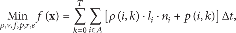
2.4.1. Performance Indicators

The running time of minimized vehicles in the freeway and the waiting time on the on-ramp are taken as the performance indicators.

1. In the time period [0,T], the total running time of vehicles on mainline of the freeway is given by

   $T_{\mathrm{1}}={{\displaystyle \int }}_{\mathrm{0}}^T{{\displaystyle \sum }}_{i\in A}\left[\rho \left(i,t\right)·l_i·n_i\right]dt,$

   (7)

2. where A is the set of serial numbers of freeway sections.

3. The waiting time of vehicles on the entrance ramp is given by:

   $T_{\mathrm{2}}={{\displaystyle \int }}_o^T{{\displaystyle \sum }}_{i\in A}p\left(i,t\right)dt.$

   (8)

Then, the total running time of vehicles is given by

$T=T_{\mathrm{1}}+T_{\mathrm{2}}={{\displaystyle \int }}_{\mathrm{0}}^T{{\displaystyle \sum }}_{i\in A}\left[\rho \left(i,t\right)·l_i·n_i+p\left(i,t\right)\right]dt.$

(9)

After discretization, the above equation can be rewritten as

$Z={{\displaystyle \sum }}_{k=\mathrm{0}}^T{{\displaystyle \sum }}_{i\in A}\left[\rho \left(i,k\right)·l_i·n_i+p\left(i,k\right)\right]\Delta t.$

(10)

Then, the objective function is given by

$\underset{\rho ,v,f,p,r,e}{\mathrm{Min}}f\left(\mathbf{x}\right)={{\displaystyle \sum }}_{k=\mathrm{0}}^T{{\displaystyle \sum }}_{i\in A}\left[\rho \left(i,k\right)·l_i·n_i+p\left(i,k\right)\right]\Delta t,$

(11)

where x = {ρ(i,k),v(i,k),f(i,k),p(i,k),r(i,t),e(i,k)} represents the set of variables.

2.4.2. Constraints

The upper and lower limit constraints which must be followed by the control rate of on-ramp are

$r_{i\min }\le r\left(i,k\right)\le r_{i\max }.$

(12)

Meanwhile, the queuing length of on-ramp i cannot exceed its queuing capacity p _imax ; namely,

$p\left(i,k\right)+T\left[d\left(i,k\right)-r\left(i,k\right)\right]\le p_{i\max }.$

(13)

Obviously, the queuing length p(i,k + 1) ≥ 0; namely,

$\begin{array}{c}p\left(i,k\right)+T\left[d\left(i,k\right)-r\left(i,k\right)\right]\ge \mathrm{0}\\ \rho \left(i,k\right)\le {\rho }_{\text{jam}}.\end{array}$

(14)

Furthermore, all variables meet the nonnegative constraints, namely, ρ(i,k) > 0, v(i,k) > 0, f(i,k) > 0, p(i,k) > 0, r(i,k) > 0, and e(i,k) > 0.

2.4.3. Solution Algorithm

The above mentioned global optimal control problem can be solved as a nonlinear programming problem with constraints. The general description of nonlinear programming is as follows:

$\begin{array}{c}\begin{array}{cc}\underset{x\in R^n}{\min }& f\left(\mathbf{x}\right)\hfill \\ \text{s}.\text{t}.& g_i\left(\mathbf{x}\right)=\mathrm{0},\hspace{1em}i=\mathrm{1,2},\dots ,m_e\\ & \hspace{1em}{h}_i\left(\mathbf{x}\right)\le \mathrm{0},\hspace{1em}i=m_e+\mathrm{1},\dots ,m\\ & {\mathbf{x}}_l\le \mathbf{x}\le {\mathbf{x}}_u,\hspace{0.17em}\hspace{1em}\hspace{1em}\hspace{1em}\hspace{1em}\end{array}\end{array}$

(15)

where x represents the optimized variable; f(x) represents the objective function; g _i (x) and h _i (x) return the estimated values at x of equality and inequality constraints. The sequential quadratic programming (SQP) [18] has good superlinear convergence property and holds a very important status in nonlinear programming. From the point of view of the effect of actual values, SQP algorithm is very effective for optimization problems with non-linear constraints. So, SQP was used to solve the global optimal control problem after transforming it into the standard form of a nonlinear problem. The specific implementation procedures are as follows.

Step 1. Give the initial point of any variable: x = {ρ(i,0),v(i,0),f(i,0),p(i,0),r(i,0),e(i,0)} and the initial value of Hessian matrix B₁ (symmetric positive definite matrix or semisymmetric positive definite matrix) needed when solving the quadratic programming subproblem.

Step 2. Form and solve the quadratic programming subproblem: J = min⁡[(1/2)d _T B _k d + ∇f( x _k ) ^T d], and meet the constraint condition: g _k + A _k ^T d = 0, where

$\begin{array}{c}{\mathbf{g}}_k={\left(g_{\mathrm{1}}\left({\mathbf{x}}_k\right),g_{\mathrm{2}}\left({\mathbf{x}}_k\right),\dots ,g_m\left({\mathbf{x}}_k\right)\right)}^T\\ {\mathbf{A}}_k=\left(\nabla g_{\mathrm{1}}\left({\mathbf{x}}_k\right),\nabla g_{\mathrm{2}}\left({\mathbf{x}}_k\right),\dots ,\nabla g_m\left({\mathbf{x}}_k\right)\right).\end{array}$

(16)

Step 3. Record the calculated optimal solution d _k which is the direction of search. If ∥d _k ∥ ≤ ε, then x_* = x _k will be the optimal solution; stop the calculation. Otherwise, go to Step 4, where ε represents the allowable error.

Step 4. Solve the minimum point of Fletcher penalty function by the iterative algorithm:

$\varphi \left(\mathbf{x},\sigma \right)=f\left(\mathbf{x}\right)-{\lambda }^T\left(\mathbf{x}\right)g\left(\mathbf{x}\right)+\frac{\mathrm{1}}{\mathrm{2}}\sigma {\parallel g\left(\mathbf{x}\right)\parallel }^{\mathrm{2}}.$

(17)

This minimum value is the step size in the search, where σ represents the penalty factor.

Step 5. Calculate x_{k + 1} = x _k + β _ki d _k , where β _ki represents the test step of the iterative algorithm when solving the minimum value of the penalty function. Its initial value is 1.

Step 6. Iteratively update the Hessian matrix to maintain its positive definite (or semipositive definite) property,

$B_{k+\mathrm{1}}=B_k+\frac{{\mathbf{q}}_k{\mathbf{q}}_k^T}{{\mathbf{s}}_k^T{\mathbf{s}}_k}-\frac{B_k{\mathbf{s}}_k{\mathbf{s}}_k^T{B}_k}{{\mathbf{s}}_k^T{B}_k{\mathbf{s}}_k},$

(18)

where

$\begin{array}{c}{\mathbf{q}}_k=\nabla f\left({\mathbf{x}}_{k+\mathrm{1}}\right)-\nabla f\left({\mathbf{x}}_k\right)\\ {\mathbf{s}}_k={\mathbf{x}}_{k+\mathrm{1}}-{\mathbf{x}}_k.\end{array}$

(19)

Return to Step 2.

2.5. Local Adaptive Control

The adaptive control is a very important aspect in the automatic control theory. Since the 1970s, researchers began to apply it to the field of traffic control. Linear quadratic optimal control has been widely used ever since [18].

The dynamic process of traffic system can be briefly expressed as

$x_{t+\mathrm{1}}=f\left(x_t,u_t\right),$

(20)

where x _t and u _t represent the stable variable and control variable, respectively. Payne made an assumption that if the changes of traffic system are always controlled in the range of nominal conditions [19], the linear equation (15) can be written as

$x_{t+\mathrm{1}}=A{x}_t+B{u}_t,$

(21)

where A, B are constant matrices.

The objective of adaptive control is to minimize the difference between the minimum state variable, control variable, and their nominal state variable $(\stackrel{-}{x},\stackrel{-}{u})$ , that is, minimizing the quadratic performance function:

$J={{\displaystyle \sum }}_t\left\{{\parallel x_t-\stackrel{-}{x}\parallel }^{\mathrm{2}}+\omega {\parallel u_t-\stackrel{-}{u}\parallel }^{\mathrm{2}}\right\}.$

(22)

For the linear traffic system described in (15), the following adaptive control can be obtained through minimizing this quadratic performance index:

$u_t=\stackrel{-}{u}-L\left(\stackrel{-}{x},\stackrel{-}{u}\right)\left(x-\stackrel{-}{x}\right),$

(23)

where $L(\stackrel{-}{x},\stackrel{-}{u})$ represents the control gain matrix, which can be calculated by the Riccati equation [20]: $\dot{L}\left(t\right)=-L\left(t\right)A\left(t\right)-{\mathbf{A}}^T\left(t\right)L\left(t\right)+L\left(t\right)B\left(t\right)R^{-\mathrm{1}}\left(t\right)B^T\left(t\right)L\left(t\right)-Q\left(t\right)$ , where Q, R represent any positive definite symmetric matrix.

In this hierarchical optimal control system, the local adaptive control on section i is the density deviation determined according to the current density ρ(i,k) on the ramp and the density $\stackrel{-}{\rho }(i,k)$ obtained through optimizing the global optimal control layer. The metering rate of the on-ramp is regulated to make it close to the optimal metering rate $\stackrel{-}{r}(i,k)$ obtained through optimizing the global optimal control layer:

$r\left(i,k\right)=\stackrel{-}{r}\left(i,k\right)-L·\left(\rho \left(i,k\right)-\stackrel{-}{\rho }\left(i,k\right)\right).$

(24)

If only using the local adaptive control, the metering rate of on-ramp shall be determined by its a priori value; the capacity is the expected capacity and a constant. The linear quadratic adaptive control expression is as follows:

$r\left(i,k\right)=r\left(i,k-\mathrm{1}\right)-K·\left(\rho \left(i,k\right)-{\rho }_d\left(i,k\right)\right).$

(25)

Here K is a constant control gain matrix, ρ _d (i,k) is a constant desired density, in this paper, ρ _d (i,k) = 55 veh/km/lane, and r(i,k − 1) is the on-ramp metering rate at k − 1.

3. Simulation Research

The freeway network as shown in Figure 2 was studied in this paper. The numbers on the signal are sections in the networks. There are 9 sections in the transverse direction, and all of them are one-way four-lane roads. The longitudinal direction is the on-ramp and off-ramps, and all of them only have one lane. The length of each section is 3 km. The one-step predicted values of traffic demands on the mainline and various ramp entrances are shown in Figure 3. There are 19 OD pairs and 1 mainline and 4 on-ramps (number 11 ramp, number 13 ramp, number 15 ramp, and number 17 ramp).

Figure 2:

Traffic networks.

Figure 3:

Traffic demands of various OD pairs.

The model used in the traffic flow modeling and simulation was MACRO model [15]. It is assumed that the initial values of metering rates of various ramps are all 600 veh/h, the initial values of traffic flows at the off-ramp are all 400 veh/h/lane, the maximum metering rate is r_max = 900 veh/h, the minimum metering rate is r _min = 180 veh/h, the free flow speed is v _f = 100 km/h, and the congestion density is ρ_jam = 130 veh/km/lane. In the speed-density model, the model parameters α, β were obtained by parameter calibration using data mining techniques introduced in [14]. In this example, α = 1.7, β = 2, the simulation time is 1 hour, the cycle length is T = 3 min, the changing of lanes is not considered, and the initial densities of various sections are 18.37, 25.0, 23.8, 0, 30.0, 31.0, 0, 42.0, and 20.0 veh/km/lane, respectively. Traffic congestion occurs on the mainline from t = 12 min to t = 30 min, and the maximum density reaches up to 120 veh/mile/lane which is close to the congestion density. The traffic congestion phenomenon spreads from section 4 to section 8, which occupies more than half of the mainline of the entire freeway network. The distribution of traffic density in the road network is shown in Figure 4(a).

Figure 4:

Three-dimensional density changes of various sections in different control schemes.

To fully illustrate the control effect of hierarchical optimal control, only the control effects of the local adaptive control module and global optimal control module are compared with those of the model proposed in this paper when the simulation parameters and initial conditions are completely the same.

Figure 4(b) shows the changing of traffic density in the road network when adopting the local adaptive control; Figure 4(c) shows the densities profiled by only using global optimal control; Figure 4(d) shows the changing of traffic density in the freeway network when adopting the hierarchical optimal control. It can be seen through comparing Figure 4 that the implementation of any control scheme can ease the traffic congestion in the freeway network. But the control effect of the hierarchical optimal control is better than that of the others. The former can better ease the traffic congestion.

The total running time of vehicles (the vehicle travel times of five main OD pairs) is provided in this paper, as listed in Table 1. With any of the control algorithms, the mainline travel time reduces to less than 190 seconds. However, the travel times for the ramps are mixed. Some of them increase and others decrease. Since mainline carries the largest traffic demand, a small reduction in its travel time contributes to a large improvement in the system performance. With global optimal control, the travel times drop significantly. However, travel times on ramp 2, ramp 3, and ramp 4 increase. As shown in the density profiles in Figure 4(a), ramp 13 is the bottleneck of the network. In order to reduce the congestion in this bottleneck, the control algorithm will cost much more time to meter traffic flow that will cause a delay on ramp 13. The adoption of both the local adaptive control and the hierarchical optimal control can save a lot of travel time for travelers, but the control effect of the latter is better than that of the former, and the latter can save more travel time.

Table 1:

Travel times in different control schemes.

	Control method	OD pairs
		Mainline (1–10)	Ramp 1 (11–10)	Ramp 2 (13–10)	Ramp 3 (15–10)	Ramp 4 (17–10)
Travel time(s)	No control	379	325	346	260	314
	Local adaptive control	199	182	259	130	169
	Global optimalcontrol	193	319	586	410	354
	Hierarchical control	197	246	324	147	286
Saved time(s)	Local adaptive control	180	143	87	130	145
	Global optimal control	186	6	−240	−150	−40
	Hierarchical control	182	79	22	113	28

4. Conclusions

By following the design principles of breaking down and coordination of a large system, an optimal control system of the dynamic traffic flow on a freeway was established. The control system is divided into four modules according to the hierarchical concept: the OD prediction module predicts the total traffic demands in a long time and determines the upper bound of the future queuing length in advance; the global optimal control module predicts the future traffic state and establishes the coordination constraints for each ramp in the network; the traffic demand estimation module estimates the real-time traffic conditions for each ramp; the local adaptive control module regulates ramp metering rate according to the estimated information of the real-time traffic conditions and the results optimized by the global optimal control module. They coordinate the benefits of various on-ramps and realize the dynamic traffic management of freeway from the “passive response type” to the “active preventative type.” The simulation results show that this system has a significant effect in easing the traffic congestion and saving the travel time of vehicles and also plays an important role in the optimization of the overall performance of the freeway network.

Conflict of Interests

The authors declare that there is no conflict of interests regarding the publication of this paper.