Sage Journals: Discover world-class research

Abstract

Wireless sensor networks (WSNs) are receiving a lot of research attention due to continual improvement in the technologies used by these networks. The energy efficiency of sensor nodes and the network as a whole is of specific importance. One possible area where energy savings can be made lies within the routing protocols employed; however, these protocols are typically only simulated. In this work we develop a WSN testbed and conduct investigations on the fidelity of simulated energy-aware WNS routing protocols. It was found that the real-world performance of these energy-aware protocols was significantly lower than that predicted by simulation models. This can be mainly attributed to chip-level effects not taken into account by simulation models, leading to simulated results that cannot be achieved in real-world deployments. This work illuminates the shortfalls of existing simulation models and suggests ways in which these models can be improved. Additionally the testbed allows other energy-aware routing protocols to be investigated easily.

1. Introduction

In recent years wireless sensor networks (WSNs) have become more popular due to their wide range of application areas and a decrease in the cost, size, and power consumption of sensor nodes (SNs) [1]. The majority of existing SNs are powered by constrained energy sources which include batteries and power scavenging devices [1]. Due to the limited energy available to the sensor network all aspects of the network must be optimised in order to minimise the energy consumption. The routing solution employed in a WSN affects the energy consumption of the network, and thus WSN routing protocols are an active area of research [2–5]. In order to compare existing routing protocols and to develop improved protocols, the energy consumption characteristics of these protocols must be investigated [2, 3].

The majority of studies on the energy efficiency of WSN routing protocols are conducted using simulations [4–6]. This is because simulations offer a more time and cost effective solution when compared to experimentation. Some common axioms used when modelling wireless networks are described by Kotz et al. in [7]. Most simulations do not take all the factors that influence a WSN into account, and factors that are taken into account are not always 100% accurate. This is especially true in the case of the energy consumption characteristics of the transceiver modules of the SNs.

In this work a WSN testbed is developed that allows the characterisation of the energy consumption of a SN, both from transceiver and routing protocol points of view. Insight is provided into how the energy consumption of realistic SNs differs from simulated works by implementing a MTTPR routing scheme on the testbed. Additionally recommendation as to how simulation models could be improved is also provided.

In the remainder of this paper some background to wireless sensor networks, IEEE 802.15.4, and sensor nodes is provided in Section 2. Section 3 details the development of a custom SN, which is used for the testbed configured in Section 4. Section 5 provides details on the experimental setup, with the results and discussion presented in Sections 6 and 7. Concluding remarks are provided in Section 8.

2. Background

This section provides some background on WSNs, the IEEE 802.15.4 standard, and energy-aware routing schemes.

2.1. Wireless Sensor Network

A WSN is a group of spatially removed SNs which form a cooperative wireless network. Not all of the SNs in such a network can communicate with each other directly. These nodes forward data to nodes that are outside their communication range in a multihop fashion using other SNs. Some nodes in a WSN act as network gateways. These nodes are called sink nodes. A WSN can consist of hundreds and even thousands of nodes. Figure 1 depicts a typical WSN. In recent years commercial interest in WSNs has moved into the direction of large static networks which is taken into account by the Internet Engineering Task Force (IETF) Routing over Low-Power and Lossy Networks (ROLL) standard [8]. Some promising WSN application areas include [9, 10]

(i)

home and automation;

(ii)

personal health care;

(iii)

industrial control;

(iv)

utility meter communication;

(v)

automatic meter reading and demand-side management;

(vi)

battlefield surveillance.

Figure 1

Depiction of a typical wireless sensor network (WSN).

2.2. IEEE Standard 802.15.4

The IEEE 802.15.4 standard defines a physical communication layer and a data link layer for low-rate wireless personal area networks (LR-WPANs). The standard gives attention to energy conservation in such wireless networks [11]. The Medium Access Control (MAC) and physical layer (PHY) specifications of the standard can be found in IEEE Std. 802.15.4-2003 [12]. The standard utilises carrier sense multiple access with collision avoidance (CSMA-CA) and supports point-to-point and star network topologies. Table 1 depicts the frequency band, modulation, and data rate details of the IEEE 802.15.4 standard physical layer [12]. The IEEE 802.15.4 standard defines four frame structures which were designed to reduce complexity while still providing a robust solution for noisy channels. These frames include

(i)

a beacon frame;

(ii)

a data frame;

(iii)

an acknowledgement frame;

(iv)

a MAC command frame.

Table 1

IEEE 802.15.4 physical layer implementations.

PHY (MHz)	Frequency band (MHz)	Modulation	Bit rate (kb/s)
868 (default)	868–868.6	BPSK	20
915 (default)	902–928	BPSK	40
868 (optional)	868–868.6	ASK	250
915 (optional)	902–928	ASK	250
868 (optional)	868–868.6	O-QPSK	100
915 (optional)	902–928	O-QPSK	250
2450	2400–2483.5	O-QPSK	250

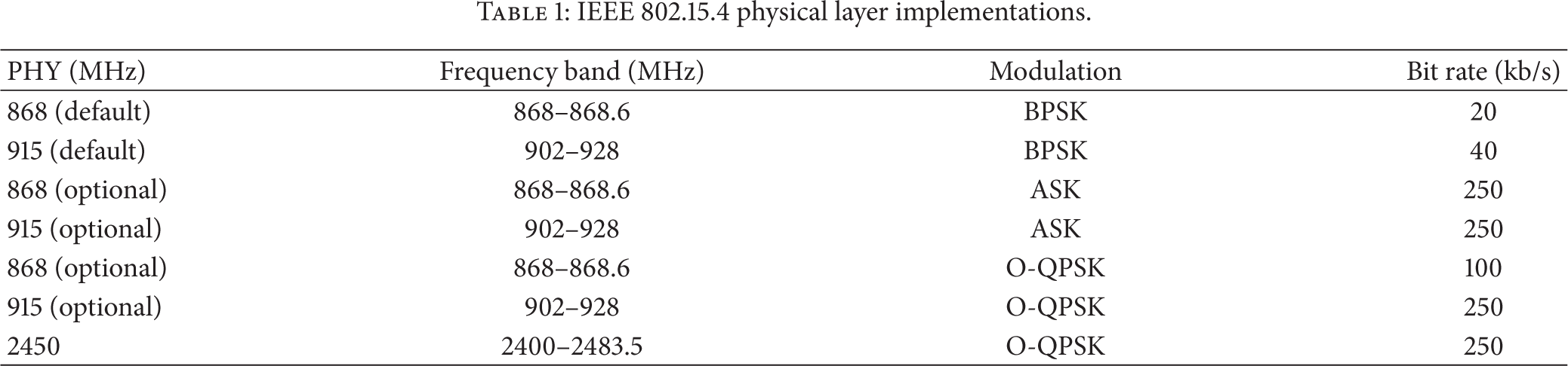
The data and acknowledgement frames are used to accomplish data transfer between nodes. Beaconing serves as a synchronization service within the network, and the MAC command frame is used for network management and control [11].

2.3. Energy-Aware Routing Schemes

This section details some common energy-aware routing schemes.

(1) Minimum total transmission power routing: minimum total transmission power (MTTP) routing selects the path between communicating nodes based on the minimum transmission power. When forwarding data between nodes the route with the minimum total transmission power is selected. Although MTTPR is an improvement over simplistic routing schemes, such as shortest path first routing, it does not take an individual node's remaining energy into account. This could lead to certain nodes being overused.

Mathematically, the total transmission power $P_{j}$ for route j can be calculated by means of (1). In (1) D represents the total distance (in hops) between the source ( $n_{0}$ ) and the destination ( $n_{D}$ ) nodes. $P (n_{i}, n_{i + 1})$ represents the transmission power between nodes $n_{i}$ and $n_{i + 1}$ [13]:

\begin{matrix} P_{j} = \sum_{i = 0}^{D - 1} ‍ P (n_{i}, n_{i + 1}) . \end{matrix}

(1)

All possible routes form a set A from which the MTTP route (m) is selected by means of

\begin{matrix} P_{m} = \min_{j \in A} P_{j} . \end{matrix}

(2)

(2) Minimal-battery cost routing: the minimal-battery cost (MBC) routing scheme selects the highest remaining total battery life path between communicating nodes [14]. As is the case with MTTP routing, MBCR does not take an individual node's energy capacity into account. As such, individual nodes may be subjected to overuse.

The remaining battery capacity of node $n_{i}$ , ranging from 0 to 100, is represented by $b_{i}$ . The willingness of a node to forward data, based on its remaining battery capacity, is denoted by $f_{i}$ in

\begin{matrix} f_{i} (b_{i}) = \frac{1}{b_{i}} . \end{matrix}

(3)

The total battery cost for route k, $B_{k}$ , is calculated by means of (4). As with MPPT routing the distance between the source and destination nodes (in hops) is denoted by D:

\begin{matrix} B_{k} = \sum_{i = 0}^{D - 1} ‍ f_{i} (b_{i}) . \end{matrix}

(4)

All possible routes form a set A, from which the minimal battery cost route, z, can be calculated as per

\begin{matrix} B_{z} = \min_{k \in A} B_{k} . \end{matrix}

(5)

In the event that two or more routes have the same battery cost the shortest route is selected.

(3) Min-max battery cost routing: min-max battery cost (MMBC) routing attempts to improve MBCR by avoiding the nodes with the least amount of energy remaining. This ensures that no single node within the network gets overused. However, there is no guarantee that the chosen route is a MTTP route or a minimal battery cost route. Equation (6) redefines the cost of route k for the MMBCR scheme:

\begin{matrix} B_{k} = \max_{i \in k} f_{i} (b_{i}) . \end{matrix}

(6)

The min-max battery cost route (s) is calculated from (7). As before A is a set which contains all of the possible routes [13]. Also, as was the case with MBCR, where two, or more, routes have a similar cost metric, the shortest route is selected:

\begin{matrix} B_{s} = \min_{k \in A} B_{k} . \end{matrix}

(7)

(4) Conditional Max-Min Battery Capacity Routing: Conditional Max-Min Battery Capacity (CMMBC) routing is a combination of MTTPR and MMBCR. The MTTPR scheme is used to choose routes; however, if the remaining energy of a node on the chosen route is below a certain threshold, γ, another route is chosen. This ensures that single nodes do not get overused [13].

(5) Minimum total transceiving power: the minimum total transceiving power (MTTCP) routing scheme is an extension of the MTTP routing scheme. The MTTCP routing scheme attempts to minimize the total transmission and reception power used on the path between communicating nodes [15]. Similarly to the MPPT scheme no guarantee is provided that individual nodes will not be overused.

(6) Minimum total reliable transmission power: the minimum total reliable transmission power (MTRTP) routing scheme is yet another extension of the MTTP routing scheme. The MTRTP routing scheme takes the reliability and the transmission power setting of each link into account [15].

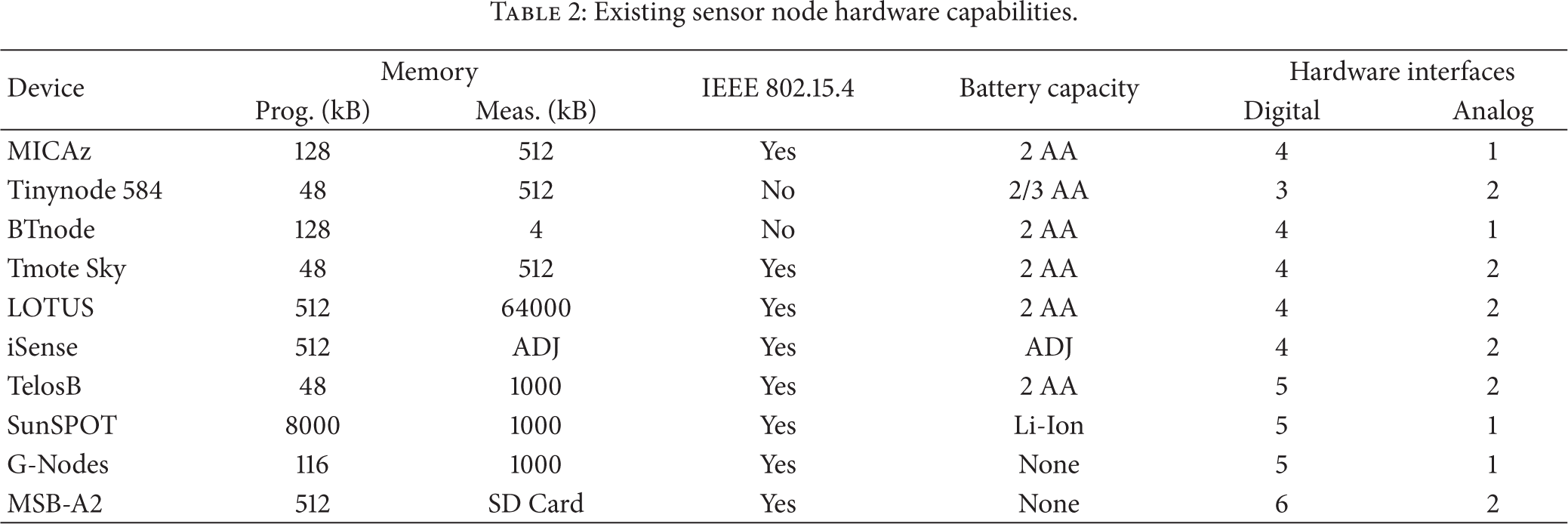
2.4. Existing Sensor Nodes

From surveys conducted by Hellbruck et al. [16] and Steyn and Hancke [17] in 2011, SNs commonly used in WSN testbeds include MICAz, SunSPOT, iSense, TelosB, G-Node, and Tmote Sky. Table 2 provides some features of existing SNs [18–27]. A brief perusal of the information contained in Table 2 shows that microcontrollers deployed in SNs range from low-power 8-bit devices to more powerful 32-bit devices. When selecting a SN microcontroller the energy efficiency and the computational power requirements of the SN must be kept in mind in order to maximize the SN lifetime. This is especially true for SNs powered by limited energy sources. In terms of communication hardware the majority of SN designs make use of IEEE standard 802.15.4 compliant transceivers. Most of the SNs are powered by two AA (R6) batteries, which are typically disposable as SNs will not typically be redeployed during their lifetime [28]. None of the existing nodes feature integrated battery charging capabilities. Whilst this is not critical to the operation of a WSN SN it hampers the ease of use in a testbed deployment. The WASPMOTE [29] features a modular design with many available sensor and transceiver options and features integrated battery charging but cannot measure its own energy consumption. For this reason, a SN capable of measuring its own energy consumption is developed. The SN is developed with a specific focus on testbed deployment.

Table 2

Existing sensor node hardware capabilities.

Device	Memory		IEEE 802.15.4	Battery capacity	Hardware interfaces
Device	Prog. (kB)	Meas. (kB)	IEEE 802.15.4	Battery capacity	Digital	Analog
MICAz	128	512	Yes	2 AA	4	1
Tinynode 584	48	512	No	2/3 AA	3	2
BTnode	128	4	No	2 AA	4	1
Tmote Sky	48	512	Yes	2 AA	4	2
LOTUS	512	64000	Yes	2 AA	4	2
iSense	512	ADJ	Yes	ADJ	4	2
TelosB	48	1000	Yes	2 AA	5	2
SunSPOT	8000	1000	Yes	Li-Ion	5	1
G-Nodes	116	1000	Yes	None	5	1
MSB-A2	512	SD Card	Yes	None	6	2

3. Sensor Node Design

The requirements of a SN suitable for testbed deployment were first outlined by Krige et al. in [30] and are summarized as follows:

(i)

capable of measuring SN's own energy consumption;

(ii)

integrated battery recharging;

(iii)

ease of protocol implementation;

(iv)

modular design that is standards compliant.

A product development methodology, based on the systems engineering process, was followed. Hence, the operational environment in which the testbed was to operate was studied in order to derive the operational requirements. By taking all requirements into account the operational architecture in Figure 2 was developed. By making use of the operational architecture the functional architecture of the sensor node was developed. In Figure 3 the functional architecture of the SN can be seen. Notice that the SN is of modular design with a main board, sensor module, and transceiver module. This is similar to the architecture of the WASPMOTE but with the addition of energy measuring hardware. Each SN is capable of measuring and recording its own energy consumption and remaining battery capacity. Sensor modules and transceiver modules are easily replaced and this increases the flexibility of the SN in testbed deployments. The addition of an integrated lithium-ion battery and charging circuitry improves the usability of the SNs.

Figure 2

Operational architecture of WSN testbed.

Figure 3

Functional architecture diagram of WSN sensor node.

Each of the main components of the SN will now be discussed.

3.1. Microcontroller

The microcontroller is responsible for controlling the SN as well as implementing the communications protocol. As such, it must provide sufficient resources whilst at the same time being as energy efficient as possible. A 16-bit processor from Microchip (PIC24FJ128GA310) was selected as this provided more adequate resources whilst at the same time being energy efficient. The microcontroller is part of Microchip's nanoWatt Extreme Low-Power (XLP) technology family of devices and consumes only 20.7 mW and a maximum idle mode power consumption of 4.2 mW when operating at 16 MIPS [31]. Sleep mode power consumption can be as low as $12.54 μ$ W at room temperature. The microcontroller also features an integrated real-time clock and calendar (RTCC) which is supplied with an independent 3 V battery power source and a high accuracy 32.768 kHz crystal. The integrated RTCC features a resolution of 1 second with an error of less than 3 seconds per month [32].

3.2. Energy Measurement Unit

To implement the energy measurement unit a current sense resistor and a voltage divider circuit were used. A 300 m $Ω 1$ % shunt resistor was connected to an analog front end from Microchip (MCP3911) and provides a measurement resolution of 40 nA. A voltage divider circuit with $1 %$ tolerance resistors is used to measure the supply voltage (via the analog front end) to a resolution of 582 nV [33].

3.3. Communications Interface

By using the MRF24J40MC IEEE standard 802.15.4 compliant RF transceiver from Microchip the SN design is simplified. Firstly, the RF transceiver is standards compliant, and secondly the MiMAC protocol stack can be freely used. The Microchip Wireless (MiWi) Media Access Controller (MiMAC) defines a MAC and PHY layer which is supported across all Microchip transceivers. Standards compliance is achieved by the combination of the MiMAC stack and a suitable transceiver. Additionally the use of the MiMAC simplifies the implementation of various routing protocols [34], and it is thus of great value in testbed applications.

3.4. Form Factor and Interconnects

The overall design of the SN is modular, as the communications module and the sensor module can be easily replaced, depending on the experimental requirements. In Figure 4, the communications module, measurement and control module, and the sensor module can clearly be seen. Also the DE9 connector at the bottom edge of the measurement and control module that allows (a) the programming of the module by in-circuit means and (b) charging of the integrated battery are of interest. Four status LEDs are available to the user to inform the user of the current state of the SN (either during charging or other experimental processes). A single connector forms one convenient interface for node charging, node programming, and serial communication.

Figure 4

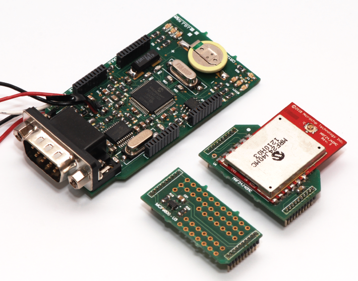
Photograph of a sensor node with its sensor and transceiver modules being removed.

3.5. Power Consumption

Typical node power consumption (calculated from device datasheet information) is outlined in Table 3. A 1100 mAh lithium-ion battery powers the SN during experimental deployment and depending on transmission power settings should provide at least 10 hours of operational life. The battery status is displayed via three (3) LEDs and the battery can be charged by the integrated circuitry via the DE9 connector.

Table 3

Sensor node power consumption (calculated).

Component	Typical current consumption (mA)
RF transceiver (MRF24J40MC @ 19 dBm)	120
Microcontroller (PIC24FJ128GA310)	4.9
Analog front-end (MCP3911 BOOST = 10_b)	2.5
Miscellaneous components	1

Total power consumption	128.4

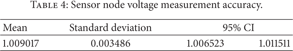
3.6. Measurement Accuracy

The accuracy of the SNs’ energy measurement circuitry was determined by comparing the SNs’ measurements with those of a calibrated precision bench-top multimeter (Tektronix DMM4050). Current measurement accuracy was compared for the following three scenarios:

(i)

SN is idle;

(ii)

SN is transmitting at $- 26.4$ dBm (minimum);

(iii)

SN is transmitting at 19 dBm (maximum).

In each case the accuracy of the SN measurement is denoted by the ratio of the SN measurement with the bench-top (BM) measurement, to wit $V_{SN} / V_{BM}$ . In the case of voltage measurement the SN mode is of no concern and, as such, average values were used. A summary of the descriptive statistics (mean, standard deviation, and 95th% confidence intervals) is provided in Tables 4 and 5.

Table 4

Sensor node voltage measurement accuracy.

Mean	Standard deviation	95% CI
1.009017	0.003486	1.006523	1.011511

Table 5

Sensor node current measurement accuracy.

Sensor node state	Mean	Standard deviation	95% CI
Idle	1.033666	0.008019	1.027502	1.039830
Minimum TX power	1.017322	0.010565	1.009764	1.024880
Maximum TX power	1.027214	0.016341	1.015524	1.038904

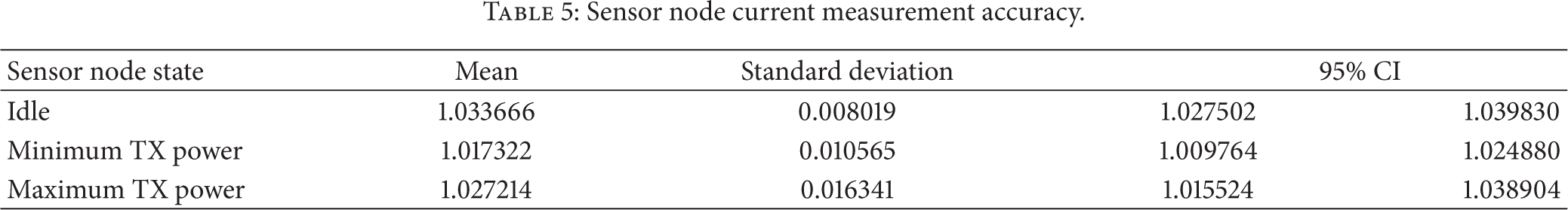
From the values in Tables 4 and 5 it is clear that the SN's measurements are slightly higher than those obtained from the bench-top multimeter. This, however, is not an issue as the measurements are well within acceptable ranges. Each SN could be individually calibrated to provide exact measurements, but this complicates testbed deployment. As such a small variance (as was observed) in SN measurements is acceptable. A completed SN is shown in Figure 5.

Figure 5

Photograph of a completed sensor node.

4. Testbed Setup

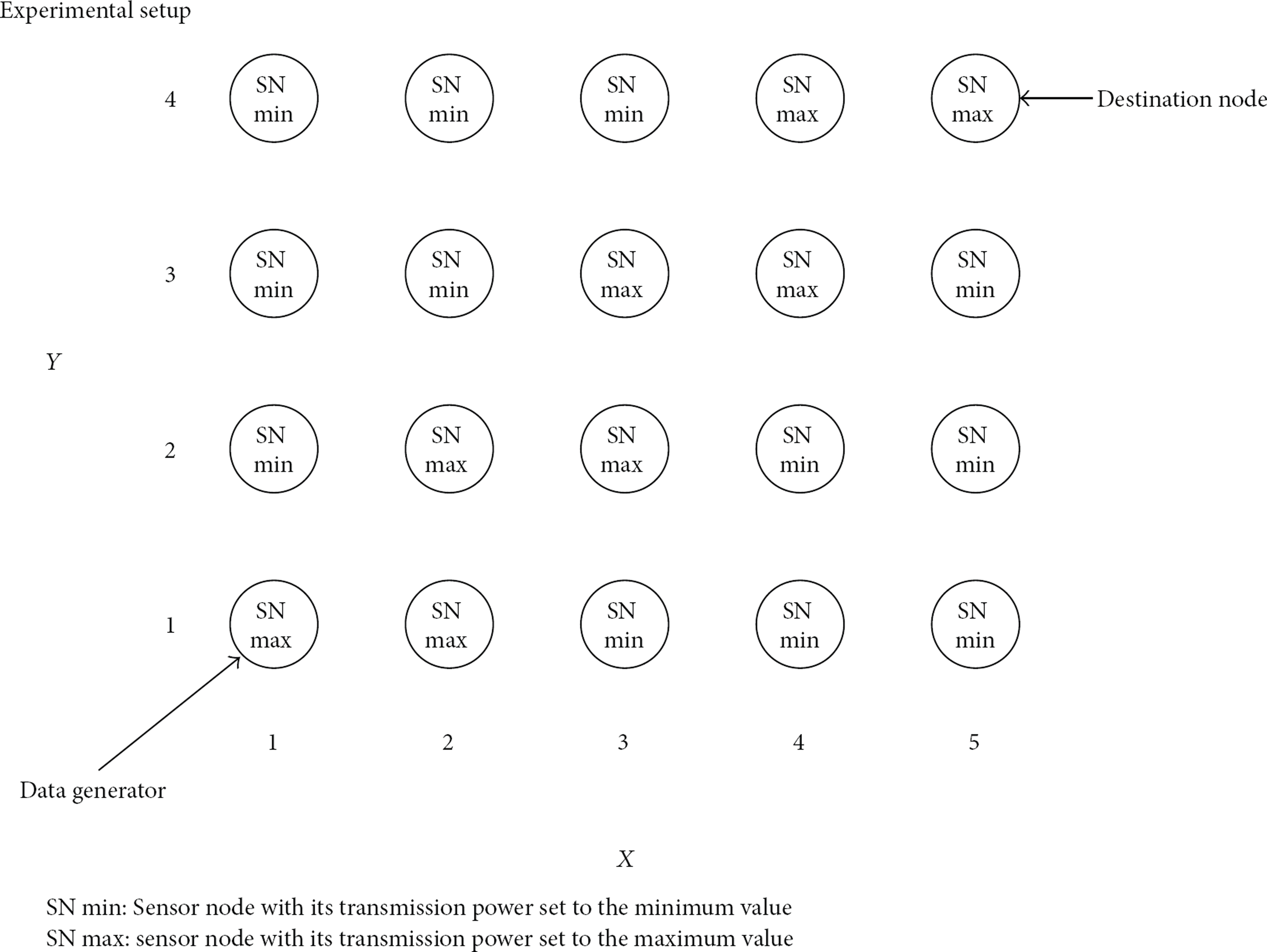
4.1. Physical Node Placement

Twenty (20) of these nodes were developed to implement the WSN testbed (see Figure 7). For the purposes of our investigation the SNs were placed in a rectangular grid (see Figure 6). In order to eliminate any bias in terms of routing protocol performance due to the physical architecture of the network, a rectangular grid was used. Although this is not representative of all real-world WSN deployments it provides a consistent and repeatable architecture for experiments. Furthermore, grid-like WNS deployments are attractive from a redundancy perspective [35] and considered to be quite typical for environmental sensing and office deployments [36]. To ensure proper communication between nodes, certain antenna dependent factors must be considered. From antenna theory, proper communication can only take place if communicating nodes fall within each other Fraunhofer region. In this region proximity of devices to the antenna does not affect its far-field radiation characteristics. It is easy to show that for the operating frequency of 2.45 GHz, and with the chosen antenna, the Fraunhofer region starts at approximately 0.3 m. As such, the nodes were placed 0.5 m apart.

Figure 6

Testbed hardware setup diagram.

Figure 7

Picture of the WSN testbed consisting of 20 nodes.

4.2. Radio Interference

It is well known that the 2.4 GHz band is one of the most hostile communication channels in the ISM environment. Results from [37] show that specifically IEEE 802.11b transmitters and microwave ovens negatively affect the performance of IEEE 802.15.4 networks. However, the interference can be mitigated by proper channel selection [38]. Suitable channels include 15, 20, 25, and 26, and for this reason the testbed operates its IEEE 802.15.4 network on channel 25.

4.3. Internode Communication Distance

Even when a SN is set to its lowest transmission power level ( $- 26.4$ dBm) it is simple to show that the communication range is in excess of 100 m (assuming ideal conditions). This is problematic for a testbed implementation due to physical space constraints within the laboratory environment. In order to mitigate this, each SN employs MAC filtering techniques to ensure that only neighbouring nodes can communicate. The MAC filtering technique employed ensures that no hardware modification is required if a more realistic testbed configuration is required.

4.4. Routing Framework

In order to ease the implementation of various routing schemes a simple framework was developed. This framework is based upon a distance vector routing protocol similar to the Routing Information Protocol (RIP) [39]. The three types of packets used by this protocol are listed as follows:

(i)

discovery packets;

(ii)

update packets;

(iii)

data packets.

Although only the source node actively generates data, other nodes in the network still forward data and maintain routing information. For our purposes only a single node actively transmits as this allows a clear observation of routing behaviour.

5. Experimental Setup

In order to conduct any experiment on the WSN testbed a specific chain of events must take place.

The specific setup steps (as shown in Figure 8) are

(i)

implementing a routing protocol;

(ii)

implementing a data generator;

(iii)

programming all SNs partaking in experiment;

(iv)

synchronising senor nodes;

(v)

clearing SN measurement memories.

Figure 8

Diagram detailing the experimental flow.

5.1. Control Experiment

To determine whether the entire testbed is functional an experiment is conducted during which each SN measures its own energy consumption. During this experiment the SNs actively discover nodes and maintain routing information, but no data is transmitted.

5.2. Validation Experiment

In order to perform validation on the testbed, a very simple experiment was conducted using a shortest path routing scheme. The details of this experiment are detailed hereon forth. A shortest path routing scheme was implemented by appending the existing routing framework as to include a cost metric based on the number of hops. As the name implies, the shortest route (based on the number of hops) is selected.

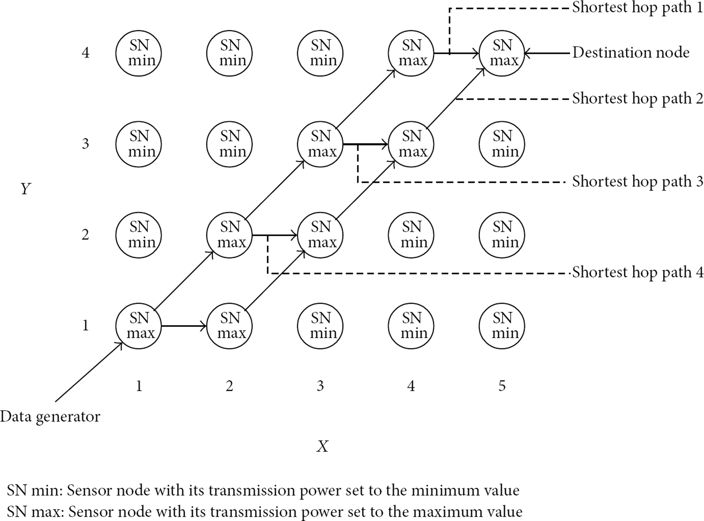
Data generation is accomplished by transmitting 200 packets, of 50 bytes each, once every 10 seconds from the source (nodes $1,1$ in Figure 8) to the destination node (nodes $4,5$ in Figure 6). With reference to Figure 9, the possible shortest hop paths are indicated. Note that several routes of equivalent length are possible; no specific mechanism is employed to decide between these alternatives.

Figure 9

Possible shortest hop paths.

As the shortest path routing protocol will select the same path continually, SNs on the selected path will be subjected to overuse. In order to ensure that the SNs remain alive for the duration of the experiment, the experiment was conducted for 60 minutes. The experiment was repeated three times in order to gather suitable amounts of data for statistical analysis. In order for the testbed to be validated one would expect the nodes located on the shortest path to have the highest energy consumption.

5.3. MTTP Experiment

As stated in Section 1, most of the active WSN routing protocol research is simulation based. It was postulated that this is due to the time efficiency afforded by simulation; however, one must be cognisant of the limitation of simulations, specifically as it pertains to the assumptions that the aforementioned simulation model is based on. For this reason, the MTTP routing scheme introduced in Section 2 will be implemented on the testbed. MPPT routing is selected as it serves as the foundation for many other proposed routing schemes (see Section 2).

As was the case with the validation experiment the existing routing framework is modified to include a transmission power cost metric that represents the total transmission energy cost associated with a route. As such, the MTTP routing protocol might select longer routes in an attempt to conserve energy. Thus, the end-to-end delay between source and destination nodes might be increased. The same data generator as that used for the shortest path routing protocol was used in the MTTPR experiment. The possible paths selected by the MTTP routing scheme are indicated in Figure 10.

Figure 10

Possible minimum total transmission power (MTTP) paths.

6. Results

The results of both the validation and research experiments are presented in this section.

6.1. General Results

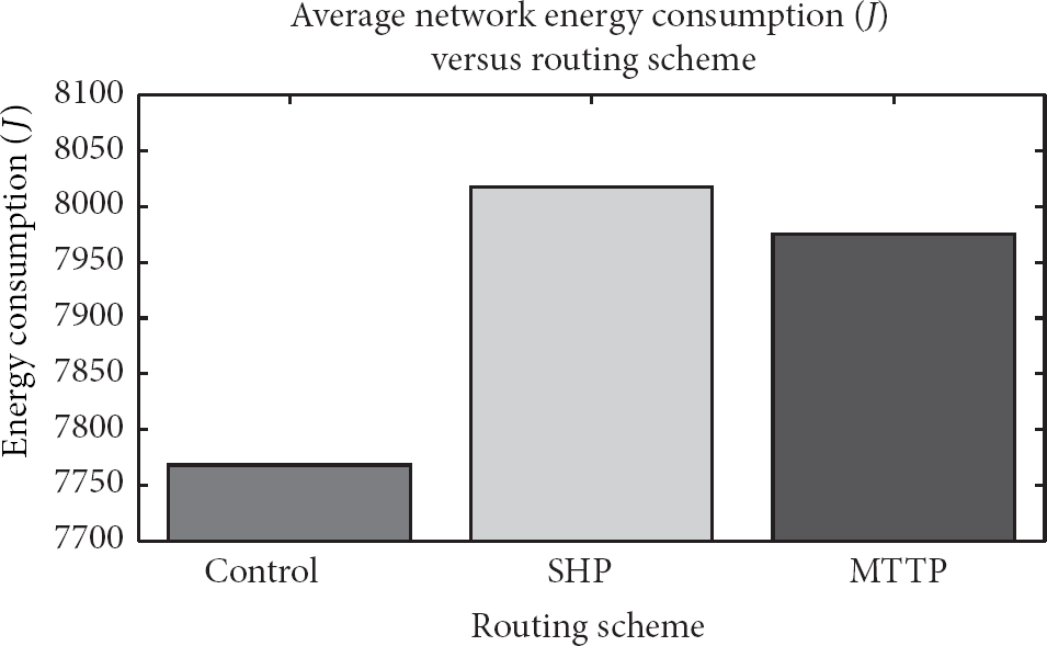
After completion of each of the individual experiments some statistical analyses were performed on the data to determine the accuracy of the results. For each of the experimental setups (control, SHP, and MTTP), the average network energy consumption was recorded and is graphed in Figure 11. Levene's test for homogeneity of variances is performed on this data to determine if the observed variances are due to random sampling. The values calculated by Levene's test are summarized in Table 6. A P value of less than $0.5$ indicates that the variances between the groups (control, SHP, and MTTP) are not due to random sampling.

Table 6

Levene's test for homogeneity of variances.

	MS effect	MS error	F	P
Total network energy consumption (J)	95.1968	37.4654	2.5409	0.1587

Figure 11

Plot of average network energy consumption $(J)$ versus routing scheme.

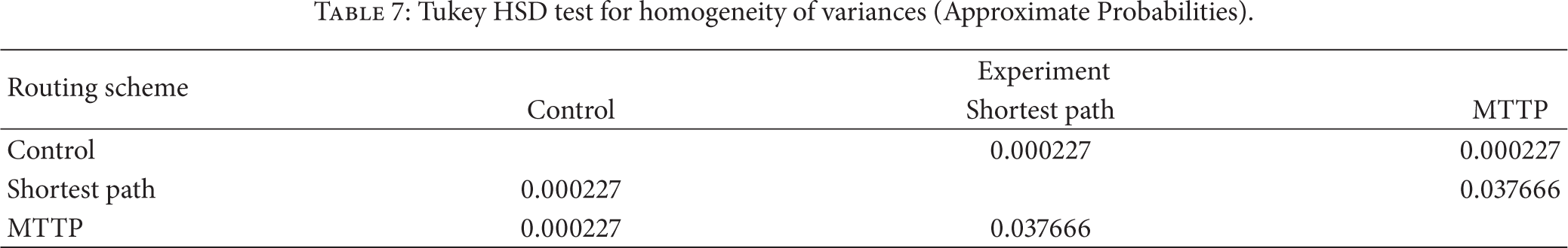
Additionally, a Tukey HSD test is performed to determine if the differences between routing schemes (none, SHP, and MTTP) are due to random chance. The Tukey approximate probabilities are provided in Table 7. All the P values are smaller than $0.05$ which indicates that there are statistically significant differences between all the experiments.

Table 7

Tukey HSD test for homogeneity of variances (Approximate Probabilities).

Routing scheme	Experiment
Routing scheme	Control	Shortest path	MTTP
Control		0.000227	0.000227
Shortest path	0.000227		0.037666
MTTP	0.000227	0.037666

6.2. Validation Results

A contour plot of the average network energy consumption for the shortest hop path routing scheme experiment can be seen in Figure 12. The nodes that consumed most of the energy are located on the path labelled shortest hop path 2 in Figure 9. This is the expected behaviour of the shortest path routing scheme. Therefore, the testbed is considered to produce valid data and is thus validated.

Figure 12

Contour plot of the average node energy consumption $(J)$ of the shortest hop path routing scheme.

6.3. MTTP Results

A contour plot of the average network energy consumption when MTTP routing scheme is used can be seen in Figure 13. The nodes that consumed the most energy are located on the path labelled MTTP path 1 in Figure 10.

Figure 13

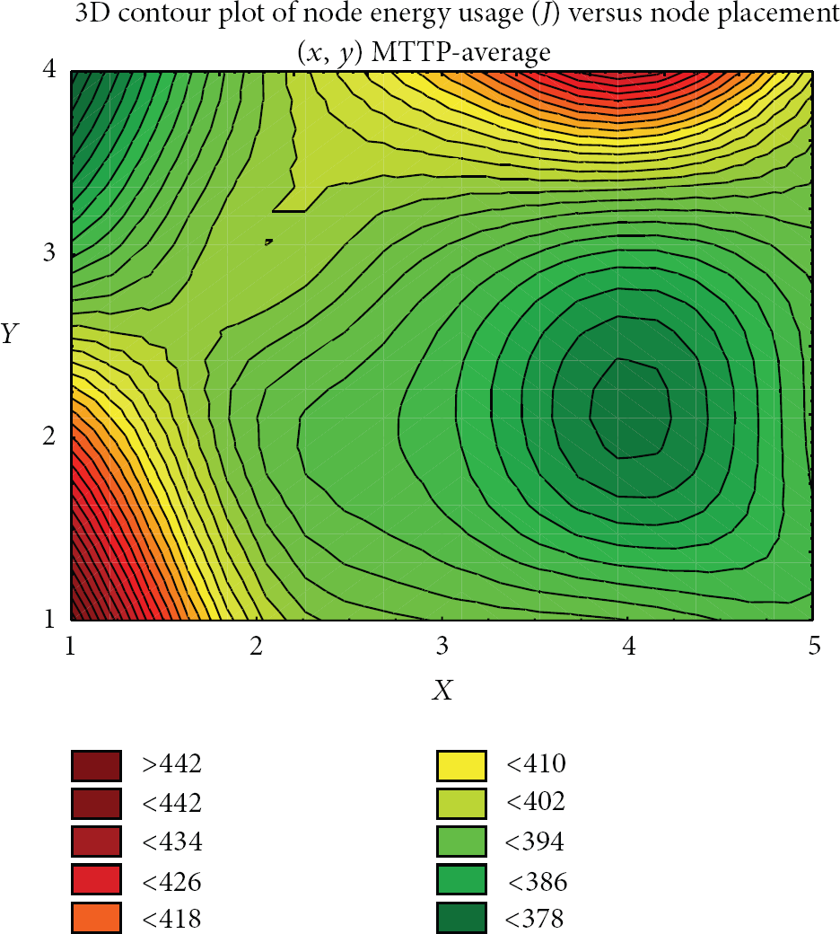
Contour plot of the average node energy consumption $(J)$ of the MTTP routing scheme.

7. Discussion

In Figure 11, the average energy consumption of the entire network for all three experiments can be seen. Although the MTTP scheme uses less energy than the shortest path benchmark, the saving is significantly less than expected. The RF transceiver used has a maximum output power of 19 dBm and a minimum transmission power of $- 26.4$ dBm. Thus, the MTTP scheme would expect a low-power node to use approximately 34673 times (45.4 dB) less energy than a high-power node.

Keeping in mind that the shortest path experiment made use of shortest path 2 in Figure 9, five full-power nodes were used. By a similar argument the MTTP scheme (which used MTTP path 1 in Figure 10) made use of 3 full-power nodes and 3 low-power nodes. Normalising individual node power to full-power nodes and assigning the expected energy saving of 45.4 dB to low-power nodes, it can be shown that MTTP should provide saving of almost $40 %$ for this experimental setup. However, the results (as in Figure 11) are in stark contrast to this, with the MTTP scheme offering an improvement of less than $1 %$ .

In order to explain this, the energy consumption characteristics of SNs versus transmission power settings need to be investigated. In Figure 14, the energy consumption of 10 SNs is shown for the idle, low-power ( $- 26.4$ dBm) transmission, and high-power (19 dBm) transmission states, respectively. Data was collected over a period of 20 minutes using a data generation scheme similar to that used during the experiments. Let $E_{\max} - E_{idle}$ denote the difference in energy consumption between a high-powered node and an idle node. Similarly, let $E_{\min} - E_{idle}$ denote the difference in energy consumption between a low-powered node and an idle node. Computing the ratio of $(E_{\max} - E_{idle}) / (E_{\min} - E_{idle})$ one finds that 2.82 is significantly less than the expected 45.4 dB. This can be attributed to the fact that low-power transceivers’ energy efficiency at low output power settings is significantly less than the energy efficiency at high output power settings.

Figure 14

A depiction of the energy consumption of 10 nodes at idle state, transmitting at minimum transmission power, and transmitting at maximum transmission power.

In an attempt to reduce the energy consumption of a WSN the MTTPR scheme replaces high transmission power hops with one or more low transmission power hops, in most cases expecting significant energy saving. However, due to the chip-level drain efficiency of low-power transceivers (typically employed in WSNs) this is not the case. In fact, the MTTPR scheme might even select routes that use more energy than a non-energy-aware routing protocol (such as shortest path) would use. This is because the MTTPR scheme replaces a single high-power hop with multiple low(er)-power hops but ignores the aforementioned output power dependent efficiency of the transceivers. It is clear that the MTTPR scheme can be modified to account for this. Currently the majority of simulation models used for the evaluation of the MTTPR scheme do not take this into account. This is also true for similar routing schemes such as MTTCP routing, MTRTP routing, and CMMBCR routing [13, 15, 40–43].

8. Conclusion

In this paper the development of a WSN sensor node capable of measuring its own energy consumption is detailed. Additionally, the authors investigated the fidelity of energy-aware WSN routing protocols, specifically MTTP routing. Although it was shown that MTTP routing offers some energy savings, as compared to non-energy-aware routing protocols, the saving was miniscule. The measured energy efficiency of MTTP routing and the theoretical expectations differ significantly. This is due to the chip-level drain efficiency of low-power RF transceivers, typically used in WSNs, not being taken into account by the MTTP routing scheme. In a worst-case scenario the MTTP scheme may even select a route which has a higher energy cost than a route selected by a non-energy-aware routing protocol (such as shortest path routing).

The transceiver's output power dependent energy efficiency negatively affects existing MPPT routing schemes’ expected energy savings. Routing schemes based on MTTP, such as MTTCP, MTRTP, and CMMBCR, are also affected. A simple modification to the MTTPR scheme would account for the observed phenomenon, but this modification would be unique for each transceiver. The simulation models used to compare energy-aware routing schemes will also need to be modified to take the transmission power dependent efficiency of SN transceivers into account.

Footnotes

Conflict of Interests

The authors declare that there is no conflict of interests regarding the publication of this paper.

References

Roundy

Steingart

Frechette

Wright

Rabaey

Karl

Wolisz

Willig

Power sources for wireless sensor networks

Wireless Sensor Networks 2004 2920

Berlin

Springer

1 17 Lecture Notes in Computer Science

Al-Regib

Distributed estimation in energy-constrained wireless sensor networks

IEEE Transactions on Signal Processing 2009 57 10 3746 3758

2-s2.0-70349640575

10.1109/TSP.2009.2022874

Anastasi

Conti

di Francesco

Passarella

Energy conservation in wireless sensor networks: a survey

Ad Hoc Networks 2009 7 3 537 568

2-s2.0-56449087483

10.1016/j.adhoc.2008.06.003

Pediaditakis

Mohajerani

S. H.

Boulis

Poster abstract: castalia: the difference of accurate simulation in WSN

Proceedings of the 4th European Conference on Wireless Sensor Networks (EWSN ′07)

January 2007

Delft, The Netherlands

Pham

H. N.

Pediaditakis

Boulis

From simulation to real deployments in WSN and back

Proceedings of the IEEE International Symposium on a World of Wireless, Mobile and Multimedia Networks (WoWMoM ′07)

June 2007

1 6

2-s2.0-47749089325

10.1109/WOWMOM.2007.4351800

Hurni

Braun

Fratta

Schulzrinne

Takahashi

Spaniol

Calibrating wireless sensor network simulation models with real-world experiments

Networking 2009 5550

Springer

1 13 Lecture Notes in Computer Science http://dblp.uni-trier.de/db/conf/networking/networking2009.html

Kotz

Liu

Newport

Yuan

Gray

R. S.

Elliott

Experimental evaluation of wireless simulation assumptions

Proceedings of the 7th ACM Symposium on Modeling, Analysis and Simulation of Wireless and Mobile Systems

October 2004

ACM Press

78 82

2-s2.0-27644464092

Watteyne

Molinaro

Richichi

M. G.

Dohler

From MANET to IETF ROLL standardization: a paradigm shift in WSN routing protocols

IEEE Communications Surveys and Tutorials 2011 13 4 688 707

2-s2.0-84857924325

10.1109/SURV.2011.082710.00092

Ren

Zhang

Lin

Ren

S. K. D.

EBRP: energy-balanced routing protocol for data gathering in wireless sensor networks

IEEE Transactions on Parallel and Distributed Systems 2011 22 12 2108 2125

2-s2.0-80055033920

10.1109/TPDS.2011.40

10.

Wheeler

Commercial applications of wireless sensor networks using ZigBee

IEEE Communications Magazine 2007 45 4 70 77

2-s2.0-34247560134

10.1109/MCOM.2007.343615

11.

Bhatia

Kaushik

A cluster based minimum battery cost AODV routing using multipath route for ZigBee

Proceedings of the 16th International Conference on Networks (ICON ′08)

December 2008

1 7

2-s2.0-66649095332

10.1109/ICON.2008.4772594

12.

IEEE standard for information technology—telecommunications and information exchange between systems—local and metropolitan area networks specific requirements part 15. 4: wireless medium access control (MAC) and physical layer (PHY) specifications for low-rate wireless personal area networks (lr-WPANs)

IEEE Std 2003 802. 15. 4-2003

IEEE

13.

Toh

C.-K.

Cobb

Scott

D. A.

Performance evaluation of battery-life-aware routing schemes for wireless ad hoc networks

Proceedings of the International Conference on Communications (ICC ′01)

June 2000

2824 2829

2-s2.0-0034851445

14.

Wang

Energy-efficient routing algorithms for wireless ad-hoc networks

Proceedings of the 18th Annual IEEE International Symposium on Personal, Indoor and Mobile Radio Communications (PIMRC '07)

September 2007

1 5

2-s2.0-44349164400

10.1109/PIMRC.2007.4394767

15.

Zhu

Wang

Model and protocol for energy-efficient routing over mobile Ad HOC networks

IEEE Transactions on Mobile Computing 2011 10 11 1546 1557

2-s2.0-80053113938

10.1109/TMC.2010.259

16.

Hellbruck

Pagel

Kroller

Bimschas

Pfisterer

Fischer

Using and operating wireless sensor network testbeds with WISEBED

Proceedings of the 10th IFIP Annual Mediterranean Ad Hoc Networking Workshop (Med-Hoc-Net '11)

June 2011

IEEE

171 178

2-s2.0-80052135275

10.1109/Med-Hoc-Net.2011.5970485

17.

Steyn

L. P.

Hancke

G. P.

A survey of wireless sensor network testbeds

Proceedings of the IEEE (Africon '11)

September 2011

1 6

2-s2.0-82955233777

10.1109/AFRCON.2011.6072072

18.

Tinynode 584 fact sheet v. 1. 1 25. 01. 2011 pca. Shockfish, http://www.tinynode.com

19.

Btnode datasheet

ETH Zurich, http://www.btnode.ethz.ch

20.

Baar

Will

Blywis

Hillebrandt

Liers

Wittenburg

Schiller

The scatterweb msb-a2 platform for wireless sensor networks

2008 TR-B-08-15 ftp://ftp.inf.fu-berlin.de/pub/reports/tr-b-08-15.pdf

21.

Telosb datasheet

Crossbow Technology, http://www.willow.co.uk

22.

Lotus datasheet

Mesmic, http://www.memsic.com

23.

Tmote sky datasheet

http://www.moteiv.com

24.

Micaz datasheet

Crossbow Technology, http://www.xbow.com

25.

G-node g301 whitepaper

SOWNet Technologies, http://www.sownet.nl/download/G301Web.pdf

26.

Sun spot technical datasheet

Oracle, http://www.sunspotworld.com/docs/Yellow/eSPOT8ds.pdf

27.

iSense core module 3 datasheet

Coalesenses, http://www.coalesenses.com

28.

Leopold

Sensor network motes: portability & performance [Ph.D. dissertation] 2007

Department of Computer Science Faculty of Science University of Copenhagen

29.

Waspmote homepage

libelium, http://www.libelium.com/products/waspmote/

30.

Krige

J. G. J.

Grobler

M. J.

Marais

A test-bed implementation of energy efficient wireless sensor network routing protocols

Proceedings of the Southern Africa Telecommunication Networks and Applications Conference (SATNAC ′12)

2012

31.

PIC24FJ128GA310 family datasheet

Microchip, 2011, http://www.microchip.com

32.

dsPIC/PIC24 Family Reference Manual—29. Real-time clock and Calendar (RTCC)

Microchip, 2013, http://www.microchip.com

33.

Krige

J. G. J.

Grobler

M. J.

Marais

A novel energy consumption ascertaining wireless sensor netowrk routing protocol test-bed

Proceedings of the Southern Africa Telecommunication Networks and Applications Conference (SATNAC ′13)

2013

TELKOM

309 313

34.

Yang

Microchip Wireless Media Access Controller MiMAC Microchip Technology

35.

Rao

G. S.

Vallikumari

A beneficial analysis of node deployment schemes for wireless sensor networks

International Journal of Advanced Smart Sensor Network Systems Systems 2012 2 2 33 43

36.

Takahara

Hassanein

On the robustness of grid-based deployment in wireless sensor networks

Proceedings of the International Wireless Communications and Mobile Computing Conference (IWCMC ′06)

July 2006

Vancouver, Canada

ACM

1183 1188

2-s2.0-34247324409

10.1145/1143549.1143786

37.

Huo

Bilen

C. C.

Zhang

Coexistence issues of 2.4 GHz sensor networks with other RF devices at home

Proceedings of the 3rd International Conference on Sensor Technologies and Applications (SENSORCOMM ′09)

June 2009

200 205

2-s2.0-70449492381

10.1109/SENSORCOMM.2009.40

38.

Tas

N. C.

Sastry

C. R.

Song

IEEE 802. 15. 4 throughput analysis under IEEE 802. 11 interference

Proceedings of the International Symposium on Innovations and Real Time Applications of Distributed Sensor Networks

2007

39.

Chen

Lin

Bai

Dai

A message interchange protocol based on routing information protocol in a virtual world

Proceedings of the 19th International Conference on Advanced Information Networking and Applications (AINA ′05)

March 2005

377 384

2-s2.0-33744493164

10.1109/AINA.2005.34

40.

Zhu

Qiao

Wang

A comprehensive minimum energy routing scheme for wireless ad hoc networks

Proceedings of the 23rd Annual Joint Conference of the IEEE Computer and Communications Societies (INFOCOM ′04)

March 2004

http://dblp.unitrier.de/db/conf/infocom/infocom2004.html

41.

Kim

luna aceves

J. J. G.

Obraczka

Carlos Cano

Manzoni

Power-aware routing based on the energy drain rate for mobile ad hoc networks

Proceedings of the 11th International Conference on Computer Communications and Networks

October 2002

10.1109/ICCCN.2002.1043126

42.

Gil

H. R.

Yoo

Lee

J. W.

Chung

C. W.

kwon Kim

Kim

Ling

T. W.

Song

K. H.

An on-demand energy-efficient routing algorithm for wireless ad hoc networks

Human.Society@Internet 2003 2003 2713

Springer

302 311 Lecture Notes in Computer Science http://dblp.unitrier.de/db/conf/human/human2003.html

43.

Misra

Banerjee

Mrpc: maximizing network lifetime for reliable routing in wireless environments

Proceedings of the Wireless Communications and Networking Conference (WCNC ′02)

March 2002

10.1109/WCNC.2002.993371

A Wireless Sensor Network Testbed for the Evaluation of Energy-Aware Routing Schemes

Abstract

1. Introduction

2. Background

2.1. Wireless Sensor Network

2.2. IEEE Standard 802.15.4

2.3. Energy-Aware Routing Schemes

2.4. Existing Sensor Nodes

3. Sensor Node Design

3.1. Microcontroller

3.2. Energy Measurement Unit

3.3. Communications Interface

3.4. Form Factor and Interconnects

3.5. Power Consumption

3.6. Measurement Accuracy

4. Testbed Setup

4.1. Physical Node Placement

4.2. Radio Interference

4.3. Internode Communication Distance

4.4. Routing Framework

5. Experimental Setup

5.1. Control Experiment

5.2. Validation Experiment

5.3. MTTP Experiment

6. Results

6.1. General Results

6.2. Validation Results

6.3. MTTP Results

7. Discussion

8. Conclusion

Footnotes

Conflict of Interests

References