Sage Journals: Discover world-class research

Abstract

We conducted a numerical study on the motion of a solid sphere settling under gravity in a viscous fluid using the lattice Boltzmann method combined with the smoothed profile method (SPM). The coupling of lattice Boltzmann fluid and a spherical particle is treated by introducing a body force term to the Boltzmann kinetic equation. For verification, we applied our numerical code to the simulation of flow over a static sphere and compared the results with previously published data. Later, we simulated the sedimentation process of a sphere inside a closed container. Our simulation results of the sphere's settling velocity and fluid velocity contours at various Reynolds numbers are in good agreement with the corresponding experimental results. Finally, we analyzed the accuracy of the present SPM for different forms for the smoothed profile function at various interface thicknesses and grid sizes.

1. Introduction

Colloidal suspension flows are very common in our daily life and have a wide range of applications in various fields such as chemistry, biology, medicine, and engineering [1, 2]. Many physicists have paid attention to the better understanding of the dynamics of colloidal suspensions through numerical simulations [3 –8]. Simulating the fluid flow of colloidal suspensions is very challenging because of the moving boundaries of the particles. Moving-boundary problems have generally been treated by using body-fitted or unstructured-grid methods. However, algorithms of these methods are usually complicated and are computationally expensive.

During the past two decades, the lattice Boltzmann method (LBM) has emerged as a powerful computational tool for solving fluid flow problems in colloidal suspensions [3, 4, 6, 9 –11] because of its advantages compared to the conventional Navier-Stokes (N-S) solvers based on finite-difference or finite-volume methods. Some of the advantages of LBM [12] are as follows: (1) pressure is computed by using an equation of state, which avoids having to solve the computationally expensive Poisson's equation, (2) the absence of convective terms in the Boltzmann equation (which causes fundamental numerical problems in N-S solvers) makes the LBM algorithm very simple, with all the operations fully local in time and space, and (3) since the data communication in the LBM algorithm is always local, it is very easy to implement the LBM algorithm in parallel computing applications.

Ladd [3, 4] was the first to employ LBM in simulating particulate suspension flows using the bounce-back (BB) rule to treat the no-slip boundary conditions (BCs) at fluid-solid interfaces. In this method, the surface of a colloidal particle is represented by a set of boundary nodes, which are chosen such that each boundary node is positioned at the middle of two fixed lattice grid points. A no-slip boundary condition (BC) is established by bouncing back the distribution functions coming from the fluid grid points to the solid nodes. Subsequently, many people have used Ladd's scheme in the simulation of colloidal suspension flows because of its easiness in implementation. Stratford et al. [9] implemented the BB rule in simulating colloidal suspensions in binary fluids. Nguyen and Ladd [10] used the BB rule to simulate particle suspension flows. They introduced an equation for lubrication force when the distance between two particles is very small. Iglberger et al. [11] used a modified BB rule, that is, Ladd's scheme with an interpolated BB scheme, to simulate the behavior of particle agglomerates in a fluid flow. Even though Ladd's scheme can be applied to many colloidal flow applications, the main drawback of this scheme is that the solid boundary of a moving particle does not move continuously in time and space, which causes fluctuations in the fluid flow velocity at fluid-solid interfaces.

Another approach for simulating the fluid flow around a moving body on a fixed Cartesian grid system is the immersed boundary method (IBM) proposed by Peskin [13, 14]. In IBM, the particle boundary is represented with a finite number of Lagrangian nodes, and a fixed Eulerian mesh is used to compute the fluid flow; the no-slip condition is enforced by adding an artificial body force to the fluid grid points. Various approaches to calculating the body force can be found in the review article by Mittal and Iaccarino [15]. To update the velocity and position of the particles, the opposite of the body force is added to Newton's equation of motion in order to conserve the total momentum of the fluid-particle system. IBM combined with LBM is one of the successful methods for incorporating the no-slip condition in moving-boundary problems. Feng and Michaelides [16] combined IBM with LBM for the first time to utilize the advantages of both. Subsequently, many people have applied the immersed boundary LBM to a number of problems, for example, the sedimentation process of large numbers of particles in a host fluid [17], deformable capsules and red blood cells in channel flows [18, 19], and simulation of particulate suspension flows [20]. Even though IBM resolves the problem of Ladd's scheme (fluctuations in fluid velocity), the main drawback of this method is that it requires complicated interpolation functions and needs global data communication between the Eulerian and Lagrangian nodes. This restricts the utilization of the local nature of LBM in parallel computations. Recently, Nie and Lin [21] used the combination of LBM and the so-called direct-forcing factious domain method to simulate the sedimentation of elliptical particles in a vertical channel. This method, however, also needs interpolation functions to transfer data between the Eulerian and Lagrangian nodes as in IBM.

To avoid using complicated interpolation functions and the need for global data communications, many later researchers focused on direct-forcing methods such as the fluid-particle dynamics method [5] and the smoothed profile method (SPM) [7]. Jafari et al. [22] developed LBM based on SPM to predict the dynamic behavior of colloidal dispersions. The advantage of SPM over IBM is that all the operations in the SPM method are localized to a grid point as the same computational mesh is used for fluid and particles, and so LBM combined with SPM can be easily implemented in parallel computing applications. In their work, Jafari et al. [22] conducted simulations of two-dimensional (2D) flow problems using LBM combined with SPM, but as far as we know no simulation results have been reported for three-dimensional (3D) problems. In the present work, we extended the scheme of Jafari et al. to a 3D problem, simulation of the sedimentation process of a sphere inside a closed container. We also analyzed the effect of different formulas for the smoothed profile function on the accuracy of SPM.

The remainder of this paper is arranged as follows. A brief description of the numerical method used in the present work is given in Section 2. The numerical results are provided in Section 3; in the first part, we present the simulation results of flow over a static sphere; then, the results obtained from the simulation of the sedimentation process of the sphere are given, and the results of the accuracy analysis of the SPM are provided in the last part. Finally, the concluding remarks of the study are given in Section 4.

2. Numerical Method

In this work, we employ LBM to compute flow field caused by the motion of particles in the host fluid. In LBM, the fluid density and velocity are calculated from the fluid-particle density distribution functions, f_n(x, t), which are obtained by numerically solving the Boltzmann kinetic equation on a discrete lattice mesh [23]. Here f_n(x, t) corresponds to the probability of finding a particle at a lattice location x and at a time t having a discrete velocity c_n (n = 0,1, …, b), which is chosen such that after the time step Δt the particle arrives at the nth neighboring grid point [24]. The subscript n denotes the link number of a lattice. In this paper, we work with a cubic lattice consisting of 19 velocity vectors (b = 19) in 3D space (D3Q19 lattice [12]). The lattice Boltzmann equation with an external body force term [22] is given by

f_{n} (x + c_{n} Δ t, t + Δ t) = f_{n} (x, t) - \frac{1}{λ} (f_{n} (x, t) - f_{n}^{eq} (x, t)) + \frac{w_{n} Δ t}{c_{s}^{2}} (f^{fl} (x, t) \cdot c_{n}),

(1)

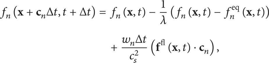
where λ is the relaxation time, w_n is the weighing function of c_n, c_s is the speed of sound, and f^fl(x, t) is the hydrodynamic force due to the interaction between the particles and the fluid. To compute f^fl(x, t), we use a smoothed profile method. After getting f_n(x, t), the fluid density, ρ(x, t), and the fluid velocity, u(x, t), are obtained from

ρ (x, t) = \sum_{n = 0}^{b} f_{n}, u (x, t) = \frac{1}{ρ} \sum_{n = 0}^{b} f_{n} c_{n} .

(2)

2.1. Calculation of Body Force Term

In SPM, in order to evaluate f^fl(x, t), one uses a smoothed profile function (also known as an indicator/concentration function), φ_i(x, t), to identify the position of a particle i. φ_i(x, t) values are defined in such a way that φ_i = 0 in the fluid domain, φ_i = 1 in the particle domain, and φ_i varies smoothly from 0 to 1 at the interface between the fluid and solid. There are several ways to calculate φ_i values. In the present work, we use the following function:

ϕ_{i} (x, t) = f (R_{i} - |x - X_{i} (t)|),

(3a)

f (r) = \{\begin{cases} 0, & r < - \frac{ξ_{i}}{2}, \\ \frac{1}{2} (\sin (\frac{π r}{ξ_{i}}) + 1), & |r| < \frac{ξ_{i}}{2}, \\ 1, & r > \frac{ξ_{i}}{2}, \end{cases}

(3b)

where R_i, X _i(t), and ξ_i are the radius, position, and the interface thickness of the particle i. A smoothly distributed concentration field of all the particles, φ( x , t), can then be obtained by summing all the φ_i( x , t) values of N particles:

ϕ (x, t) = \sum_{i = 1}^{N} ϕ_{i} (x, t) .

(4)

After finding the particle concentration field φ( x , t), we get the body force term in (1) from

f^{fl} (x, t) = \frac{ϕ (x, t) [u_{p} (x, t) - u (x, t)]}{Δ t},

(5)

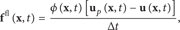
where u and u _p( x , t) are the velocity field of the fluid and particle, respectively. In the above equation the velocity field, φu_p, of all the particles can be computed by

ϕ (x, t) u_{p} (x, t) = \sum_{i = 1}^{N} ϕ_{i} (x, t) [V_{i} (t) + ω_{i} \times (x - X_{i} (t))],

(6)

where V _i(t) and ω_i are the translational and rotational velocities of the particle i.

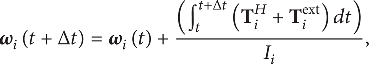
2.2. Updating Particles Positions and Velocities

The relative motion of particles submerged in fluid causes hydrodynamic force, $F_{i}^{H}$ , and torque, $T_{i}^{H}$ , on the particles. Equations for $F_{i}^{H}$ and $T_{i}^{H}$ can be derived from the conservation of momentum between the particles and the fluid. Based on the momentum exchange during the time step Δt, we can write the equations for hydrodynamic force and torque as follows:

\int_{t}^{t + Δ t} F_{i}^{H} d t = \int_{V_{i}}^{} ρ (x, t) ϕ_{i} (x, t) [u (x, t) - u_{p} (x, t)] d V_{i},

(7a)

\int_{t}^{t + Δ t} T_{i}^{H} d t = \int_{V_{i}}^{} ρ (x, t) ϕ_{i} (x, t) [x - X_{i} (t)] \times [u (x, t) - u_{p} (x, t)] d V_{i},

(7b)

where V_i is the volume of the particle i.

After finding $F_{i}^{H}$ and $T_{i}^{H}$ , the translational and rotational velocities of each particle are updated from Newton's second law:

V_{i} (t + Δ t) = V_{i} (t) + \frac{(\int_{t}^{t + Δ t} (F_{i}^{H} + F_{i}^{ext}) d t)}{M_{i}},

(8a)

ω_{i} (t + Δ t) = ω_{i} (t) + \frac{(\int_{t}^{t + Δ t} (T_{i}^{H} + T_{i}^{ext}) d t)}{I_{i}},

(8b)

where $F_{i}^{ext}$ and $T_{i}^{ext}$ are the external forces (such as gravity, electrophoretic, magnetic) and torque acting on the particle i, and M_i and I_i are the mass and moment of inertia of the particle. After obtaining the translational and rotational velocities, the positions of the particles can be updated from

X_{i} (t + Δ t) = X_{i} (t) + \int_{t}^{t + Δ t} V_{i} (t) d t .

(9)

3. Simulation Results

3.1. Steady Flow Past a Static Sphere

To validate our code, we simulated the flow over a stationary sphere located within a rectangular channel (Figure 1) and compared our simulation results with previously published data. The length, height, and width of the domain are taken as L = 35a, H = 10a, and W = 10a, respectively, where a is the sphere radius. The sphere is placed at a distance 15a from the inlet of the domain, far enough from the inlet to minimize the entrance effect. A uniform velocity profile is given as the inlet (at y = 0) BC thorough the following BB scheme:

f_{\bar{n}} (x_{b}, t) = f_{n} (x_{f}, t) + \frac{2 w_{n} ρ_{in}}{c_{s}^{2}} (U_{in} \cdot c_{\bar{n}}),

(10)

where $f_{\bar{n}} (x_{b}, t)$ is the density distribution function of a fluid particle travelling from the boundary node, x _b, to the fluid node, x _f, with lattice velocity $c_{\bar{n}}$ , which is in the opposite direction of c _n. Further, ρ_in and U _in are the density and velocity, respectively, of the fluid at the inlet.

Figure 1:

Cross-sectional view of the numerical setup used for simulating flow over a static sphere at the central (a) yz-plane and (b) xz-plane (not to scale).

The BCs at outlet (y = L) and at side (x = 0 and x = W) and top (z = 0 and z = H) walls are treated with a second-order extrapolation scheme proposed by Mei et al. [25], which can be explained in more detail as follows. Suppose i, j, and k are the indices of the computational grid in x-, y-, and z-directions, respectively. The BCs for f_n's at y = L are set as

f_{n} (i, n_{y} + 1, k) = 2 f_{n} (i, n_{y}, k) - f_{n} (i, n_{y} - 1, k),

(11)

where j = n_y + 1 is the boundary node at y = L. Also, we need to set the velocity at j = n_y as

u (i, n_{y}, k) = u (i, n_{y} - 1, k) .

(12)

This extrapolation scheme allows the fluid flow to leave the boundary and helps to reduce the effect of boundaries on the flow field and drag force. The BCs at side and top walls are treated in the same way as in (11) and (12).

The initial fluid density and velocity in all our simulations are taken as ρ = 0 and u = 0, respectively. We set the sphere radius a = 4, the fluid kinematic viscosity ν = 0.1, and the interface thickness ξ = 0.25 in the lattice units (LU). We compared the velocity profiles obtained from our simulation with the previously published data at Reynolds number, Re = 10; here, Re is defined as Re = 2U_ina/ν. Figure 2 shows the variation of axial velocity profile, u_y, evaluated at the central yz-plane along the z-axis (Figure 2(a)) and that along the y-axis (Figure 2(b)). Our simulation results are in good agreement with the results from Mei et al. [25], who used an interpolated BB scheme to enforce the no-slip BC on the sphere surface.

Figure 2:

Variation of axial velocity profile, u_y, with the (a) position along the z-axis and that with the (b) position along the y-axis.

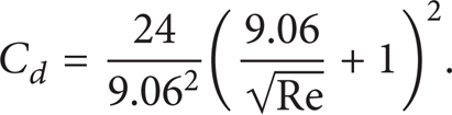
We also compared our simulation result of variation of the sphere's drag coefficient, C_d, with Re with an empirical relation [26]:

C_{d} = \frac{24}{9.0 6^{2}} {(\frac{9.06}{\sqrt{Re}} + 1)}^{2} .

(13)

C_d values of our simulation results are obtained from the equation for the drag force on the sphere, F_d = ρU_in²C_dA/2, where A = πa² is the sphere's reference area. We used (7a) to compute F_d (here F_d is the y-component of $F_{i}^{H}$ ). Figure 3 shows the variation of the drag coefficient of the sphere with Reynolds number, for Re ranging from 1 to 100. The symbols in the figure denote our simulation results, and the solid line denotes the results from the empirical relation. Re is varied by changing the U_in values while keeping the kinematic viscosity at ν = 0.04 (in LU) when Re < 40 and at ν = 0.01 when Re > 40. The reason for choosing two different values for ν is explained as follows. The accuracy of LBM results depends on the Mach number, Ma (ratio of maximum flow velocity in the simulation and the speed of sound, $c_{s}^{} = 1 / \sqrt{3}$ in LU). In order to obtain accurate results using the standard LBM, Ma should be very low (Ma ≪ 1). If we choose ν = 0.04 for Re > 40, the Mach number in our simulations is in the order of 1, which is not a good choice to get accurate results. On the other hand, if ν = 0.01 is chosen when Re < 40, the time taken to reach the convergent solution becomes longer. So, we choose two different values for ν depending on the Reynolds number. As is seen from Figure 3, our simulation results agree very well with the empirical data in particular at low Re.

Figure 3:

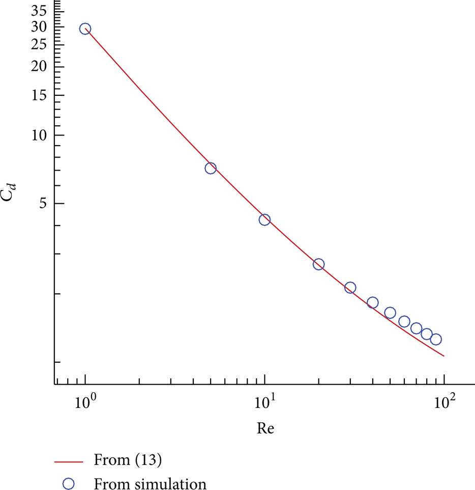
Comparing the variation of drag coefficient of the sphere, C_d, with the Reynolds number, Re, obtained from theoretical equation, (13), and that from simulation.

From this validation, we can say that our 3D numerical code is accurate and reliable. This encouraged us to perform simulations on moving-boundary problems using LBM combined with SPM. We selected the problem of the sedimentation of a sphere due to gravity, as it is one of the standard benchmark problems to assess the validity of a proposed numerical method for the moving-boundary cases.

3.2. Simulation of Falling Sphere under Gravity

In this section, we present the numerical results obtained from the simulation of the motion of a solid sphere settling in a viscous fluid at rest under the influence of gravitational force. Figure 4 shows the simulation setup employed in the present work. All the simulations are carried out inside a closed box filled with a viscous fluid. The simulation parameters (Table 1) together with the box size are set to be the same as those of ten Cate et al. [26], who conducted experiments on a sphere falling freely in a silicone oil using the particle image velocimetry technique. After a sphere having a radius a = 7.5 mm and a density ρ_s = 1120 kg/m³ is released at a distance of 120 mm from the bottom wall of the container, it settles downwards due to gravitational force:

F_{g} = \frac{4}{3} π a^{3} (ρ - ρ_{s}) g k,

(14)

where g = 9.8 m/s² is the gravitational acceleration and k is the unit vector in the z-direction. Simulations are carried out at four different Reynolds numbers as given in Table 1. Here, Reynolds number is defined based on the steady state settling velocity of a sphere, u_∞, in an infinite medium. Re in our simulations is varied by changing the viscosity of the fluid. The simulation domain is divided into 131 × 131 × 209 lattice grid points in x-, y-, and z-directions, respectively. So, the radius of the sphere is a = 9.75 in LU. We applied the standard midplane BB [(10) with U _in = 0] to satisfy the no-slip BC at the solid walls of the box, and the no-slip BC on the sphere surface is treated by SPM. We take the interface thickness of the smoothed profile function as ξ = 0.25. It is worth mentioning that our simulation setup differs from the corresponding experimental one on two points: (1) we assumed the top wall of the domain to be a solid instead of a liquid free surface, as applying the free-surface condition is very difficult in LBM and (2) we stop the simulation when the dimensionless gap, G, between the sphere and the bottom wall of the domain is less than the unit lattice spacing.

Table 1:

Parameters used in the present simulation. The parameters presented in the first three columns are taken from ten Cate et al. [26].

Reynolds number, Re	Fluid density (kg/m³)	Viscosity (Ns/m²)	Simulation time step, Δt (s)	Velocity ratio, u_{max ⁡}/u_∞

1.5	970	373	Δt = 2 × 10^{− 4}	0.8915
4.1	965	212	Δt = 3.5 × 10^{− 4}	0.9521
11.6	962	113	Δt = 4.5 × 10^{− 4}	0.9558
31.9	960	58	Δt = 5.9 × 10^{− 4}	0.945

Figure 4:

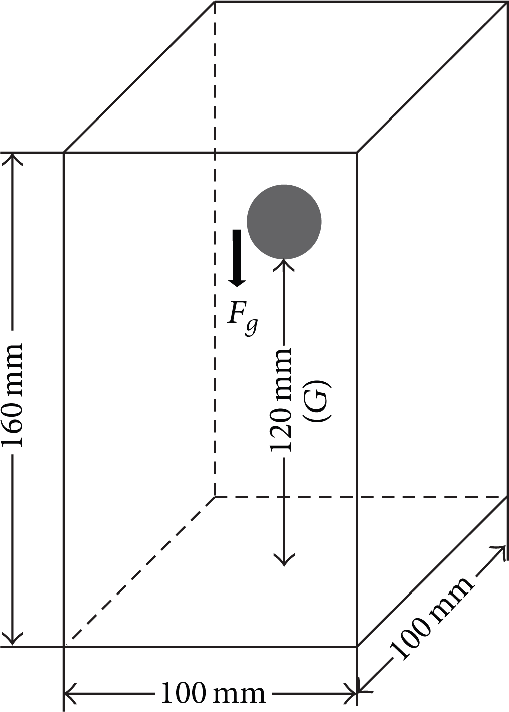
Simulation setup used for simulating the motion of a single sphere settling due to the gravitational force, F _g. G is set initially at 120 mm as shown but varies in time.

Figure 5 shows the variation of the gap normalized by the sphere diameter, G/(2a), and the sedimentation velocity of the sphere with time t for different Re; the solid lines represent our numerical results, the symbols the experimental results given by ten Cate et al. [26], and the dashed lines the numerical results obtained from IBM by Suzuki and Inamuro [27]. Our results for sedimentation velocity and trajectory of the sphere are in good agreement with the experimental results at all Re values. We can also notice from Figure 5 that our simulation results are in better agreement with the experimental results than the data of Suzuki and Inamuro [27] given by IBM, even though we used a coarser grid system compared to Suzuki and Inamuro, who used 200 × 200 × 320 lattice grid points.

Figure 5:

Variation of (a) the sphere trajectory and (b) the sedimentation velocity with time at different Reynolds numbers. Solid lines indicate our numerical results, symbols the experimental results [26], and dotted lines the results obtained from IBM [27].

As seen from Figure 5, the velocity of the sphere gradually increases until it reaches the steady state, where the drag force on the sphere equals its gravitational force. As the sphere approaches the bottom of the box, it starts to decelerate, because when the bottom wall is approached, the upward (buoyant) force on the sphere overtakes the gravitational force since the squeezing of the fluid between the sphere and the bottom wall of the box increases the fluid pressure there. We also compared the flow field obtained from our simulation results with the experimental results. Figure 6 shows the comparison of the flow field contours obtained from our simulations (Figure 6(a)) and those obtained from the experiments (Figure 6(b)) at different Re. The contours are plotted when the sphere's center position is at one diameter away from the bottom wall, that is, when G/a = 1. At all values of Re, the simulated velocity magnitude contours show good agreement with the experimental results. Squeezing of the liquid between the sphere and the bottom wall causing the outward flow is also well described.

Figure 6:

Comparison of flow field contours at different Re obtained from the present simulations (a) and experiments [26] (b). Contours are plotted when the sphere center position is one diameter away from the bottom wall.

We also compared the maximum settling velocity of the sphere, u_{max ⁡}, with u_∞. To calculate u_∞, we first use (13) for finding C_d for a given Re and then u_∞ is obtained from the drag force, F_d = ρu_∞²C_dA/2, where F_d is set as the gravitational force. The ratio u_{max ⁡}/u_∞ obtained in this way at different Re is listed in Table 1, which shows that the ratio u_{max ⁡}/u_∞ decreases as Re is decreased at Re less than 11.6. The reason for the significant deviation of u_{max ⁡}/u_∞ from 1 at low Re (Table 1) can be explained with the help of Figure 7, which shows the contour plot of the magnitude of the flow velocity normalized with u_∞ at different Reynolds numbers when the sphere attains u_{max ⁡} in each case. We can see from Figure 7 that the lateral extension of the flow profile caused by the sphere's motion is enhanced as Re is decreased indicating more pronounced interaction between the motion of the sphere and the stationary side wall at lower Re. This means that the sphere moving at lower Re experiences larger drag force due to the container side wall effect. On the other hand, as Re is increased the drag force coefficient obtained from our simulation begins to surpass the theoretical one, (13), from Re = 30 as shown in Figure 3. This seems to be the main reason for the lower value of u_{max ⁡}/u_∞ at Re = 31.9 than that at Re = 11.6.

Figure 7:

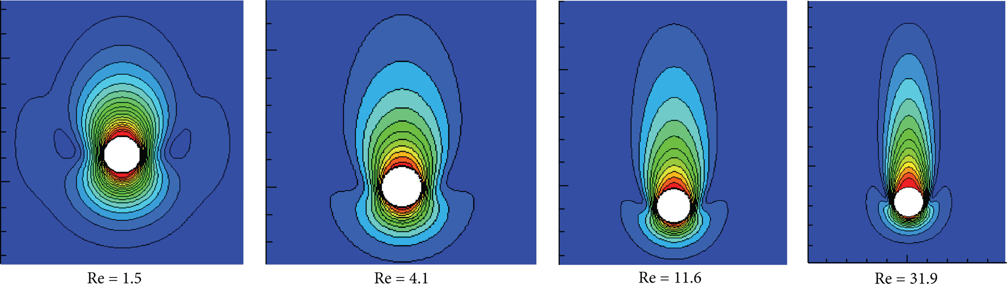
Plots of the fluid flow contours at different Re when the sphere attained u_{max ⁡} at each Re case.

3.3. Analysis of the Accuracy of SPM

We also analyzed the effect of the various formulas proposed by Nakayama and Yamamoto [7] to evaluate the smoothed profile function on the accuracy of SPM. For the present accuracy-analysis study we have chosen the case of Re = 11.6. As already mentioned, in this work, we mainly use (3b) to calculate the smoothed profile function, φ_i( x , t), which will be referred to as C1 hereafter. There are many other alternative choices for calculating φ_i( x , t) values. One of the possible choices is (C2) [7]

ϕ_{i} (x, t) = f (|x - X_{i} (t)|),

(15a)

\begin{matrix} f (r) = \frac{h [(R_{i} + ξ_{i} / 2) - r]}{h [(R_{i} + ξ_{i} / 2) - r] + h [r - (R_{i} - ξ_{i} / 2)]}, \\ h (s) = \{\begin{cases} 0, & s \leq 0, \\ \exp (- \frac{Δ^{2}}{s^{2}}), & s > 0, \end{cases} \end{matrix}

(15b)

where Δ is the lattice spacing. Another possible choice (C3) for evaluating φ_i( x , t) values is [7]

ϕ_{i} (x, t) = \frac{1}{2} [\tanh (\frac{R_{i} - |x - X_{i} (t)|}{ξ_{i}}) + 1] .

(16)

Figure 8 shows the variation of sedimentation velocity of the sphere with time when φ_i values are evaluated with different choices. We set the interface thickness and sphere radius at ξ = 0.5 and a = 7.5, respectively. The results obtained with C1 and C2 are in better agreement with the experimental results compared to those obtained with C3. The reason for this can be explained using Figure 9, which shows the sketch of the smoothed profile functions obtained from different choices. When φ_i values are evaluated using C1 and C2, there is a clear separation between the solid, fluid, and interfacial domains, whereas the separation of the three domains is unclear when C3 is used. In Figure 8, we can see that the results obtained from using C1 and C2 are almost the same as each other since the smoothed profiles given by these two choices are identical to each other as depicted in Figure 9. We also measured how drag force acting on the sphere, F_d, varies with time (Figure 10) when different choices are used for φ_i. We checked this because the stability of the numerical scheme depends on how smoothly the drag force varies with time. Even though C2 gives accurate results, the amount of fluctuation in drag force obtained with C2 is very high compared to that found with C1 and C3.

Figure 8:

Comparison of variation of sedimentation velocity of the sphere with time at Re 11.6 when φ_i values are obtained with different choices. Here, C1, C2, and C3 correspond to the use of (3a), (3b), (15a), (15b), and (16), respectively, for calculating φ_i values.

Figure 9:

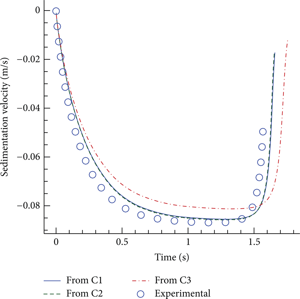
Sketch of the smoothed profile function obtained from different choices.

Figure 10:

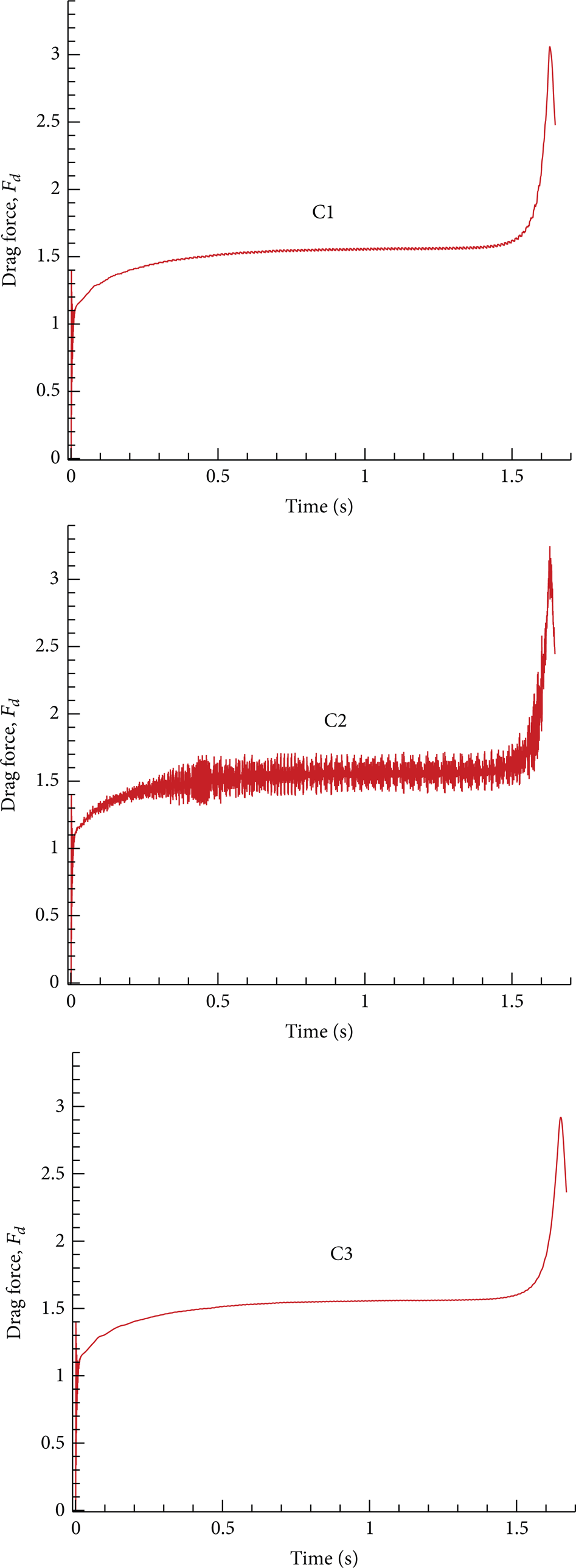
Variation of the drag force acting on the sphere, F_d, with time obtained from different choices at ξ = 0.25.

We compared the numerical error and the rms value of the fluctuations in drag force obtained with three different choices for the smoothed profile function at various values of the interface thickness and grid size. The numerical error is calculated from the formula $\sum_{t} {(u_{sim, t} - u_{\exp, t})}^{2}$ , where u_{sim, t} and u_{exp ⁡, t} are the sedimentation velocity of the sphere at time t obtained from the simulation and the experiment, respectively. Similarly, we calculated the rms value of fluctuations in the drag force from

F_{d}^{rms} = \sqrt{\sum_{t_{s}}^{t_{e}} \frac{{(F_{d, t}^{} - {\bar{F}}_{d, t}^{})}^{2}}{N}},

(17)

where $F_{d, t}^{}$ and ${\bar{F}}_{d, t}^{}$ are the instantaneous and average value of the drag force at time t, respectively, and N is the total number of data points in a time interval, t_e − t_s. ${\bar{F}}_{d, t}^{}$ values are evaluated from a linear regression model of $F_{d, t}^{}$ data points in the interval, t_e − t_s. We have chosen a specific time interval such that the variation of F_d versus t is almost linear in terms of the locally averaged drag force ${\bar{F}}_{d, t}^{}$ during the interval t_e − t_s, say from t_s = 1.25 s to t_e = 1.35 s.

Figure 11 shows the variation of the numerical error (Figure 11(a)) and F_d^rms (Figure 11(b)) with the interface thickness when φ_i values are evaluated from three choices. When C2 is used, the numerical error is almost unaffected by the interface thickness but F_d^rms varies significantly with ξ showing high fluctuations of F_d at lower values of ξ. When C3 is used, the error increases dramatically with ξ. However, fluctuations in drag force obtained with C3 remain quite low regardless of ξ. On the other hand, C1 provides both small errors and relatively low-level fluctuations in F_d. From this comparison, we can say that C1 is the best choice among the three in view of the reasonable accuracy of the results as well as relatively weak fluctuation.

Figure 11:

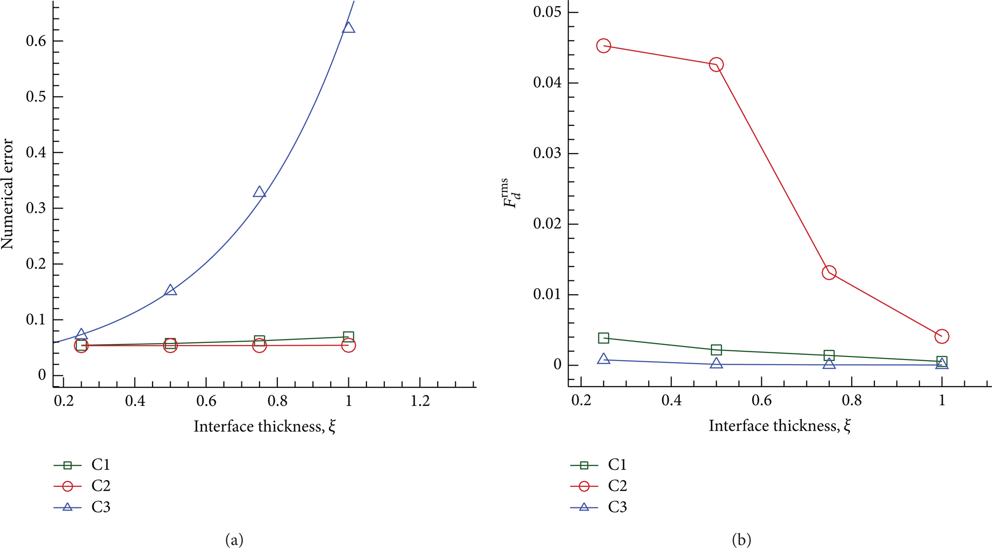
Variation of (a) numerical error and (b) rms value of drag force, F_d^rms, with the interface thickness when φ_i values are obtained with different choices.

We also checked the effect of grid size on the numerical error and F_d^rms by considering different radii of the sphere, a = 5.25, 7.5, and 9.75 in LU. Note that here we have only changed the sphere radius in dimensionless units but adjusted the grid size to keep the simulation domain size the same in physical units. In order to remove the effect of the truncation in the numerical integration of (8a), (8b), and (9) on the numerical error, the simulation time step in real units is kept the same in all cases. Figure 12 shows the instantaneous settling velocities of the sphere obtained for different grid sizes. The interface thickness is kept at ξ = 0.25 and φ_i values are evaluated by using C1. From Figure 12, it is clear that the accuracy of the numerical method improves with smaller grid sizes.

Figure 12:

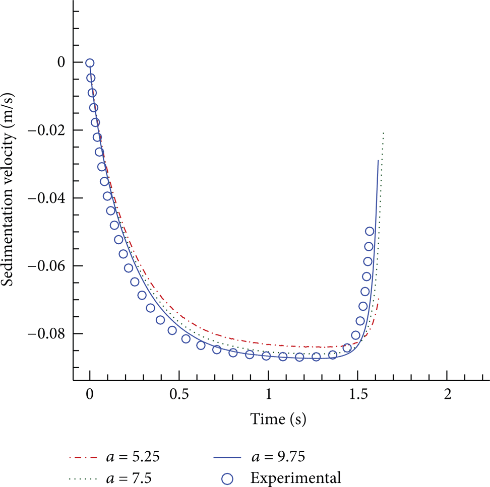
Comparison of variation of sedimentation velocity of the sphere with time at Re 11.6 when different grid sizes are used.

Finally, we compared the variation of the numerical error (Figure 13(a)) and F_d^rms (Figure 13(b)) with the grid size for three choices for φ_i. Obviously, the numerical error decreases with the grid size in all the three cases, though the error is almost the same for the case of C1 and C2 (Figure 13(a)). The error obtained with C3 is always higher than that obtained with the other choices. On the other hand, F_d^rms value obtained with C2 is again much higher than those given by C1 and C3. As expected; however, F_d^rms value decreases sharply as the grid is refined.

Figure 13:

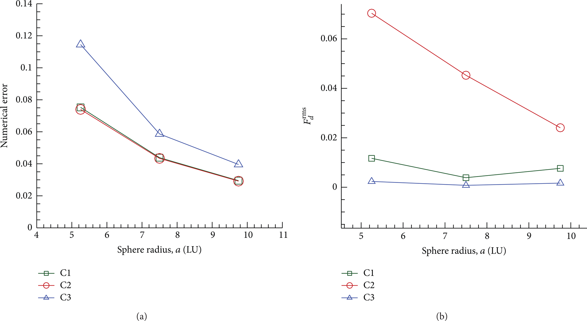
Variation of (a) numerical error and (b) rms value of drag force, F_d^rms, with the grid size when φ_i values are obtained with different choices.

4. Conclusions

In this work, we developed a FORTRAN code based on the lattice Boltzmann method combined with a smoothed profile method (SPM) to numerically investigate the sedimentation process of a sphere in a viscous fluid. Firstly, we simulated a steady flow over a static sphere and validated our numerical code by comparing our simulation results with previously published data. We then carried out simulations on a single sphere settling under gravity inside a closed container. Our simulation results of the sphere trajectory and the sedimentation velocity at different Reynolds number are in good agreement with the corresponding experimental results. Finally, we have found that the numerical accuracy and drag force fluctuation of SPM depend upon the choice of the smoothed profile function for evaluating φ_i values, and the method of using (3b) turned out to be the best choice among the three functions tested in this study.

Conflict of Interests

The authors declare that there is no conflict of interests regarding the publication of this paper.

Footnotes

Acknowledgments

This work was supported by the National Research Foundation of Korea (NRF) Grant 2009-0083510 funded by the Korean government (MSIP). The authors would like to appreciate Professor Saeed Jafari for his helpful discussions. They also thank Professor M. Duffy for reading the first version of the paper.

References

Russel

W. B.

Saville

D. A.

, and Schowalter

, Colloidal Dispersions, Cambridge University Press, Cambridge, UK, 1989.

Dhont

J. K. G.

, An Introduction to Dynamics of Colloids, Elsevier, Amsterdam, The Netherlands, 1996.

Ladd

A. J. C.

, “Numerical simulations of particulate suspensions via a discretized Boltzmann equation. I. Theoretical foundation,” Journal of Fluid Mechanics, vol. 271, pp. 285–309, 1994.

Ladd

A. J.

, “Numerical simulations of particulate suspensions via a discretized Boltzmann equation. II. Numerical results,” Journal of Fluid Mechanics, vol. 271, pp. 311–339, 1994.

Tanaka

and Araki

, “Simulation method of colloidal suspensions with hydrodynamic interactions: fluid particle dynamics,” Physical Review Letters, vol. 85, no. 6, pp. 1338–1341, 2000.

Chatterji

and Horbach

, “Combining molecular dynamics with Lattice Boltzmann: a hybrid method for the simulation of (charged) colloidal systems,” The Journal of Chemical Physics, vol. 122, no. 18, Article ID 184903, 2005.

Nakayama

and Yamamoto

, “Simulation method to resolve hydrodynamic interactions in colloidal dispersions,” Physical Review, vol. 71, no. 3, Article ID 036707, 2005.

Zhou

Schmitz

Dünweg

, and Schmid

, “Dynamic and dielectric response of charged colloids in electrolyte solutions to external electric fields,” The Journal of Chemical Physics, vol. 139, no. 2, Article ID 024901, 2013.

Stratford

Adhikari

Pagonabarraga

, and Desplat

J.-C.

, “Lattice Boltzmann for binary fluids with suspended colloids,” The Journal of Statistical Physics, vol. 121, no. 1–2, pp. 163–178, 2005.

10.

Nguyen

N.-Q.

and Ladd

A. J. C.

, “Lubrication corrections for lattice-Boltzmann simulations of particle suspensions,” Physical Review E, vol. 66, no. 4, Article ID 046708, 12 pages, 2002.

11.

Iglberger

Thürey

, and Rüde

, “Simulation of moving particles in 3D with the Lattice Boltzmann method,” Computers & Mathematics with Applications, vol. 55, no. 7, pp. 1461–1468, 2008.

12.

Alapati

Kang

, and Suh

Y. K.

, “Parallel computation of two-phase flow in a microchannel using the lattice Boltzmann method,” Journal of Mechanical Science and Technology, vol. 23, no. 9, pp. 2492–2501, 2009.

13.

Peskin

C. S.

, “Flow patterns around heart valves: a numerical method,” Journal of Computational Physics, vol. 10, no. 2, pp. 252–271, 1972.

14.

Peskin

C. S.

, “Numerical analysis of blood flow in the heart,” Journal of Computational Physics, vol. 25, no. 3, pp. 220–252, 1977.

15.

Mittal

and Iaccarino

, “Immersed boundary methods,” Annual Review of Fluid Mechanics, vol. 37, pp. 239–261, 2005.

16.

Feng

Z.-G.

and Michaelides

E. E.

, “The immersed boundary-lattice Boltzmann method for solving fluid-particles interaction problems,” Journal of Computational Physics, vol. 195, no. 2, pp. 602–628, 2004.

17.

Feng

Z.-G.

and Michaelides

E. E.

, “Proteus: a direct forcing method in the simulations of particulate flows,” Journal of Computational Physics, vol. 202, no. 1, pp. 20–51, 2005.

18.

Zhang

Johnson

P. C.

, and Popel

A. S.

, “An immersed boundary lattice Boltzmann approach to simulate deformable liquid capsules and its application to microscopic blood flows,” Physical Biology, vol. 4, no. 4, pp. 285–295, 2007.

19.

Dupin

M. M.

Halliday

Care

C. M.

, and Munn

L. L.

, “Lattice Boltzmann modelling of blood cell dynamics,” International Journal of Computational Fluid Dynamics, vol. 22, no. 7, pp. 481–492, 2008.

20.

Derksen

J. J.

, “Dense suspensions: solid-liquid interactions at the particle scale,” Progress in Computational Fluid Dynamics, vol. 12, no. 2–3, pp. 103–111, 2012.

21.

Nie

and Lin

, “Dynamics of two elliptical particles sedimentation in a vertical channel: chaotic state,” International Journal of Computational Fluid Dynamics, vol. 25, no. 7, pp. 401–406, 2011.

22.

Jafari

Yamamoto

, and Rahnama

, “Lattice-Boltzmann method combined with smoothed-profile method for particulate suspensions,” Physical Review E, vol. 83, no. 2, Article ID 026702, 2011.

23.

Succi

, The Lattice Boltzmann Equation for Fluid Dynamics and Beyond, Oxford University Press, Oxford, UK, 2001.

24.

Alapati

Fernandes

D. V.

, and Suh

Y. K.

, “Numerical simulation of the electrophoretic transport of a biopolymer through a synthetic nano-pore,” Molecular Simulation, vol. 37, no. 6, pp. 466–477, 2011.

25.

Mei

Shyy

, and Luo

L.-S.

, “Lattice Boltzmann method for 3-D flows with curved boundary,” Journal of Computational Physics, vol. 161, no. 2, pp. 680–699, 2000.

26.

ten Cate

Nieuwstad

C. H.

Derksen

J. J.

, and van den Akker

H. E. A.

, “Particle imaging velocimetry experiments and lattice-Botlzmann simulations on a single sphere settling under gravity,” Physics of Fluids, vol. 14, no. 11, pp. 4012–4025, 2002.

27.

Suzuki

and Inamuro

, “Effect of internal mass in the simulation of a moving body by the immersed boundary method,” Computers and Fluids, vol. 49, no. 1, pp. 173–187, 2011.