Sage Journals: Discover world-class research

Abstract

This paper is to make a better understanding of the flow instabilities and turbulent kinetic energy (TKE) features in a large-scale Francis hydroturbine model. The flow instability with aspect of pressure oscillation and pressure-velocity correlation was investigated using large eddy simulation (LES) method along with two-phase cavitation model. The numerical simulation procedures were validated by the existing experimental result, and further the TKE evolution was analyzed in a curvilinear coordinates. By monitoring the fluctuating pressure and velocities in the vanes’ wake region, the local pressure and velocity variations were proven to have a phase difference approaching π/2, with a reasonable cross-correlation coefficient. Also the simultaneous evolution of pressure fluctuations at the opposite locations possessed a clear phase difference of π, indicating the stresses variations on the runner induced by pressure oscillation were in an odd number of nodal diameter. Considering the TKE generation, the streamwise velocity component u_s′² contributed the most to the TKE, and thus the normal stress production term and shear stress production term imparted more instability to the flow than other production terms.

1. Introduction

The growing electric power demand calls for the elevation of power plant capacity and hereby the large-scale hydroturbine set, as well. Therein, most of them are Francis hydroturbines, and their hydraulic design is prone to high specific-speed type due to the capacity augment per unit. Accordingly the large-scale hydroturbine leads to many new issues for the design stage and running process, such as the problem of flow stability including energy characteristics and cavitation performance, which has attracted much attention in the recent years. It is common knowledge that the turbine will experience severe instabilities as running at partial flow rate conditions; therefore, it is of significance to study the flow instabilities of larger-scale hydroturbines, since they often work as peaking power plants. The Three Gorges Project in the Yangtze River of China, the largest hydroplant in the world, also maintains such problems when running off the optimal flow conditions, like the flow-induced vibration, noise, and even the output swinging.

Besides the inherently mechanical factors which result in vibration and noise, the hydrodynamic characteristics in the flow passage mainly affect the flow instabilities in various ways. To name a few, the large pressure fluctuations caused by vortex rope in draft tube often happen at 30%~60% of rated load, the vibration induced by Kármán vortex shedding from the blades occurs at over 50% of rated load, and also the channel vortices between the neighboring blades appear accompanying cavitation, and so forth [1].

For the high flow rate conditions, the flow field inside the passage is quite irregular, and the cavitating channel vortex may expand to the blade inlet. Meanwhile, the pressure fluctuations grow in magnitude and so the vibration caused by the cavitation flow. As for the low flow rate conditions, the working efficiency of hydroturbine becomes lower comparing with the optimal point. Due to the large contact angle of blade, the flow separates from the inlet of blade, often accompanying channel vortex and vortex rope at downstream. Those cavitations could result in strong pulsation in the flow due to the compressibility of the vapor-filled zones; the hydraulic instabilities will follow the collapse of these cavities. The severer the cavitation becomes, the stronger the pressure fluctuations will be. When flow is passing through the rotated runner, the fluid obtains intense momentum both at circumferential and at tangential orientations, where the carried cavitation spots propagate either upstream or downstream. Thereby the violent variation of flow field periodically interacts with stay components, such as the wake flow behind the guide vanes interacting with the blade inlet flow and the blade outflow affecting the vortex rope in the draft tube [2]. Those flow-induced instabilities would be responsible for the mechanical failure of blades, crack of draft tube, vibration of housing flooring, and so forth.

On the hydrodynamic instabilities, many efforts have been done focusing on various aspects. The origin of the vortex rope was believed to be closely similar to the vortex breakdown patterns which were observed over a delta wing at a large contact angle [3]. And the inherent unsteadiness of swirling vortex rope was due to the absolute instabilities at the conical inlet of the turbine's draft tube [4]. Following this clue, a novel solution of flow feedback was proposed which stabilized the swirling flow and thus mitigated the vortex rope and its associated pressure fluctuations [5]. Meanwhile, the critical state of swirling configuration was investigated by calculating the axial-disturbance eigenvalues [6]. Furthermore, Zhang et al. (2009) identified that this swirling instability was caused crucially by the reversed axial flow at the inlet of the draft tube [7], and at downstream the reversed flow slowed down and evolved into irregular motion. Further fruitful results have been obtained to understand and predict the features of swirling vortex rope. Ruprecht et al. (2002) [8] have calculated an unsteady flow in the draft tube by using an extended k-ε model [9] accompanied with modified ε-equation, by which the vortex rope was captured without damping effect at downstream. With the aid of particle image velocimetry (PIV), the velocity fields of a model pump-turbine with a straight cone draft tube were also measured, which validated the former numerical findings [10] and identified the correlation between the vortex rope rotation and the pressure fluctuations [11]. Meanwhile, with various numerical results for the draft tube vortex prediction, the scale-adaptive simulation (SAS), Reynolds stress model (RSM), and large eddy simulation (LES) were suggested to be suitable for this cavitation flow [12]. Kuibin et al. (2010) presented a mathematical model which could reproduce the vortex rope geometry, precessing frequency, and associated pressure fluctuations. This model at the first time assessed the hydroturbine's behavior without computing the full three-dimensional flow in the complicated passages [13]. Iliescu et al. (2008) and Ciocan et al. (2007) have measured this cavitating two-phase flow experimentally and numerically, concentrating on the structures of vortex ropes and the influences of different parameters on the morphology of vortex ropes [14, 15]. Along with further evidence, the low-frequency pressure oscillation originating from the vortex ropes influenced the turbine's stability the most [16].

Also for decades, the vortex evolution in the complicated flow passages has been investigated intensively (Sieverding 1985) [17]. As for the channel vortex, its onset resulted from the combination of strong secondary flow in the twisted space between blades and the flow separation due to large contact angle. Kasper et al. (2008) have presented a series of clear images of channel vortex in an axial turbine model by injecting ink for visualization, by which the trajectory of the channel vortex breakdown was extracted [18]. Similar experimental investigations on such three-dimensional flow visualization were done in linear turbine cascade [19]. Although there are differences between the axial turbines with Francis turbines, results for the latter may also follow those findings. Escaler et al. (2006) have made a thorough detection on the various kinds of cavitation vortices in the hydraulic turbines, and it was found that the collapse of the individual cavities was generally governed by a low-frequency fluctuation related to the main cavity dynamics [20]. The detrimental effects of channel vortex seemed more related to the mode of operation. Channel vortices at the part load were attached to the crown, driven through the blade channel toward runner outlet. A CFD simulation on the channel vortex at part load was published by Stein et al. (2006) [21], presenting good agreement with experimental observation. However, very few studies have been made so far to predict the characteristics, especially the time-dependent aspects of these vortices. Nevertheless, it was also beyond the scope of the current study.

At upstream of vanes’ area, the flow would be affected by the changing of flow passing runner. Their mutual interaction was responsible for the dynamic load, the resulting stress, and residual life of the turbine components [2]. This phenomenon often had sufficiently high frequency to be perceived as noise and vibration, depending on the numbers of stationary and rotating cascades [1]. The associated pressure pulsation would excite natural frequency of system, resulting in standing wave in the spiral casing. Such concept of kinetic interaction has been developed by Tanaka (1990) [22]. Put simply, the intensity of the exciting pressure fluctuations will decrease with increasing orders of harmonics; this has been experimentally identified in a large pump-turbine by Ohashi (1994) [23] and Fisher et al. (2004) [24] and also expanded further [25]. Considering the hydroacoustic nature of interaction, a new approach of one-dimensional simulation model was suggested by Nicolet et al. (2006) [26]. The analysis of the pressure fluctuations resulting from the rotor-stator excitation showed that the rotating diametrical pressure mode and standing wave are properly simulated for a pump-turbine of 20 guide vanes and 9 impeller vanes. Besides the experimental measurements focusing on the flow through these two cascades [26, 27], the numerical simulations combining pressure oscillations with mechanical properties have been carried out [28, 29]. Lais et al. (2008) also did experiments and simulation to study the natural frequencies, accompanying the fluid-structure interaction [30]. Those results revealed that the highest amplitude of pressure variations occurred in the region of the vaneless gap between the stationary and rotary cascades, and it decreased rapidly with the distance from that area [1, 31].

Recently, Katz group has provided a detailed study on the tip region flow within several blade cascades in a waterjet pump; the distinguished results of velocity fields, vorticity distribution, and turbulent kinetic energy (TKE) were obtained by using PIV for a full-transparent blade cascade and endwall [32, 33]. It was worth noting that the kinematic features of wake after the stator airfoil have been studied, which could tell how the energy is transported during the wake interaction. Since wakes were usually distorted while migrating, their subsequent development and interaction with the wall seemed quite dramatic when passing the following blade cascade [34]. The study on the features of TKE led to a new aspect of vane-blade flow interactions. It could directly reflect the distribution of Reynolds stresses, and different TKE production terms illuminated how the energy was fed into the fluctuations, by which the instabilities were sustained. However, to our best knowledge no attempts have been made so far to investigate the characteristics with the TKE in the wake flow of a Francis hydroturbine. This paper aimed at numerically making a better understanding of the flow instabilities in a model of giant hydroturbine, focusing on the features of TKE in the vaneless region, in the hope to discover the new evidence for the early design stage, operating control, and the diagnostics of possible accidents.

2. Numerical Simulation Procedures and Validation

To numerically recover the cavitating flow with fine accuracy in the complicated passages, the mesh and associated turbulence model should be well defined. The computing procedures are described as follows.

2.1. Turbine Structure and the Mesh

Numerical computations of cavitating flow were based on a model runner which was designed for the large-capacity Francis hydroturbine, saying 1000 MW. This model runner had a high-pressure-side diameter of 400 mm, low-pressure-side diameter of 360 mm, 15 blades, 23 stay vanes, and 24 guide vanes; both vane cascades had the same height of 76.68 mm. And the specific speed was determined at the design stage, which was 155 m·kW. For numerical simulation, the computational domain was shown in Figure 1, containing 5 parts, that is, the spiral casing, stay vanes, guide vanes, runner, and draft tube. The flows in these parts of a full passage were jointly calculated to achieve high computation accuracy.

Figure 1:

The computational domain of the Francis turbine.

Meshing strategy should be well considered to predict the unsteady cavitating flow. The structured grids were adopted for all 5 parts in numerical simulation, which were created using the commercial software ICEM (within Ansys 12.0). Six sets of grids with different scales were used for the verification of grid independence. The performance efficiencies of the six cases with various meshes were shown in Figure 2, for the test operating condition of guide vanes’ opening a = 18 mm and unit rotating speed n₁₁ = 60.6 r/min. This revealed that the efficiency was close to a certain value when the total number of cells was greater than 8 million, and the calculation result agreed well with experimental data (η = 94.8%) for this mesh. In the following calculations, the mesh used for unsteady cavitating flow was shown in Table 1.

Table 1:

Grid details for computational domain.

Domain	Casing and stay vanes	Guide vanes	Runner	Draft tube

Nodes	1104122	1919160	3551122	970830
Cells	1228125	2054640	3768512	993876

Figure 2:

Verification of grid independence, for flow condition of a = 18 mm and n₁₁= 60.6 r/min.

The refined grids were constructed at the near-wall area, and the values of y⁺ (=yu_τ/ν, where y is the normal distance to the wall surface, u_τ is the friction velocity, and ν is the kinematic viscosity, resp.) on the vanes’ surfaces and runner blades’ surfaces were less than 5, which could satisfy the calculation demand of LES. The meshes for the several components were displayed in Figure 3.

Figure 3:

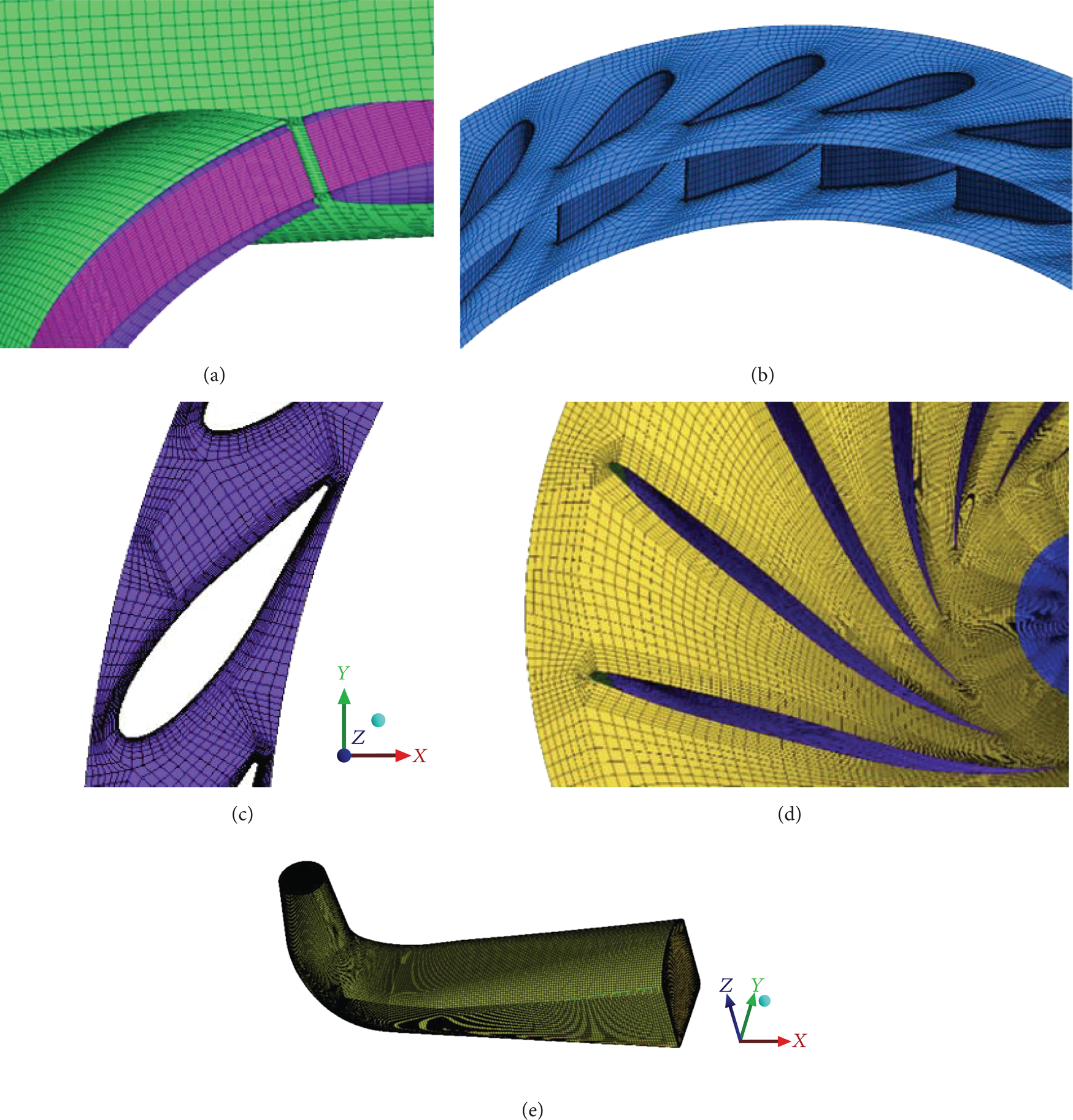
Structured meshes for 5 different parts of the Francis turbine: (a) spirical casing, (b) stay vanes, (c) guide vanes, (d) runner, and (e) draft tube.

2.2. Numerical Method

This study utilized LES method with a certain two-phase cavitating model which is based on the vaporizing-condensing process to simulate the cavitating flow in the Francis turbine. With the assumption of an incompressible working fluid, the governing equations are summarized as follows.

The LES method resolves large scale of the flow field solution, while models resolve small scale of solution which is filtered by filtering operating function. Thus the filtered governing equations are as follows.

Continuity equation:

\frac{\partial {\bar{u}}_{i}}{\partial x_{i}} = 0

(1)

momentum equation:

\frac{\partial {\bar{u}}_{i}}{\partial t} + \frac{\partial ({\bar{u}}_{i} {\bar{u}}_{j})}{\partial x_{j}} = - \frac{1}{ρ} \frac{\partial \bar{p}}{\partial x_{i}} + ν \frac{\partial}{\partial x_{j}} [(\frac{\partial {\bar{u}}_{i}}{\partial x_{j}} + \frac{\partial {\bar{u}}_{j}}{\partial x_{i}})] + \frac{\partial τ_{i j}}{\partial x_{j}},

(2)

where τ_ij is the so-called sub-grid-scale (SGS) stress which will be modeled to enclose the above equations and the parameters with a bar represent the resolvable scale part. In the current investigation, Smagorinsky model is employed to compute τ_ij.

For the cavitation model, the process of vaporizing and condensing can be described by

\begin{matrix} \frac{\partial (ρ_{v} α_{v})}{\partial t} + \frac{\partial}{\partial x_{j}} (ρ_{v} {\bar{u}}_{j} α_{v}) = {\dot{m}}^{+} - {\dot{m}}^{-}, \\ \frac{\partial (ρ_{l} α_{l})}{\partial t} + \frac{\partial}{\partial x_{j}} (ρ_{l} {\bar{u}}_{j} α_{l}) = - ({\dot{m}}^{+} - {\dot{m}}^{-}), \end{matrix}

(3)

where ρ is the density, α is the volume fraction for each phase (subscripts v and l represent vapor phase and liquid phase, resp.), and ${\dot{m}}^{+}$ and ${\dot{m}}^{-}$ are the mass exchange rates caused by vaporizing and condensing processes, respectively.

Thus, the total exchange of mass flow between the vapor and liquid for a unit volume is

\dot{m} = {\dot{m}}^{+} - {\dot{m}}^{-} = N_{B} \frac{d (ρ_{v} 4 π R_{B}^{3} / 3)}{d t} = 4 π N_{B} ρ_{v} R_{B}^{2} \frac{d R_{B}}{d t}

(4)

therein, N_B is the number of cavity bubbles, and R_B is the typical radius of cavity bubble.

Employing the Zwart-Gerber-Belamri (ZGB) cavitation model, the source terms for evaporation and condensation are expressed as follows:

\begin{matrix} {\dot{m}}^{+} = C_{e} \frac{3 α_{nuc} ρ_{v} (1 - α_{v})}{R_{B}} \sqrt{\frac{2}{3} \frac{\max (p_{v} - p, 0)}{ρ_{l}}}, \\ {\dot{m}}^{-} = C_{c} \frac{3 ρ_{v} α_{v}}{R_{B}} \sqrt{\frac{2}{3} \frac{\max (p - p_{v}, 0)}{ρ_{l}},} \end{matrix}

(5)

where α_nuc is the volume fraction of vapor nucleation point and C_e and C_c are the vaporizing coefficient and condensing coefficient, respectively.

On the numerical settings, the second-order Crank-Nicolson method was adopted for temporal marching. The SIMPLEC scheme was used for pressure-velocity coupling; the second-order upwind scheme for pressure iterations and fourth-order central-difference scheme for momentum were set for spatial discretization. And near the wall zone, the flow was treated by using a standard wall function. The residual criteria were set to 10⁻⁵ and the time steps were given separately according to the flow conditions in order to ensure the runner rotating 1 degree within one time step.

On the boundary conditions, the total pressure was given at the inlet of spiral casing, which was determined by model test result. The static pressure was set at the outlet of draft tube, determined by the cavitation coefficient in the experiment. And the no-slip boundary condition was used at the walls.

3. Results and Discussions

The operating conditions of numerical simulation for flow in the hydroturbine were shown in Table 2, including the points where either channel vortex or vortex ropes can be found in the runner or draft tube and flow features nearest to the best efficiency point (BEP) as well.

Table 2:

Parameters of computational conditions.

Openings ofguide vanes	n₁₁ (r/min)	Q₁₁ (m³/s)	σ

10 mm	54.5	0.2515	0.3408
	59.9	0.2432	0.3403
	64.9	0.2550	0.3403

14 mm	55.0	0.3691	0.3410
	60.1	0.3615	0.3403
	65.4	0.3467	0.3402

18 mm	55.3	0.4471	0.3387
	60.6	0.4378	0.3388
	65.0	0.4266	0.3377

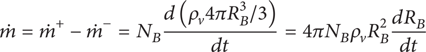
We have performed a series of simulations for different openings of guide vanes, that is, a = 10 mm, 14 mm, and 18 mm (the rated opening of guide vanes). According to these settings, typical cavitating phenomena were captured by changing the unit rotating speed. The operating conditions were listed in Table 2, where n₁₁ was the unit rotating speed as aforementioned, Q₁₁ was the unit flow rate, and σ was the cavitation coefficient. These flow conditions were also clarified in red circles in the synthetical characteristic chart for hydraulic test (Figure 4).

Figure 4:

Synthetical characteristic chart for hydraulic test of Francis hydroturbine model. Therein the points for numerical simulation were marked in red circles.

Firstly, we should validate the calculations under the numerical settings above, and this was confirmed by comparing the external characteristics, that is, the relationship of n₁₁ versus Q₁₁, with the hydraulic model test. Figure 5 quantitatively suggested that the numerical results were consistent with the experiments. In the following, the visualization of the vortex rope and channel vortex was performed, which further verified that the current simulation was reliable and agreed well with the experiments. Then the flow features in the vaneless region were studied, focusing on the pressure oscillation and the evolution of TKE.

Figure 5:

Comparison of external characteristics with experiments for different guide vanes’ openings.

3.1. Flow in the Draft Tube and Runner

To obtain the patterns of cavitating area in the draft tube, the criterion of vapor volume fraction by 10% was used to extract the shape of vortex rope from multiphase calculation results. Figure 6 just displays the helical form of vortex rope at operating condition of a = 14 mm and n₁₁ = 55.0 r/min, showing excellent agreement with former experimental results [35]. The results of other conditions have similar patterns, and all considerably reproduce the patterns in the experiments.

Figure 6:

The patterns of vortex rope by simulation and experiments at condition of a = 14 mm, n₁₁ = 55.0 r/min. For simulation, the cavitation region is defined to be where the volume fraction of vapor is 10%. (a) Two-phase simulation; (b) experimental result.

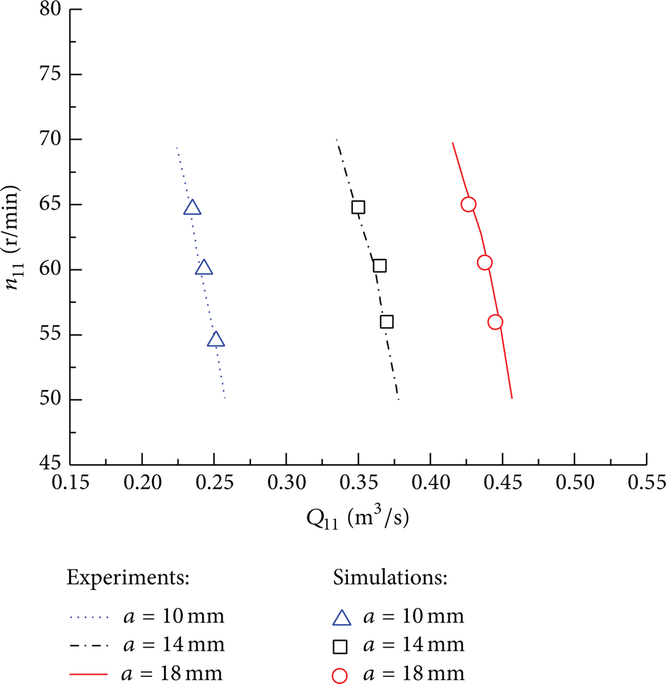
For the channel vortex in the passage between the neighboring blades, we utilized the vorticity criterion to illustrate the features of channel vortices in the runner. This criterion [36] can correctly define the vortex region by giving a threshold value for vorticity measure. It works well in the bulk of channel passage, whilst it may encounter confusion at the near wall region where the strong shear effect exists. However, the vorticity criterion could just precisely capture the patterns of channel vortices. Vorticity denotes the measure of rotation of velocity, and thus the channel vortex induced by secondary flow would fit motions of translating and rotating. Figure 7 shows the channel vortices in the runner distributing along the flow direction based on cavitation model at condition of a = 10 mm, n₁₁ = 59.9 r/min. The threshold for channel vortex illustration is half of the ensemble average value of vorticity magnitude in the runner, that is, 0.5〈|ω|〉. Compared with experiments [35], it is found that the multiphase calculation can well reproduce the cavitating flow in the channel passages. They both present a main stripe of cavitating region along the flow direction with separately isolated secondary cavitating bubbles at the transverse direction, indicating results based on cavitation model can capture most of the features of channel vortices accurately.

Figure 7:

Channel vortex displayed by vorticity criterion at condition of a = 10 mm and n₁₁ = 59.9 r/min. The shape of channel vortex is defined by the isosurface of vorticity magnitude in the runner, and the threshold is 0.5 〈|ω|〉.

3.2. Flow in the Vaneless Area

We now focus on the flow in the gap between guide vanes and the runner; the results for all three different openings of guide vanes will be compared.

3.2.1. Flow Phenomena around Guide Vanes

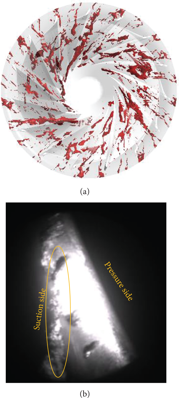
Before the fluid enters the runner, the guide vanes will direct the flow providing a certain contact angle to the moving blades, with minimum loss of energy. We have compared the average flow field for the guide vanes’ opening of 14 mm with the PIV experiments [35], as shown in Figure 8. Both results are derived from 200 samples of instantaneous data at the half-height plane of guide vanes, and the flow conditions keep the same, that is, n₁₁ = 65.4 r/min. It seems that the simulations recover the flow patterns at the regions over and behind the guide vanes, and the velocity at the pressure side is higher than that at the suction side.

Figure 8:

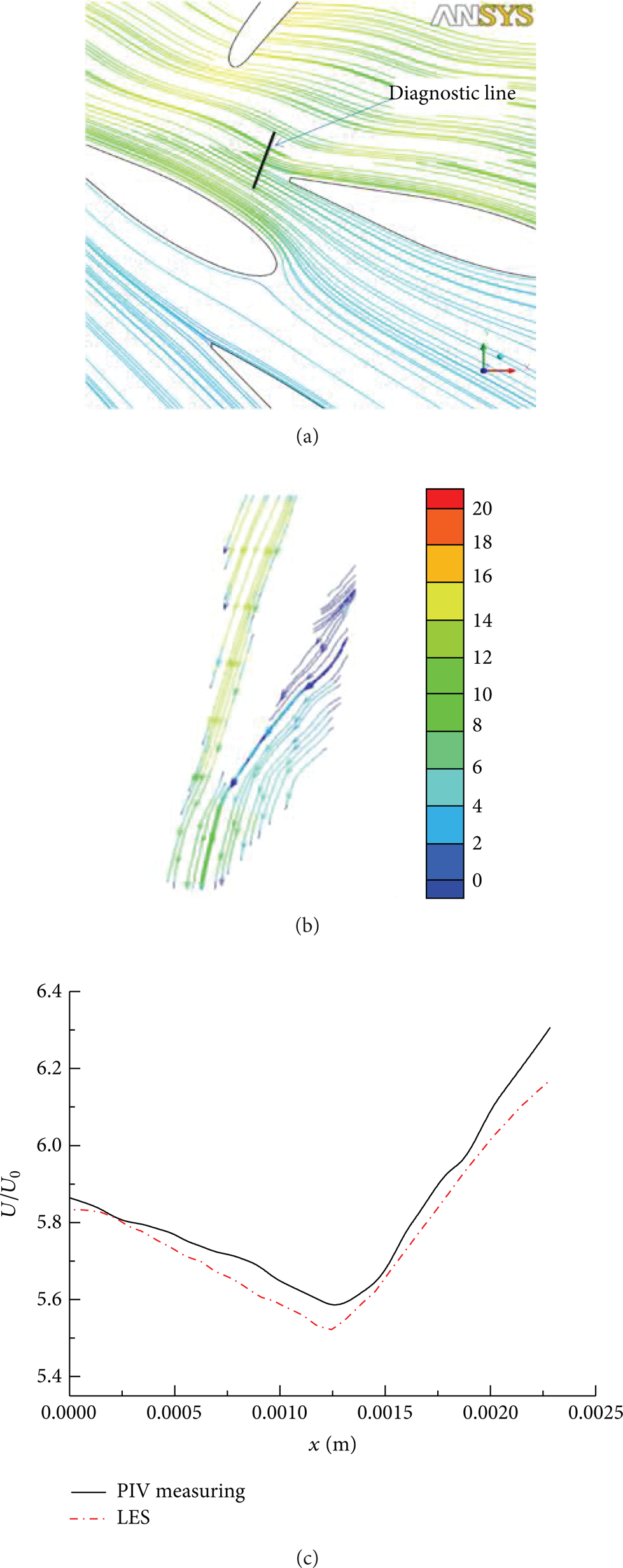
Comparison of vaneless region flow between two-phase flow simulation and experimental result by [35]. The operating condition is a = 14 mm and n₁₁ = 65.4 r/min, and the comparison is conducted on the diagnostic line in the wake region which is marked in black line in (a). (a) Simulation, (b) PIV measuring result, and (c) the nondimensional velocity varying along the diagnostic line.

To quantitatively describe the flow field in the wake region behind the trailing edge of a guide vane, the average dimensionless velocity U/U₀ on the diagnostic line is extracted (Figure 8(c)). Therein, U is the local absolute velocity, and U₀ is superficial velocity at the inlet of spiral casing calculated by the ratio of flow rate and the area of cross-section of casing inlet. The line for test is located at the distance of s/c = 0.2 off the rear of guide vane, whose definition in coordinates (s,n,z) is given in Figure 11, and c is the chord length of guide vane. The results show that the velocity at the wake centerline maintains a minimum, and it grows faster at the pressure side more than suction side. Such difference should be part of reasons of flow irregularity at downstream. However, the trends of velocity distribution remain the same and the simulation agrees well with the experimental measuring.

3.2.2. Pressure Oscillations

The pressure fluctuation in the vaneless region should have a direct relationship with the flow state over the guide vanes. When flow passes through the channels confined by guide vanes, the vanes will convert a part of pressure energy of the fluid at their entrance to the kinetic energy of flow and then direct the fluid onto the runner blades at the angle appropriate to the design. Moreover, fluid from the entrance of guide vanes will accelerate because of their convergent shape of confined channels. Thus the fluid enters the high-speed rotating runners.

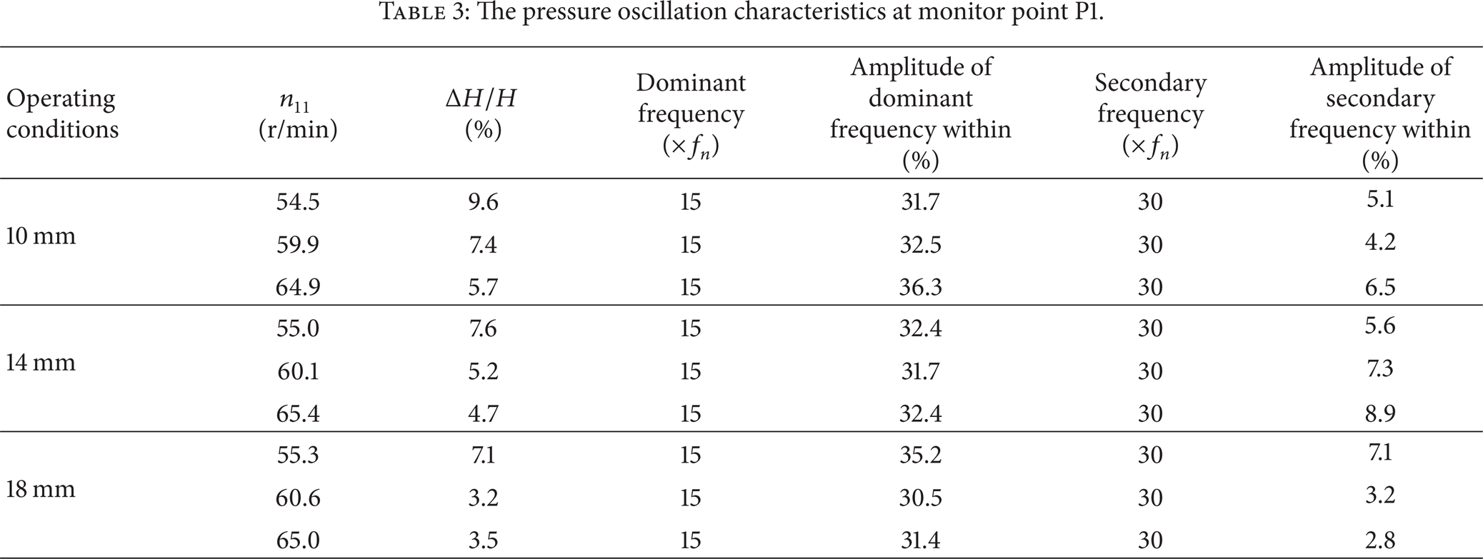
Figure 9 gives the pressure oscillations in the area behind the guide vanes and before the runner. For the guide vanes’ opening of a = 18 mm, the pressure variations for n₁₁ ranging from 55.3 r/min to 65.0 r/min at the monitoring position P1 (Figure 9(a)) in the frequency domain are demonstrated. The details of pressure oscillation characteristics are given in Table 3. The intensity of the pressure oscillations is measured by the parameter of peak-to-peak value ΔH/H, where H is the water head for current operating condition. It reveals that the pressure oscillation augments its amplitude as the opening of vanes turns down if n₁₁ remains unchanged. Meanwhile, off BEP, the magnitude of pressure fluctuation also climbs high when the (unit) rotating speed gets lower. It is worth noting that the magnitude of dominant frequency fluctuations does not change much for all the conditions, whilst that of secondary frequency fluctuations falls off rapidly as the turbine running near to BEP.

Table 3:

The pressure oscillation characteristics at monitor point P1.

Operating conditions	n₁₁ (r/min)	ΔH/H (%)	Dominantfrequency(× f_n)	Amplitude of dominant frequency within (%)	Secondary frequency (× f_n)	Amplitude ofsecondary frequency within (%)

10 mm	54.5	9.6	15	31.7	30	5.1
	59.9	7.4	15	32.5	30	4.2
	64.9	5.7	15	36.3	30	6.5

14 mm	55.0	7.6	15	32.4	30	5.6
	60.1	5.2	15	31.7	30	7.3
	65.4	4.7	15	32.4	30	8.9

18 mm	55.3	7.1	15	35.2	30	7.1
	60.6	3.2	15	30.5	30	3.2
	65.0	3.5	15	31.4	30	2.8

Figure 9:

(a) Locations of monitoring points P1 and P2 and (b) pressure fluctuation features at point P1.

However, to consider the characteristics of oscillation frequencies, the dominant frequencies and secondary frequencies remain the same for all the operating conditions, which are the integral times of blade passing frequency f_n. This is known to be the nature of flow in the turbines.

For monitoring the pressure oscillation, we also extract the results from point P2, which is located at the symmetric position with P1; that is, their geometric positions shift 180 degrees to each other. Figure 10 presents both the fluctuations of pressure and velocity at positions P1 and P2 for a = 18 mm and n₁₁ = 65.0 r/min, and those data are chosen when the flow state approaches stability. Considering the relationship between local pressure and velocity variations, it is shown that they both have a phase difference approaching π/2, with cross-correlation coefficients of 0.45 and 0.48 for P1 and P2, respectively. This would indicate that the fluctuating pressure and velocity are reasonably correlated locally at vaneless region, playing a role of TKE diffusion since the monitoring positions are in the shear wake.

Figure 10:

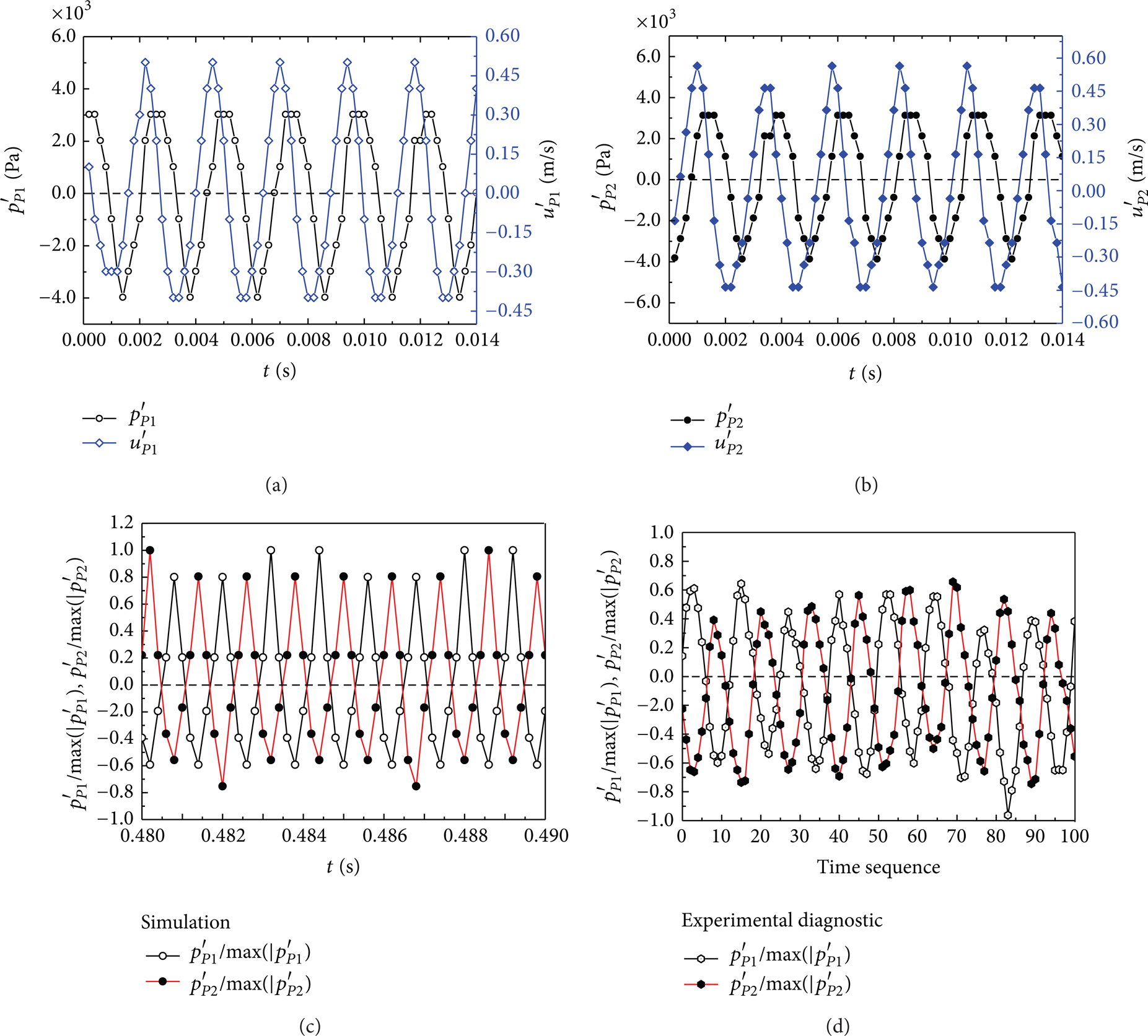
The fluctuations of pressure and velocity at positions P1 and P2 for a = 18 mm and n₁₁ = 65.0 r/min. (a) Pressure and velocity fluctuations at P1, (b) pressure and velocity fluctuations at P2, (c) the nondimensional pressure fluctuations from simulation reduced by the maximum amplitude for P1 and P2, and (d) the experimental measurement of pressure fluctuations for P1 and P2.

Figure 11:

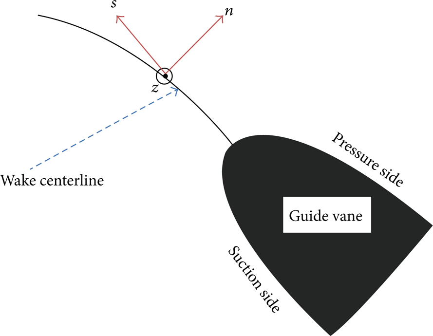
The schematic of curvilinear coordinates (s,n,z).

Moreover, from simultaneous evolution of pressure fluctuations for P1 and P2, they show a clear phase difference of π, and it should stem from the combination of their geometric positions and internal flow features. For comparison, Figure 10(d) exhibits the experimental diagnostics on the pressure oscillations at P1 and P2 points. It reveals the same variations as the simulation presents. Thus it may be deduced that the stresses variations on the runner induced by pressure oscillation are in an odd number of nodal diameter, based on the rotor-stator interaction theory [22].

3.2.3. Features of TKE at Wake Region

Wakes will emerge at the trailing edge of a barrier when the fluid flow is passing through it. As discussed above, the TKE will be rebudgeted at the wake region.

From the equation of TKE,

\frac{\partial k}{\partial t} = - U_{j} \frac{\partial k}{\partial x_{j}} + \frac{\partial}{\partial x_{j}} (- \frac{1}{ρ} 〈 p u_{i}^{'} 〉 δ_{i j} - \frac{1}{2} 〈 q^{2} u_{j}^{'} 〉 + ν \frac{\partial k}{\partial x_{j}}) - 〈 u_{i}^{'} u_{j}^{'} 〉 \frac{\partial U_{i}}{\partial x_{j}} - ν (\frac{\partial u_{i}^{'}}{\partial x_{j}} \frac{\partial u_{i}^{'}}{\partial x_{j}}),

(6)

where k represents the TKE. The pressure diffusion term (which includes the parameter p) represents only the transportation contribution or propagation of pressure variations on TKE distribution, without decaying or generation. It has been proved to be an infinitesimal value which was simply neglected in an axisymmetric jet [37] or cylinder wake [38], and if not, it was measured to be much less than turbulence diffusion effect in a planar wake [39] and low-pressure turbine blade wake [40]. On the other hand, TKE varies along the flow direction, and its production would be responsible for the turbulence intensities in the vicinity of runner inlet. It was revealed that the production and turbulence diffusion terms were the most significant in the TKE balance with convection and dissipation effect. Specifically in engineering situations, the kinetic energy is partly removed from the mean motion and added to the fluctuations, so the production term usually acts to increase the TKE. Therefore, to study the TKE production, we could also attempt to understand the manner of how the TKE sustains the local turbulence level.

In order to understand the mechanism of irregular flow state at the wake region, we try to analyze the evolution of TKE in curvilinear coordinates (s,n,z) based on wake centerline and the trailing edge of guide vane. The schematic of curvilinear coordinates (s,n,z) is shown in Figure 11, where s is on the tangential direction of wake centerline, n is on the perpendicular direction of s, and z is perpendicular to (s,n) plane, that is, parallel with the height of guide vane. Therein, the wake centerline is the very streamline separating the pressure side flow from suction side flow, along which the normal component of velocity is zero.

Therefore, TKE reads as k = 0.5〈u_s^′2 + u_n^′2 + u_z^′2〉 in curvilinear coordinates (s,n,z), where u_s′, u_n′, and u_z′ are the three corresponding fluctuating velocity components. Figure 12 shows the TKE distribution in the wake region and runner for the same (similar) n₁₁ value at different openings of guide vanes. The data are given in the center plane along the streamwise flow direction. At the small opening, TKE peaks at vaneless region, and as the opening grows, TKE gets decreased in the wake and, however, augments at the pressure side of runner inlet. Figure 13 gives another comparison of TKE distribution with varying n₁₁ at a = 4 mm. It illustrates that TKE gets weaker when n₁₁ increases and its distribution becomes laminarly uniform. Moreover, when a and n₁₁ approach the optimal running condition, the maximum value translates to the pressure side of runner blade, and TKE is minimum at the wake region. The TKE peak is shown to be approximately half of that at a = 10 mm. That indicates that the pressure oscillations also reduce as the velocity oscillations get lower.

Figure 12:

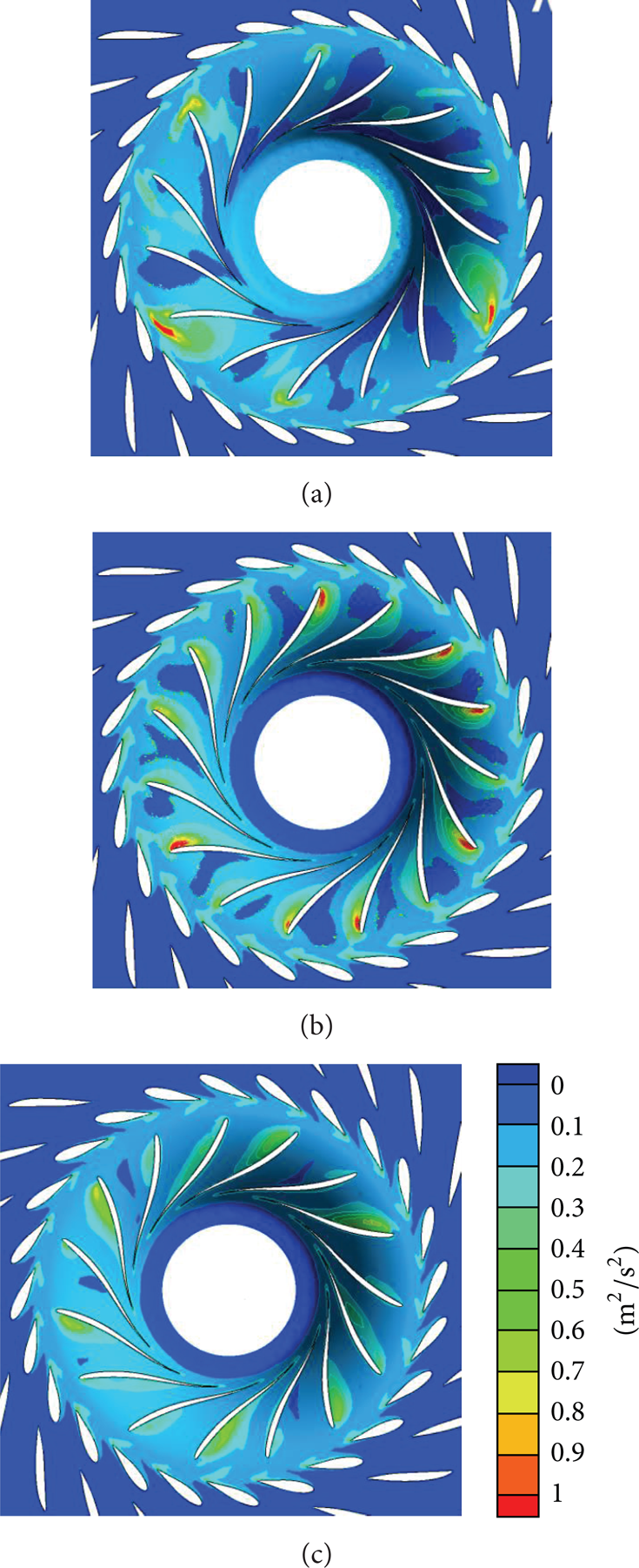
Distribution of turbulent kinetic energy k for different guide vanes’ openings. (a) a = 10 mm, n₁₁ = 54.5 r/min, (b) a = 14 mm, n₁₁ = 55.0 r/min, and (c) a = 18 mm, n₁₁ = 55.3 r/min.

Figure 13:

Distribution of turbulent kinetic energy k for different n₁₁ at a = 14 mm. (a) n₁₁ = 55.0 r/min, (b) n₁₁ = 60.1 r/min, and (c) n₁₁ = 65.4 r/min.

At Figure 14, it shows the three TKE components’ distribution at a = 10 mm and n₁₁ = 54.5 r/min only; the other cases have similar trends for every TKE component's portion in total. They also represent the very different normal Reynolds stress patterns. At this condition, the most of TKE generates at the wake region due to flow contraction, and 〈u_s^′2〉 is by far the largest contributor to the TKE both in the vaneless area and in the runner region, followed by 〈u_n^′2〉 and 〈u_z^′2〉.

Figure 14:

Distribution of TKE components for n₁₁ = 54.5 r/min at a = 10 mm. (a) 〈u_s^′2〉, (b) 〈u_n^′2〉, and (c) 〈u_z^′2〉.

In the following we examined all the TKE production terms in the corresponding Reynolds stress production rate. Katz group has presented an alternative form of TKE equation based on such curvilinear coordinates [32, 33]. Using that, the contributions of several Reynolds stress components to the kinetic energy production can be elucidated in the wake. Thus, we translated the results under the Cartesian coordinates into the expressions under (s,n,z) coordinates. The examining of TKE is performed in the area marked as four blue lines in Figure 15, that is, s/c ranging from 0.1 to 0.4.

Figure 15:

Schematics of region of TKE measuring.

According to previous work [32, 33], the TKE production term 〈u_i′u_j′〉(∂U_i/∂x_j) in (6) can be decomposed into four terms, that is, the normal stresses production term P_n, shear stress production term $P_{t}$ , curvature production term P_w, and three-dimensional production term P_d. The following data are derived from running conditions at n₁₁~60 r/min and a ranging from 10 to 18 mm.

The so-called normal stresses production term P_n reads as

P_{n} = \frac{1}{h} \bar{u_{s}^{' 2}} (\frac{\partial \bar{U_{s}}}{\partial s} + \frac{\bar{U_{n}}}{R}) - \bar{u_{n}^{' 2}} \frac{\partial \bar{U_{n}}}{\partial n},

(7)

where R is the local curvature radius of wake centerline and h = 1 + n/R. The distribution of P_n for various conditions is shown in Figure 16. As the opening grows, P_n becomes lower near to the trailing edge of guide vane but gets larger near to the runner inlet, indicating that the flow carries the fluctuating energy further downstream. For the optimal opening a = 18 mm, P_n shows almost zero along the measuring line s/c = 0.1, and its final peak value at s/c = 0.4 is less than the maximum value for a = 10 mm at s/c = 0.1. From this picture, it is also suggested that the normal Reynolds stress does not contribute to the TKE any more in the vicinity of runner inlet at small opening of guide vanes, since the wake flow may contain vortices there. And in that case, the shear stress production would contribute more TKE.

Figure 16:

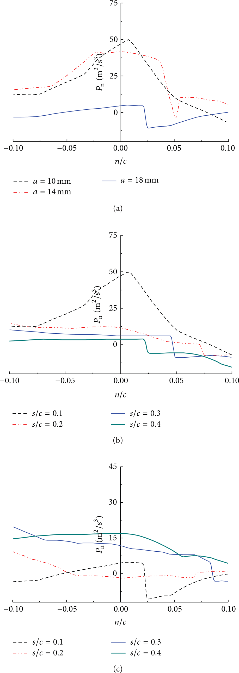
The normal stress production term distribution P_n. (a) For different guide vanes’ openings at s/c = 0.1, (b) for a = 10 mm, and (c) for a = 18 mm.

The shear stress production term P_t reads as

P_{t} = \bar{u_{s}^{'} u_{n}^{'}} (\frac{\partial \bar{U_{s}}}{\partial n} + \frac{1}{h} \frac{\partial \bar{U_{n}}}{\partial s}) .

(8)

This term represents the shear Reynolds stress contribution to the TKE. Figure 17 displays the P_t distribution along the measuring lines for different running conditions. It shows that P_t almost occurs at the pressure side of vanes, where the runner exists. As expected, more P_t contributes to the TKE when the vanes’ opening is small. It is worth noting that the peak value of P_t happens at the very pressure side n/c~0.1 for a = 10 mm, while at the same location for a = 18 mm, the peak value is less than that for 10 mm. The larger the vanes’ opening is, the more the curve shifts right (Figure 17(a)), indicating that large shear stress component occurs near the trailing edge of vanes at small vanes’ opening. However, the maximum P_t turns up around s/c = 0.3 and n/c~0.05 for a = 18 mm, which decreases sharply at downstream, which should be a result of wake evolution induced by vane-runner interaction.

Figure 17:

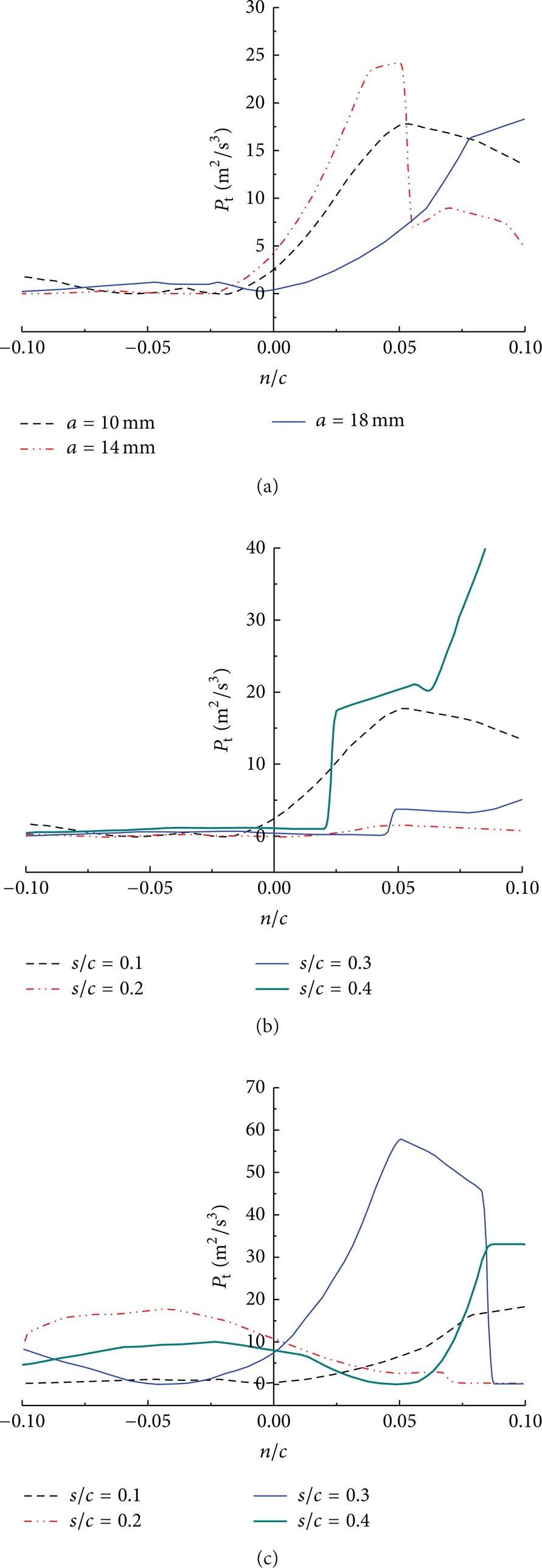
The shear stress production term distribution P_t. (a) For different guide vanes’ openings at s/c = 0.1, (b) for a = 10 mm, and (c) for a = 18 mm.

The curvature production term P_w reads as

P_{w} = \frac{1}{h} \bar{u_{s}^{'} u_{n}^{'}} \frac{\bar{U_{s}}}{R} .

(9)

This term is composed of shear Reynolds stress and the average streamwise velocity gradient at curvature radius. It is a measure of how much TKE is produced towards the curvature center. The distribution of P_w is provided in Figure 18. Comparing with normal stress production term and shear stress production term, this curved effect is one order less than them. Again, at small guide vanes’ opening, P_w at pressure side is larger than that at suction side, and it decreases at flow downstream, indicating that the curved effect on turbulent flow is low. However, for large opening, most of the P_w translates from suction side near trailing edge to pressure side of downstream, which is the interaction zone with runner blades.

Figure 18:

The curvature production term distribution P_w. (a) For different guide vanes’ openings at s/c = 0.1, (b) for a = 10 mm, and (c) for a = 18 mm.

The three-dimensional production term P_d reads as

P_{d} = (\bar{u_{s}^{'} u_{z}^{'}} \frac{\partial \bar{U_{s}}}{\partial z} + \bar{u_{s}^{'} u_{z}^{'}} \frac{\partial \bar{U_{z}}}{\partial s}) + (\frac{1}{h} \bar{u_{s}^{'} u_{z}^{'}} \frac{\partial \bar{U_{z}}}{\partial s} + \bar{u_{n}^{'} u_{z}^{'}} \frac{\partial \bar{U_{z}}}{\partial n} + \bar{u_{z}^{' 2}} \frac{\partial \bar{U_{z}}}{\partial z}) .

(10)

This term contains all the shear stresses with z-direction velocity fluctuations; therefore, it is a measure of TKE generation in three-dimensional flow space. The results of P_d are exhibited in Figure 19 for different vanes’ openings. As the opening decreases, the values get larger, leading to the stronger spatial irregularity of flow. However, for all the openings, the P_d values are less than 1, which are two orders of magnitude lower than P_n and P_t, accounting for the least portion in the total TKE production term. Thus, its influence on the flow stability can be neglected.

Figure 19:

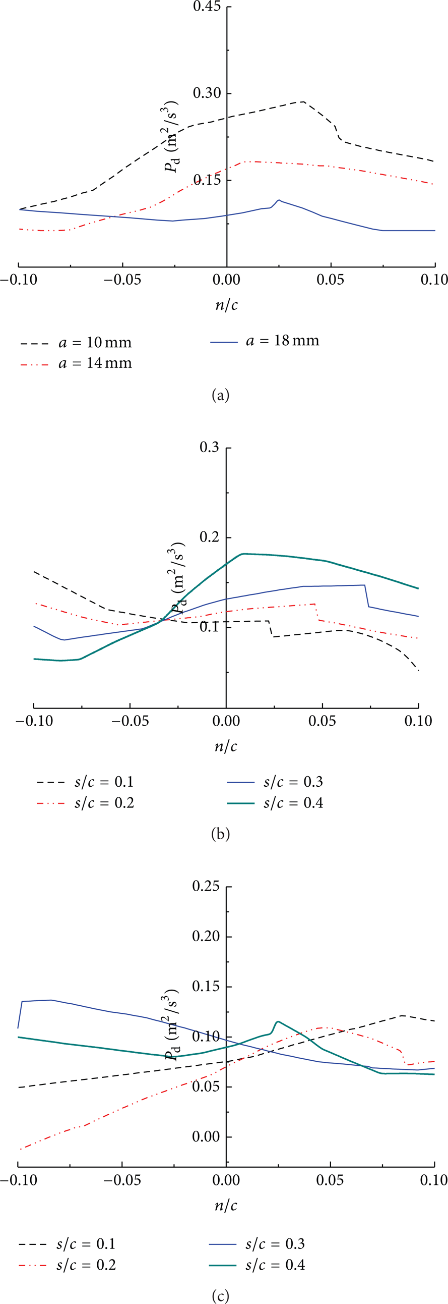
The three-dimensional production term distribution P_d. (a) For different guide vanes’ openings at s/c = 0.1, (b) for a = 10 mm, and (c) for a = 18 mm.

Now, it can be seen that the normal and shear stress production terms impose the most influence on the flow instability in the wake region, followed by the curvature production term, and the three-dimensional production term is usually neglectable.

4. Conclusion

The flow instability with pressure oscillation, pressure-velocity correlation, and turbulent kinetic energy in a large-scale Francis hydroturbine are numerically investigated using LES method. Three sets and total nine runs of simulations are performed, which lie in the low flow-rate conditions. The LES method with two-phase cavitation model could accurately capture the main features of draft tube vortex, channel vortex, fluctuating pressure, and velocities, and the TKE evolution in the wake region after the guide vanes is also analyzed in detail in curvilinear coordinates (s,n,z). The results from pressure oscillation by two monitoring points show that the possible stress variation on the runner induced by fluctuating pressure is in an odd number of nodal diameter.

The main results are concluded as follows.

The magnitude of pressure fluctuations in the wake region grows as the guide vanes’ opening or rotating speed decreases.

The TKE decreases when the guide vanes’ opening turns down, indicating that the turbulence level is falling off. And the TKE distribution will become more laminarly regular in the wake and runner when the vanes’ opening gets large.

The TKE contribution in the vanes’ wake region and runner is mainly from the streamwise velocity component 〈u_s^′2〉, followed by 〈u_n^′2〉 and 〈u_z^′2〉.

Considering the production terms of TKE equation, the normal stress production term and shear stress production term contribute the most to TKE than other production terms.

Conflict of Interests

The authors declare that there is no conflict of interests regarding the publication of this paper.

Footnotes

Acknowledgments

This work is supported by the Foundation for Innovative Research Groups of the National Natural Science Foundation of China under Grant no. 51121004 and National Natural Science Foundation of China under Grant no. 51276046.

References

Dörfler

Sick

, and Coutu

, Flow-Induced Pulsation and Vibration in Hydroelectric Machinery, Springer, London, UK, 2013.

Sick

Michler

Weiss

, and Keck

, “Recent developments in the dynamic analysis of water turbines,” Proceedings of the Institution of Mechanical Engineers A: Journal of Power and Energy, vol. 223, no. 4, pp. 415–427, 2009.

Lambourne

N. C.

and Bryer

D. W.

, “The bursting of leading edge vortices—some observation and discussion of the phenomenon,” Aeronautical Research Council, Report 3282, 1961.

Zhang

R.-K.

Cai

Q.-D.

J.-Z.

Y.-L.

Liu

S.-H.

, and Zhang

, “The physical origin of severe low-frequency pressure fluctuations in giant francis turbines,” Modern Physics Letters B, vol. 19, no. 28–29, pp. 1527–1530, 2005.

Susan-Resiga

T. C.

Muntean

Ciocan

G. D.

, and Nennemann

, “Jet control of the draft tube vortex rope in Francis Turbines at partial discharge,” in Proceedings of the 23rd IAHR Symposium on Hydraulic Machinery and Systems, Yokohama, Japan, 2006.

Susan-Resiga

Ciocan

G. D.

Anton

, and Avellan

, “Analysis of the swirling flow downstream a francis turbine runner,” Journal of Fluids Engineering, Transactions of the ASME, vol. 128, no. 1, pp. 177–189, 2006.

Zhang

Mao

Chen

, and Liu

, “Characteristics and control of the draft-tube flow in part-load Francis turbine,” Journal of Fluids Engineering, Transactions of the ASME, vol. 131, no. 2, 13 pages, 2009.

Ruprecht

Helmrich

Aschenbrenner

, and Scherer

, “Simulation of vortex rope in a turbine draft tube,” in Proceedings of the 21st IAHR Symposium on Hydraulic Machinery and Systems, Lausanne, Switzerland, September 2002.

Kim

S.-W.

and Chen

C.-P.

, “A multiple-time-scale turbulence model based on variable partitioning of the turbulent kinetic energy spectrum,” Numerical Heat Transfer, Part B: Fundamentals, vol. 16, no. 2, pp. 193–211, 1989.

10.

Kirschner

and Ruprecht

, “Velocity measurement with PIV in a straight cone draft tube,” in Proceedings of the 3rd German-Romanian Workshop on Turbomachinery Hydrodynamics, Timişoara, Romania, May 2007.

11.

Kirschner

Ruprecht

, and Göde

, “Experimental investigation of pressure pulsation in a simplified draft tube,” in Proceedings of the 3rd IAHR International Meeting of the Workgroup on Cavitation and Dynamic Problems in Hydraulic Machinery and Systems, Brno, Czech Republic, 2009.

12.

Jošt

and Lipej

, “Numerical prediction of non-cavitating and cavitating vortex rope in a francis turbine draft tube,” Strojniski Vestnik—Journal of Mechanical Engineering, vol. 57, no. 6, pp. 445–456, 2011.

13.

Kuibin

P. A.

Okulov

V. L.

Susan-Resiga

R. F.

, and Muntean

, “Validation of mathematical models for predicting the swirling flow and the vortex rope in a Francis turbine operated at partial discharge,” IOP Conference Series: Earth and Environmental Science, vol. 12, no. 1, Article ID 012051, 2010.

14.

Iliescu

M. S.

Ciocan

G. D.

, and Avellan

, “Analysis of the cavitating draft tube vortex in a francis turbine using particle image velocimetry measurements in two-phase flow,” Journal of Fluids Engineering, vol. 130, no. 2, Article ID 021105, 2008.

15.

Ciocan

G. D.

Iliescu

M. S.

T. C.

Nennemann

, and Avellan

, “Experimental study and numerical simulation of the FLINDT draft tube rotating vortex,” Journal of Fluids Engineering, vol. 129, no. 2, pp. 146–158, 2007.

16.

Liu

S. H.

S. C.

, and Wu

Y. L.

, “Pressure fluctuation prediction of a model kaplan turbine by unsteady turbulent flow simulation,” Journal of Fluids Engineering, vol. 131, no. 10, Article ID 101102, 9 pages, 2009.

17.

Sieverding

C. H.

, “Recent progress in the understanding of basic aspects of secondary flows in turbine blade passages,” Journal of Engineering for Gas Turbines and Power, vol. 107, no. 2, pp. 248–257, 1985.

18.

Kasper

Rose

M. G.

Staudacher

, and Gier

, “A study of unsteady secondary flow in a water flow axial turbine model,” in Proceedings of ASME Turbo Expo 2008: Power for Land, Sea and Air (GT '08), Berlin, Germany, June 2008.

19.

El-Batsh

Hanna

M. B.

, and Sherif

M. F.

, “Experimental and numerical study of the effect of tip clearance on three-dimensional flow field through linear turbine cascade,” in Proceedings of 8th International Congress of Fluid Dynamics & Propulsion (ICFDP '06), Sharm El Sheikh, Egypt, December 2006.

20.

Escaler

Egusquiza

Farhat

Avellan

, and Coussirat

, “Detection of cavitation in hydraulic turbines,” Mechanical Systems and Signal Processing, vol. 20, no. 4, pp. 983–1007, 2006.

21.

Stein

Sick

Doerfler

White

, and Braune

, “Numerical simulation of the cavitating draft tube vortex in a Francis turbine,” in Proceedings of the 23rd IAHR Section Hydraulic Machinery, Equipment, and Cavitation Symposium, Yokohama, Japan, 2006.

22.

Tanaka

, “Vibration behaviour and dynamic stress of runners of very high head reversible pump turbines,” in Proceedings of the 15th IAHR Symposium on Section Hydraulic Machinery, Equipment, and Cavitation, Belgrade, Serbia, 1990.

23.

Ohashi

, “Case study of pump failure due to Rotor-Stator interaction,” International Journal of Rotating Machinery, vol. 1, no. 1, pp. 53–60, 1994.

24.

Fisher

R. K.

Powell

Franke

Seidel

, and Koutnik

, “Contributions to the improved understanding of the dynamic behavior of pump turbines and use thereof in dynamic design,” in Proceedings of the 22nd IAHR Symposium on Hydraulic Machinery and Systems, Stockholm, Sweden, 2004.

25.

Franke

Fisher

Powell

Seidel

, and Koutnik

, “On pressure mode shapes arising from rotor/stator interactions,” Sound and Vibration, vol. 39, no. 3, pp. 14–18, 2005.

26.

Nicolet

Ruchonnet

, and Avellan

, “One-dimensional modeling of rotor stator interaction in Francis pump-turbine,” in Proceedings of the 23rd IAHR Symposium on Hydraulic Machinery and Systems, Yokohama, Japan, 2006.

27.

Hasmatuchi

Roth

Botero

Avellan

, and Farhat

, “High-speed flow visualization in a pump-turbine under off-design operating conditions,” IOP Conference Series: Earth and Environmental Science, vol. 12, no. 1, Article ID 012059, 2010.

28.

Guillaume

Deniau

J. L.

Scolaro

, and Colombet

, “Influence of the rotor-stator interaction on the dynamic stresses of Francis runners,” IOP Conference Series: Earth and Environmental Science, vol. 15, Article ID 052011, 2012.

29.

Yan

Koutnik

Seidel

, and Hübner

, “Compressible simulation of rotor-stator interaction in pump-turbines,” IOP Conference Series: Earth and Environmental Science, vol. 12, Article ID 012008, 2010.

30.

Lais

Liang

Henggeler

Weiss

Escaler

, and Egusquiza

, “Dynamic analysis of Francis runners—experiment and numerical simulation,” in Proceedings of the IAHR 24th Symposium on Hydraulic Machinery and Systems, Foz do Iguassu, Brazil, October 2008.

31.

Keller

and Sallaberger

, “Modern hydraulic design of pump turbines,” in Proceedings of the International Seminar on Hydropower Plants, Vienna, Austria, November 2006.

32.

Miorini

R. L.

, and Katz

, “Measurements of the tip leakage vortex structures and turbulence in the meridional plane of an axial water-jet pump,” Experiments in Fluids, vol. 50, no. 4, pp. 989–1003, 2011.

33.

H.-X.

Tan

Miorini

R. L.

, and Katz

, “Three-dimensional flow structures and associated turbulence in the tip region of a waterjet pump rotor blade,” Experiments in Fluids, vol. 51, no. 6, pp. 1721–1737, 2011.

34.

and Durbin

P. A.

, “Evidence of longitudinal vortices evolved from distorted wakes in a turbine passage,” Journal of Fluid Mechanics, vol. 446, pp. 199–228, 2001.

35.

W. T.

X. B.

F. C.

Wei

X. Z.

Han

W. F.

, and Liu

S. H.

, “Experimental investigation on the characteristics of hydrodynamic stabilities in Francis hydro-turbine models,” Advances in Mechanical Engineering, vol. 2014, Article ID 486821, 13 pages, 2014.

36.

Metcalfe

R. W.

Hussain

A. K. M. F.

Menon

, and Hayakawa

, “Coherent structures in a turbulent mixing layer: a comparison between direct numerical simulations and experiments,” Turbulent Shear Flows 5, pp. 110–123, 1987.

37.

Panchapakesan

N. R.

and Lumley

J. L.

, “Turbulence measurements in axisymmetric jets of air and helium. Part 1: air jet,” Journal of Fluid Mechanics, vol. 246, pp. 197–223, 1993.

38.

Browne

L. W. B.

Antonia

R. A.

, and Shah

D. A.

, “Turbulent energy dissipation in a wake,” Journal of Fluid Mechanics, vol. 179, pp. 307–326, 1987.

39.

Liu

and Thomas

F. O.

, “Measurement of the turbulent kinetic energy budget of a planar wake flow in pressure gradients,” Experiments in Fluids, vol. 37, no. 4, pp. 469–482, 2004.

40.

Sideridis

Yakinthos

, and Goulas

, “Turbulent kinetic energy balance measurements in the wake of a low-pressure turbine blade,” International Journal of Heat and Fluid Flow, vol. 32, no. 1, pp. 212–225, 2011.

On the Flow Instabilities and Turbulent Kinetic Energy of Large-Scale Francis Hydroturbine Model at Low Flow Rate Conditions

Abstract

1. Introduction

2. Numerical Simulation Procedures and Validation

2.1. Turbine Structure and the Mesh

2.2. Numerical Method

3. Results and Discussions

3.1. Flow in the Draft Tube and Runner

3.2. Flow in the Vaneless Area

3.2.1. Flow Phenomena around Guide Vanes

3.2.2. Pressure Oscillations

3.2.3. Features of TKE at Wake Region

4. Conclusion

Conflict of Interests

Footnotes

Acknowledgments

References