Sage Journals: Discover world-class research

Abstract

We aim to cover a grid fully by deploying the necessary wireless sensors while maintaining connectivity between the deployed sensors and a base station (the sink). The problem is NP-Complete as it can be reduced to a 2-dimensional critical coverage problem, which is an NP-Complete problem. We develop a branch and bound (B&B) algorithm to solve the problem optimally. We verify by computational experiments that the proposed B&B algorithm is more efficient, in terms of computation time, than the integer linear programming model developed by Rebai et al. (2013), for the same problem.

1. Introduction

The emerging wireless sensor networks (WSNs) technology provides an inexpensive and powerful means to monitor physical environments. WSNs are dense but low cost networks, which are formed by wireless nodes that sense certain phenomena in the area of interest and report their observations to a base station for further analysis [1]. WSNs are used in many applications such as environmental monitoring [2], emergency navigation [3], and smart spaces and industrial diagnostics [4, 5].

In a WSN, the sensor deployment is a critical issue because it may affect many facets of the network operations, including power management, routing, quality of service, and detection capability. In general, the sensor deployment is achieved either in a deterministic way or in a random way. Deterministic deployments are used in missions where the deployment area is physically accessible (urban monitoring, target tracking, etc.). On the other hand, random deployments are usually used when the mission deployment area is physically unreachable (seismic zones, volcanoes, etc.) [6].

It is worth noting that good sensor deployment may bring great benefits such as better network management and energy and cost savings, particularly when the sensor price is high. Nevertheless, the sensor placement has to be carried out so that coverage and connectivity are the most important considerations. In fact, while coverage is a metric that measures the surveillance quality provided by a WSN, connectivity offers a means for sensors to report their data to the sink [7].

In the WSN literature, two types of coverage problems are investigated: area coverage and target or point coverage. In the area coverage problem, the deployed sensors have to monitor a given area, whereas, in the target coverage problem, only a set of specific points (or targets) are monitored by the deployed sensors.

Both area coverage and target coverage problems can be divided in the 1-coverage problem or the k -coverage problem. In the latter, each target or point in the sensing area needs to be covered by at least k different working sensors. However, in the 1-coverage problem, each target or point in the sensing field has to be covered by at least one active sensor. Sometimes, the network coverage issue is closely related to the network's energy consumption [8–11]. In our proposal, we do not consider the energy constraint, since we assume that each sensor can be powered by an energy source (this is true in many cases, like fire detection sensors deployed in a large building). We note that the sensor devices may be characterized by a communication range. In such a case, a WSN is considered active if each sensor device finds a path (i.e., a set of connected sensors) towards the sink.

Our general observation regarding previous works on the total coverage problem with connectivity constraint indicates few resolution approaches based on exact optimization methods. In this contribution, we propose a branch and bound algorithm to determine the optimal placement of networked sensors allowing total sensing area coverage such that each sensor device can find a connection path (i.e., a set of connected sensors) which reaches the sink. The rest of the paper is organized as follows. Section 2 briefly discusses related works in the field. Section 3 describes our network model. Section 4 presents a lower bound for the problem. Section 5 describes the B&B algorithm. Section 6 provides simulation results to demonstrate the performance of our proposed work, and finally we conclude the paper and introduce our future work in Section 7.

2. Related Works

The area coverage problem has been thoroughly studied in the last few years. Ke et al. [12] have proved that the problem of fully covering critical grids using a minimum number of sensors (known also as critical grid coverage problem) is NP-Complete. In [13], Chakrabarty et al. propose a linear model to minimize the cost of sensor deployment in a three-dimensional sensing field, while keeping a complete coverage area. In their study, the authors consider two types of sensors with different costs. The authors also assume that each point in the grid has to be covered by at least k sensors. Andersen and Tirthapura [14] consider the total coverage in 3-dimensional area as a set-cover problem with multiplicity k. Another approach, based on the copy of a regular polyhedron with a small volumetric coefficient, was presented by Alam and Haas [15] for the same problem.

A variety of algorithms and protocols achieving total coverage and connectivity have been proposed in the literature. In [16], Shakkottai et al. presented necessary and sufficient conditions for 1-covered, 1-connected sensor grid network. In addition, the authors developed a variety of methods to maintain connectivity and coverage in large WSNs. In [4], Bai et al. proposed an optimal deployment strategy to achieve both full coverage and 2-connectivity regardless of the relationship between the communication and sensing radii of sensors. Also, they established the efficiency of some regular patterns of deployment, thus enabling better decision making. Liu et al. [17] presented a joint scheduling scheme based on a randomized algorithm for providing statistical sensing coverage and guaranteed network connectivity. The authors in [18] proved that if the original network is connected and the chosen active nodes can cover the same region as all the original nodes, then the network formed by the active nodes is connected when the communication range is at least twice the sensing range.

Zhao and Gurusamy [19] developed a greedy algorithm that addressed both sensing coverage and network connectivity and proposed an approach to schedule the active time of sensors such that active sensors can cover all the targets and can be connected to the sink by direct links or by multihop routes traversing through only active sensors. However, the algorithm can only handle the coverage of discrete points. In [20], Gupta et al. introduced the notion of a connected sensor cover, which is defined as the nodes set that can fully cover the queried area and which constitutes a connected communication graph at the same time. In the same work, the authors proved that the computation of the smallest connected sensor cover is NP-hard, and they developed distributed and centralized approximated methods to solve it, providing the performance bounds as well. The authors in [21] generalized the connected coverage problem to the connected k -coverage problem. However, the algorithms in [20, 21] require each individual sensor to be aware of its precise placement to check its local coverage redundancy. In some particular scenarios, it is difficult or infeasible to obtain the precise location information of sensors. Finally, Rebai et al. [22] proposed two integer linear programming models for the problem of total grid coverage. One of the models considers only the total coverage constraint. The other model ensures both the constraint of connectivity between the sensors and the total grid coverage constraint. In their work, the authors do not consider the energy constraint. A review of other existing works on the area coverage problem may be found in [23, 24].

3. Problem Description

The treated problem consists of fully covering a 2-dimensional sensing area, using a minimum number of sensors while maintaining the connectivity between the sensors and the sink. We suppose that the sensing field may be represented by a grid having $M \times N$ (width × length) units of measure. The grid is digitized into $M \times N$ points and the distance between each two adjacent points is equal to 1 measurement unit. A sensor device, placed at the $(i, j)$ grid position, is characterized by a sensing range noted $R_{cov}$ and a communication range noted $R_{com}$ . The sensor must accomplish two main tasks: covering each position $(k, t)$ in the grid verifying $(i - k)^{2} + (j - t)^{2} \leq R_{cov}^{2}$ and communicating the collected information to a next sensor along a path and so on until the information reaches the sink located at position $(l, w)$ . A sensor placed at the $(k, t)$ position can communicate the collected data to another sensor located at the $(p, q)$ position if and only if

\begin{matrix} {(p - k)}^{2} + {(q - t)}^{2} \leq R_{com}^{2} . \end{matrix}

(1)

Figure 1 represents the main characteristics of the problem with a grid of

9 \times 9

R_{cov} = 2

, and

R_{com} = 3

Figure 1

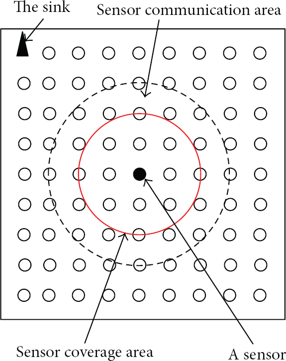
WSN characteristics.

In this study, we assume that $R_{cov} = R_{com} = R$ . Nevertheless, the developed method could be easily extended to the case of $R_{cov} \neq R_{com}$ .

Since our problem has already been treated, the results of the developed B&B algorithm will be compared, in Section 6, to the results of the integer linear programming model proposed by Rebai et al. [22].

4. Lower Bound

The main idea of the developed lower bound is to decompose the grid into small contiguous regular grids. Each small grid is characterized by a length $m \leq M$ and a width $n \leq N$ (M and N are the length and the width of the sensing area or the grid, resp.). By solving the problem of the total small grids coverage so that the connectivity constraint inside each small grid is achieved and the distance between each two sensors in the sensing area (the grid) is greater than or equal to the sensing range R, we obtain a lower bound for the problem.

4.1. Definitions

(1)

Let S be the number of the contiguous regular small grids in the sensing area $M \times N$ .

(2)

Let us consider P as the problem of total grid coverage with connectivity constraint (our treated problem).

(3)

Let us define $B_{i}$ as the subproblem of the total small grid i coverage with connectivity constraint inside the small grid i such that the distance between each two sensors in the sensing area (the grid) is greater than or equal to the sensing range R.

(4)

Let us consider $P_{1}$ as the problem of the total small grids coverage.

4.2. Proposition

If $γ_{i}$ is the optimal solution of the subproblem $B_{i}$ , therefore $δ = \sum_{i = 1}^{S} γ_{i}$ is a lower bound for the problem $P_{1}$ . Consequently, δ is a lower bound for the problem P.

Proof.

When we have a grid with a length M and a width N, we can decompose it in different ways into small contiguous regular grids. All the small grids of $P_{1}$ constitute one part of the grid of P. Hence, a lower bound of $P_{1}$ is also a lower bound of P. When we solve $P_{1}$ , by solving optimally at each iteration $i (i = 1 \dots S)$ the subproblem $B_{i} (i = 1 \dots S)$ , there are two main scenarios that may happen. In the first scenario, connectivity between the small grids is achieved. In such a scenario, δ is an optimal solution if the total grid coverage constraint is achieved. In fact, the total coverage constraint and the connectivity inside and outside the small grids constraint are achieved. Moreover, the change of one sensor position in a small grid leads to the loss of either the coverage constraint in the sensing area (the grid) or the connectivity constraint. Hence, δ is an optimal solution. If the total grid coverage constraint is not reached, δ remains a lower bound since the connectivity between the deployed sensors is reached while the total coverage constraint is not achieved. In the second scenario, the connectivity between the small grids is not achieved. In a such scenario, δ is a lower bound for the problem because the connectivity constraint is automatically relaxed while the distance separating two sensors is greater than or equal to the sensing range R.

Figure 2 illustrates the lower bound idea in the problem with $M = 10$ , $N = 10$ , and $R = 2$ . Figure 2(a) shows the sensing area (the grid) decomposed into 4 regular small grids which means that $S = 4$ . The width and the length of one regular small grid are $n = m = 5$ . Figures 2(b), 2(c), 2(d), and 2(e) represent the process to follow in order to obtain the lower bound value. In Figure 2(b), just $B_{1}$ is solved optimally. In Figure 2(c), $B_{2}$ is solved considering the optimal solution of $B_{1}$ . In Figure 2(d), $B_{3}$ is solved considering the optimal solutions of $B_{1}$ and $B_{2}$ . Finally, in Figure 2(e), $B_{4}$ is solved considering the optimal solutions of $B_{1}$ , $B_{2}$ , and $B_{3}$ . Figure 2(e) shows that $γ_{i} = 4$ which implies that $δ = \sum_{i = 1}^{S} γ_{i} = 16$ . In Figure 2(e), we observe that the total coverage constraint is satisfied while the connectivity constraint is not achieved. Moreover, the change of one sensor position leads to the loss of either the total coverage constraint or the connectivity constraint in the small grid. We note that the total coverage constraint may not be satisfied in some cases. For example, if we consider a grid with a length of 13 measurement units and a width of 12 measurement units, then the total coverage constraint is not satisfied using this lower bound decomposition. However, the delivered solution remains a lower bound for the problem. Note that in our experimental tests each regular small grid has a length $m = ⌈ 5 \cdot R ⌉ / 2$ and a width $n = ⌈ 5 \cdot R ⌉ / 2$ . The optimal solution of each subproblem $B_{i}$ , determined by our decomposition method, is equal to 4 (i.e., $γ_{i} = 4$ ) for $R \geq 2$ . In addition, we can find 4 sensor positions which reach the total small grid coverage. However, connectivity between two contiguous small grids is never reached.

Figure 2

Lower bound procedure.

5. Branch and Bound Algorithm (B&B)

The proposed B&B algorithm aims to determine a connected graph by choosing a limited number of arcs between some connected sensors nodes. Hence, the complexity of the algorithm is $O (2^{(M \times N)})$ . In the remainder of this section, the main elements of the B&B algorithm are given.

5.1. The Initialization

The initial solution of the B&B algorithm is determined as follows. First, the farthest sensor position from the (1,1) grid position, which differs from the sink position and can cover the (1,1) grid position, is chosen. After that, the set, named F, of the all nonselected positions which are different from the sink position and can communicate with the first selected sensor position is determined. Then, the sensor position, which covers the maximum of the uncovered grid points, is selected from the set F. Finally, the last two steps applied to all the selected sensor positions are repeated until a complete solution with $N b$ sensor positions is obtained. Algorithm 1 summarizes the B&B initial solution procedure.

Algorithm 1: The upper bound.

$W = ϕ$ : the set of selected sensor positions.

F: the set of nonselected grid positions which communicate with the positions

of W Select a sensor position (i, j) which covers the (1, 1) position.

$W = W \cup (i, j)$

(1) While (the grid is not fully covered)

Determine F.

Select the position ( $s, t$ ) in F which covers the maximum of uncovered points

$W = W \cup (s, t)$

End while

Nb = $| W |$

5.2. The Branching Scheme

A node at level k of the search tree is defined by the fixed partial solution positions and the node's remaining positions. These latter ones are obtained by the node partial solution border and represent the nodes of the level $k + 1$ of the search tree. In fact, the node partial solution border is the subset, named S, of the covered ( $i, j$ ) (for all $i = 1 \dots M$ , for all $j = 1 \dots N$ ) grid positions having in their neighborhood at least one uncovered grid position from the following set $B = {(Max {i - 1,1}, Max {j - 1,1})$ ; $(Max {i - 1,1}, j); (Max {i - 1,1}, Min {j + 1, N})$ ; $(i, Max {j - 1,1}); (i, Min {j + 1, N}); (Min {i + 1, M}$ , $Max {j - 1,1}); (Min {i + 1, M}, j)$ ; $(Min {i + 1, M}, Min {j + 1, N})}$ .

Figure 3, represents the partial solution border of the node with the partial solution (2,2); (2,4); (3,1); (3,3); (5,1).

Figure 3

The partial solution border $(R = 2)$ .

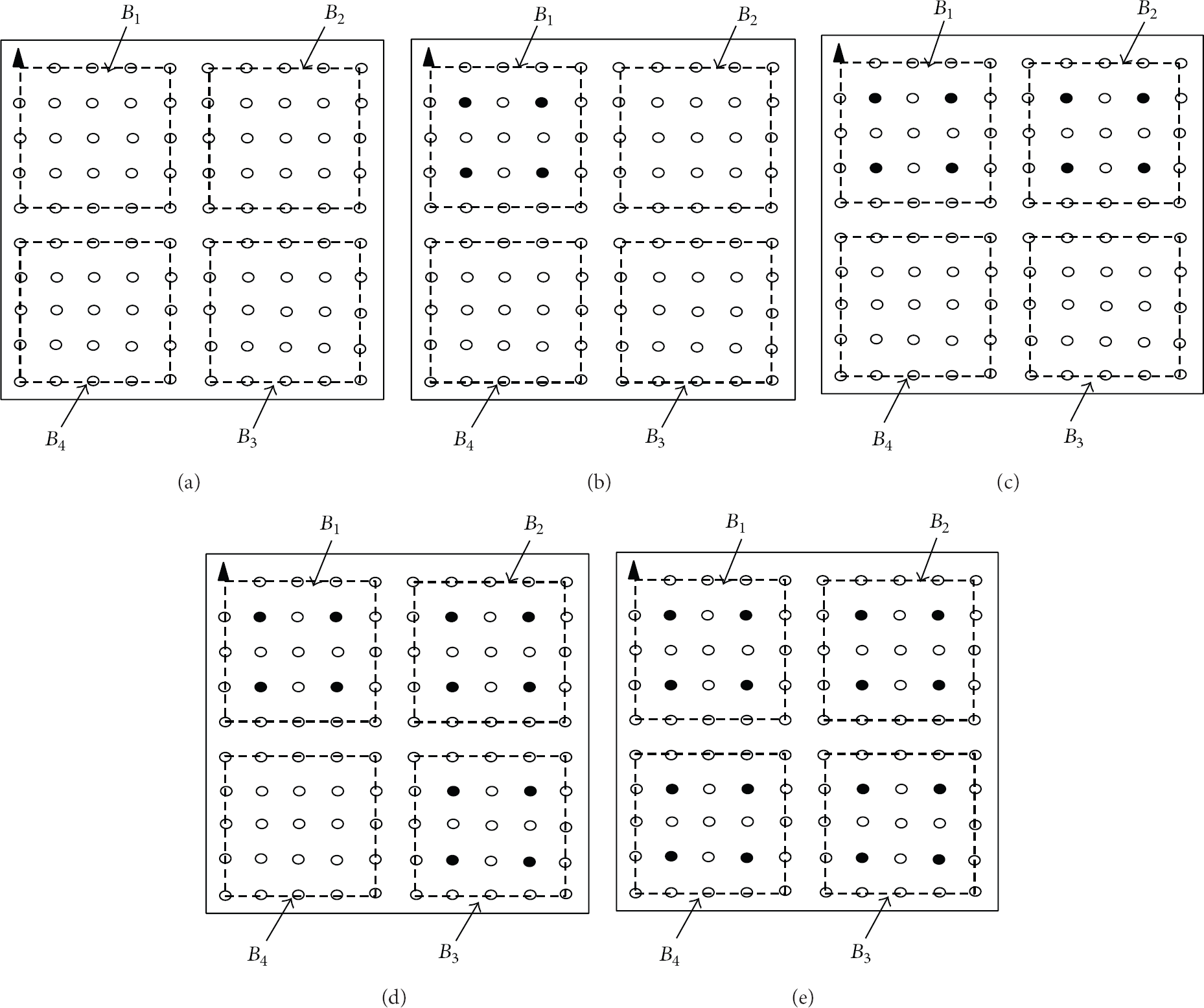
The branching scheme is achieved as follows: we first define the partial solution border of the first level by determining all the $(i, j)$ positions verifying $(l - i)^{2} + (w - j)^{2} \leq R^{2}$ where $(l, w)$ corresponds to the sink position. After that, the separation on the last node of the first level is achieved by adding to the node its remaining sensor positions determined by the node partial solution border S. Then, we repeat, in the second level, the separation on the last node and so on until a complete solution which verifies the total coverage constraint is obtained. This branching schema is called depth first separating strategy. Figure 4 shows the branching procedure on a grid with a length $M = 5$ , a width $N = 5$ , an $R = 2$ , and a sink position $(l, w) = (1,1)$ .

Figure 4

The branching scheme on a grid.

In Figure 4, the light-filled sensor positions in (a), (b), and (c) grids represent the partial solution border positions of the first, the second, and the third levels of the search tree, respectively. In the first grid of Figure 4 (i.e., grid (a)), each one of the $(i, j)$ light-filled positions has at least one uncovered position from the set B. The partial solution border of the first level, which defines the first level nodes, is $S = {(1,2); (1,3); (2,1); (3,1); (2,2)}$ . Since the (2,2) sensor position is the last position in the first level, we separate that node (i.e., (2,2)) by determining, firstly, all the grid positions which can be covered by the (2,2) sensor position and then by defining, in a second step, the partial solution border of the second level $S = {(3,1); (3,2); (4,2); (3,3); (2,3); (1,3); (2,4)}$ which represents the second level nodes. Since the (2,4) sensor position is the last sensor position in the second level, we separate that position by determining all the grid positions which are covered by the (2,2); (2,4) sensor positions and defining the partial solution border of the third level $S = {(3,1); (3,2); (4,2); (3,3); (3,4); (4,4); (3,5)}$ which represents the third level nodes. This procedure is repeated until the total coverage constraint is achieved. Figure 5 represents the branching scheme of the example below using a search tree.

Figure 5

The branching scheme using the search tree.

To enhance the performance of the B&B algorithm, two properties are developed allowing more elimination of fathomed nodes in the search tree.

5.2.1. Definitions

(1)

Let $S_{k}^{i}$ be set of the partial solution border positions of the node i at level k of the search tree (i.e., $S_{k}^{i}$ is the remaining sensor positions of the node i at level k).

(2)

Let us consider $P_{k}^{i}$ as the partial solution positions set of the node i at level k of the search tree.

(3)

Let us consider $(x_{k}^{i}, y_{k}^{i})$ as the last position in $P_{k}^{i}$ .

5.2.2. Property 1

At level k of the search tree, if $(x_{k}^{i}, y_{k}^{i}) \in S_{k}^{j}$ and $(x_{k}^{j}, y_{k}^{j}) \in S_{k}^{i}$ , then the branching scheme contains double solutions. Consequently, we can remove $(x_{k}^{i}, y_{k}^{i})$ from $S_{k}^{j}$ or $(x_{k}^{j}, y_{k}^{j})$ from $S_{k}^{i}$ .

Proof.

At level k of the search tree $P_{k}^{i} - {(x_{k}^{i}, y_{k}^{i})} = P_{k}^{j} - {(x_{k}^{j}, y_{k}^{j})}$ . If $(x_{k}^{i}, y_{k}^{i}) \in S_{k}^{j}$ and $(x_{k}^{j}, y_{k}^{j}) \in S_{k}^{i}$ , we will necessarily find the two partial solutions $P_{k + 1}^{i} = P_{k}^{i} \cup {(x_{k}^{j}, y_{k}^{j})}$ and $P_{k + 1}^{j} = P_{k}^{j} \cup {(x_{k}^{i}, y_{k}^{i})}$ at level $k + 1$ of the search tree which are equal partial solutions. Hence, we can remove one of double solutions from the level k by removing the last fixed position of the node j from the remaining positions of the node i or the last fixed position of the node i from the remaining positions of the node j at level k.

In the example in Figure 4, if we examine the node (3,1) in the second level (L2), then we observe that the partial solution in this node, determined by the fixed sensor positions, is (2,2); (3,1). The separation on the node (3,1) of level 1 (L1) will provide in level 2 (L2) the following partial solution border positions: $S = {(2,1); (2,2); (3,3); (4,1)}$ . We observe in level 2 (L2) a partial solution equal to (3,1); (2,2) which is equal to the partial solution (3,1); (2,2) already treated. Hence, the elimination of the (2,2) sensor position from the remaining position of the node (3,1) in the first level of the search tree will improve the performance of the B&B algorithm in terms of fathomed nodes and computation time.

5.2.3. Property 2

Let $(n, m)$ denote a sensor position which verifies that $(m, n) \in S_{k}^{i}$ and $(m, n) \in S_{k}^{j}$ such that $(x_{k}^{i} - x_{k}^{j})^{2} + (y_{k}^{i} - y_{k}^{j})^{2} > R^{2}$ ; then $(n, m)$ must be removed from $S_{k}^{j}$ or $S_{k}^{i}$ .

Proof.

Consider that $(m, n) \in S_{k}^{i}$ means that $(x_{k}^{i} - m)^{2} + (y_{k}^{i} - n)^{2} \leq R^{2}$ and $(m, n) \in S_{k}^{j}$ means $(x_{k}^{j} - m)^{2} + (y_{k}^{j} - n)^{2} \leq R^{2}$ . If we keep $(n, m)$ in the two remaining sensor positions of the nodes i and j at level k of the search tree, then, in level $k + 1$ , $(n, m)$ will be a sensor position of the partial solution of the node i and a sensor position of the partial solution of the node j while $(x_{k}^{j}, y_{k}^{j})$ will be a remaining sensor position of the node i and $(x_{k}^{i}, y_{k}^{i})$ will be a remaining sensor position of the node j since $(x_{k}^{i} - x_{k}^{j})^{2} + (y_{k}^{i} - y_{k}^{j})^{2} > R^{2}$ , $(x_{k}^{i} - m)^{2} + (y_{k}^{i} - n)^{2} \leq R^{2}$ , and $(x_{k}^{j} - m)^{2} + (y_{k}^{j} - n)^{2} \leq R^{2}$ . At level $k + 2$ of the search tree we will inevitably find the two partial solutions $P_{k + 2}^{i} = P_{k + 1}^{i} \cup {(x_{k}^{j}, y_{k}^{j})}$ and $P_{k + 2}^{j} = P_{k + 1}^{j} \cup {(x_{k}^{i}, y_{k}^{i})}$ which are equal partial solutions. Hence, the elimination of the $(n, m)$ position from $S_{k}^{i}$ or $S_{k}^{j}$ will avoid the onset of a double solution in the search tree.

5.3. The Bounding Procedure

In the bounding step, a lower bound solution of value ${Lb}_{k}$ has to be computed on the remaining uncovered grid positions. In the proposed B&B algorithm, the lower bound described in Section 4 is used. The bounding procedure is achieved as follows: firstly, the number of the regular small grids is determined and the borders of each small grid are defined on the grid. In the second step, the lower bound sensor positions are plotted by placing, in each small grid, the four positions which ensure the total small grid coverage and the connectivity inside the small grid. In the third step, the partial solution positions (with number α) are plotted on the grid. Then, the lower bound sensor positions, of number θ, which communicate with the partial solution sensor positions are deduced from the lower bound value (i.e., δ). Finally, we computed that ${Lb}_{k} = δ - θ$ . The ${Lb}_{k} + α$ value is compared to the current upper bound value. If the latter is greater than the ${Lb}_{k}$ value, we add to the node its remaining positions as described in the branching scheme subsection. In the contrary case, we eliminate the separation on that node.

6. Computational Experiments

An instance for the total sensing field coverage problem with connectivity constraint is generated as follows: we first define the width M and the length N of the sensing field that are, respectively, in the ${7,10,13,15}$ and ${7,10,13,15}$ sets. The sensor sensing range R is, subsequently, defined from the following set: ${2,3, 4,5}$ . Finally, 7 possible positions for the sink placement are tested. The first 5 positions are (1,1), $(1, N)$ , $(M, 1)$ , $(M, N)$ , and $(M / 2, N / 2)$ . The two remaining positions are randomly chosen from $[2, M - 1]$ and $[2, N - 1]$ uniform intervals. We note that this method of instances generation is the same method presented in Rebai et al. since the results of the integer linear formulation proposed by the latter authors are compared to the results of our developed exact method.

The B&B algorithm is coded in the C language and implemented on an Intel core i 7-3720QM CPU 2.60 GHz laptop. Whenever a problem is not solved in one hour (3600 s), the computation is stopped.

In Table 1, we observe small and high fathomed node values. The small fathomed node values mostly appear when the sensing range is high while the problem size is small. Nevertheless, the high fathomed node values are observed for the problems which are characterized by a small sensing range and a high size. In the same table, we also observe, for the same problem size, that the mean fathomed nodes decrease when the sensing range R increases.

Table 1

Average of the fathomed nodes in the search tree.

$(M$ , N)	R = 2	R = 3	R = 4	R = 5
(7, 7)	6129	142	20	0
(7, 10)	553777	391	68	29
(7, 13)	14033250	3679	113	63
(7, 15)	17219208	9466	313	80
(10, 7)	323031	502	87	24
(10, 10)	17638408	3885	569	234
(10, 13)	7101873	91887	3130	455
(10, 15)	4454523	656984	11217	1009
(13, 7)	15122894	7426	286	35
(13, 10)	5503218	219679	2843	392
(13, 13)	2604277	8773123	27282	970
(13, 15)	1414861	7105747	1164924	1013
(15, 7)	11191603	14985	545	100
(15, 10)	4057838	1013352	11921	879
(15, 13)	1515591	7466677	215911	1626
(15, 15)	920680	4503609	1758296	2624

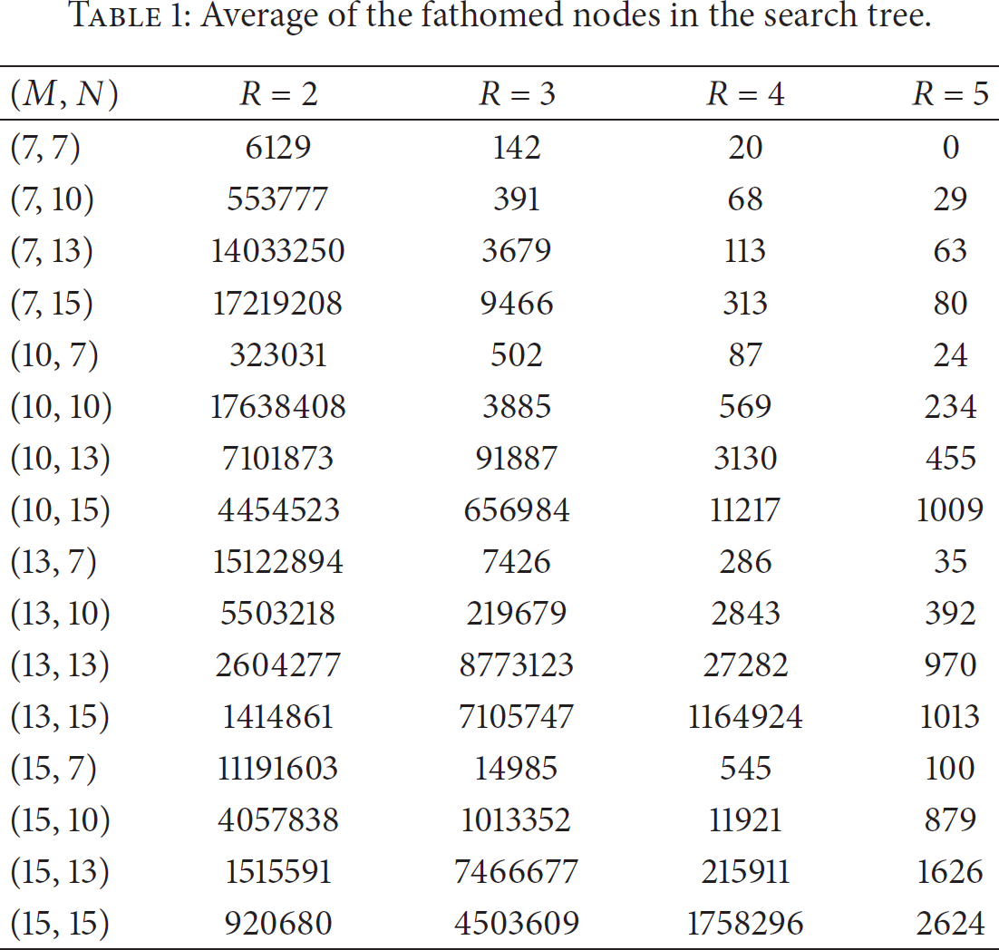
Table 2 gives an idea about the mean eliminated nodes by the two proposed properties. In Table 2, the first column represents the size of the grid. The second, fourth, sixth, and eighth columns contain the mean of nodes eliminated by the first property for $R = 2$ , $R = 3$ , $R = 4$ , and $R = 5$ , respectively. The third, fifth, seventh, and ninth columns contain the mean of nodes eliminated by the second property. From this table, we observe that the two properties have an important role in reducing the fathomed nodes. However, their importance varies according to the sensing range and the problem size. In fact, the mean of eliminated nodes increases when the grid size is large while the sensing range R is small. Nevertheless, it decreases when the sensing range is large.

Table 2

Mean of the eliminated nodes.

$(M$ , N)	$R = 2$		$R = 3$		$R = 4$		$R = 5$
$(M$ , N)	$P r_{1}$	$P r_{2}$	$P r_{1}$	$P r_{2}$	$P r_{1}$	$P r_{2}$	$P r_{1}$	$P r_{2}$
(7, 7)	3975	2087	23	36	3	0	0	0
(7, 10)	641858	222329	146	102	8	5	2	0
(7, 13)	22736250	6299444	1960	1406	20	28	5	1
(7, 15)	24516300	7942545	6474	3263	71	126	7	5
(10, 7)	351072	126614	175	161	9	9	1	0
(10, 10)	21931507	6464089	2474	1361	144	162	28	14
(10, 13)	9608302	2946136	81159	34868	1234	981	45	103
(10, 15)	8025261	2536092	882544	317526	7586	4622	299	324
(13, 7)	24619290	8009267	5475	3441	89	99	19	0
(13, 10)	11547112	2856468	234931	105072	1429	1166	138	148
(13, 13)	6479998	1530140	12832925	4660130	19822	11564	354	340
(13, 15)	4308342	916808	11073074	3650293	1715195	588276	470	307
(15, 7)	17365939	5561607	12961	7687	183	234	15	15
(15, 10)	8132338	2128375	1284577	503507	7628	5426	162	373
(15, 13)	3942029	907265	12143771	4026823	197663	96653	782	617
(15, 15)	3300098	692202	6851489	2114096	1888873	840005	1220	925

Table 3 represents the percentage of problems which are solved optimally by the B&B algorithm. We observe from Table 3 that the percentages of optimally solved problems depend on the sensing range. In fact, when the problem size increases and the sensing range decreases, then the percentage of the optimally solved problems decreases. However, when the problem size increases and the sensing range increases, then the percentage of the optimally solved problems increases.

Table 3

Percentage of optimally solved problems by the B&B algorithm.

R	(7, 7)	(7, 10)	(7, 13)	(7, 15)	(10, 7)	(10, 10)	(10, 13)	(10, 15)	(13, 7)	(13, 10)	(13, 13)	(13, 15)	(15, 7)	(15, 10)	(15, 13)	(15, 15)
2	100	100	57	0	100	0	0	0	28	0	0	0	0	0	0	0
3	100	100	100	100	100	100	100	100	100	100	0	0	100	100	0	0
4	100	100	100	100	100	100	100	100	100	100	100	100	100	100	100	100
5	100	100	100	100	100	100	100	100	100	100	100	100	100	100	100	100

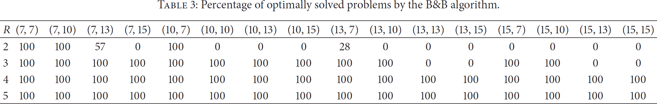
Figure 6 presents the mean computation time spent solving a problem with the B&B algorithm. The mean computation time of the grid size, for each R value, is determined by summing the computation times of the 7 generated instances corresponding to the 7 tested placements of the sink, and then by dividing the obtained value by 7. From this figure, we observe some mean computation times equal to 3600 seconds. This result allows us to conclude that the delivered solutions of these instances may not be optimal unlike the remaining instances which have a mean computation time less than 3600 seconds.

Figure 6

The mean computation time (in seconds) to solve a problem by the B&B algorithm.

Figure 7 represents the mean computation time to solve a problem with the integer linear model proposed by Rebai et al. [22]. If we compare the results of Figure 6 to those of Figure 7, three main observations can be derived.

Figure 7

The mean computation time (in seconds) to solve a problem by the linear model of Rebai et al. [22].

The first of those is about the total number of the instances having a mean computation time equal to 3600 seconds. In fact, in Figure 6, we observe fewer instances with a mean computation time equal to 3600 seconds.

The second concerns the mean computation time of the optimally solved instances. From the two figures, we observe that most of the instances, which are solved optimally by the B&B algorithm, have a mean computation time less than the mean computation time obtained by the integer linear model.

The third is about the impact of the sensing range on the mean computation time. In fact, for the two developed methods (i.e., the B&B algorithm and the integer linear model in Rebai et al. [22]), we observe that when the sensing range increases the mean computation time decreases. In the case of $R = 5$ , the two methods present roughly similar results.

From the results of Figures 6 and 7, we can conclude that the B&B algorithm results dominate the linear model results. We note that 74% of the tested instances are solved optimally by the B&B algorithm while only 69% of the tested instances are solved optimally by the linear model. This result allows us to confirm that the developed B&B algorithm is better than the integer linear model proposed by Rebai et al. [22].

7. Conclusion

In this paper, we have developed a B&B algorithm for the critical grid coverage problem in wireless sensor networks with connectivity constraint. Our contribution adds the constraint of connectivity between the deployed sensors to the general form of the critical grid coverage problem. The proposed method is able to provide appropriate solutions for the small and medium size problems. The simulation results show that the B&B algorithm is more efficient than the linear model proposed by Rebai et al. [22] for the same problem.

As perspectives, we aim to introduce infrastructure constraints (like walls) in the sensing field that may break the communication between the deployed sensors.

Footnotes

Conflict of Interests

The authors declare that there is no conflict of interests regarding the publication of this paper.

Acknowledgments

This work is supported by the SURECAP CPER Project (fonction de surveillance dans les réseaux de capteurs sans fil) and the Plateform CAPSEC (capteurs pour la sécurité) funded by Région Champagne-Ardenne and FEDER (fonds européen de développement régional).

References

Wang

Y. C.

C. C.

Tseng

Y. C.

Efficient placement and dispatch of sensors in a wireless sensor network

IEEE Transactions on Mobile Computing 2008 7 2 262 274

10.1109/TMC.2007.70708

Tseng

Y. C.

Wang

Y. C.

Cheng

K. Y.

An integrated mobile surveillance and wireless sensor (imouse) system and its detection delay analysis

Proceedings of the 8th ACM International Symposium on Modeling, Analysis and Simulation of Wireless and Mobile Systems (MSWiM '05)

October 2005

Montréal, Canada

178 181

Tseng

Y.-C.

Pan

M.-S.

Tsai

Y.-Y.

Wireless sensor networks for emergency navigation

Computer 2006 39 7 55 62

2-s2.0-33746369139

10.1109/MC.2006.248

Bai

Kumar

Xuan

Yun

Lai

T. H.

Deploying wireless sensors to achieve both coverage and connectivity

Proceedings of the 7th ACM International Symposium on Mobile Ad Hoc Networking and Computing (MobiHoc '06)

May 2006

Florence, Italy

131 142

2-s2.0-33748086475

10.1145/1132905.1132921

Burrell

Brooke

Beckwith

Vineyard computing: sensor networks in agricultural production

IEEE Pervasive Computing 2004 3 1 38 45

2-s2.0-2342482992

10.1109/MPRV.2004.1269130

Yun

Bai

Xuan

Lai

T. H.

Jia

Optimal deployment patterns for full coverage and k-connectivity (

k \leq 6

) wireless sensor networks

IEEE/ACM Transactions on Networking 2010 18 3 934 947

2-s2.0-77953684414

10.1109/TNET.2010.2040191

Ammari

H. M.

Das

S. K.

Centralized and clustered k-coverage protocols for wireless sensor networks

IEEE Transactions on Computers 2012 61 1 118 133

10.1109/TC.2011.82

Alfieri

Bianco

Brandimarte

Chiasserini

C. F.

Maximizing system lifetime in wireless sensor networks

European Journal of Operational Research 2007 181 1 390 402

2-s2.0-33847246366

10.1016/j.ejor.2006.05.037

Cerulli

Donato

R. D.

Raiconi

Exact and heuristic methods to maximize network lifetime in wireless sensor networks with adjustable sensing ranges

European Journal of Operational Research 2012 220 1 58 66

2-s2.0-84857910052

10.1016/j.ejor.2012.01.046

10.

Türkoǧullari

Y. B.

Aras

Altinel

I. K.

Ersoy

A column generation based heuristic for sensor placement, activity scheduling and data routing in wireless sensor networks

European Journal of Operational Research 2010 207 2 1014 1026

2-s2.0-77955560890

10.1016/j.ejor.2010.05.020

11.

Aneja

Y. P.

Chandrasekaran

Nair

K. P. K.

A branch-and-cut algorithm for the strong minimum energy topology in wireless sensor networks

European Journal of Operational Research 2010 204 3 604 612

2-s2.0-75149140374

10.1016/j.ejor.2009.10.032

12.

W.-C.

Liu

B.-H.

Tsai

M.-J.

The critical-square-grid coverage problem in wireless sensor networks is NP-complete

Computer Networks 2011 55 9 2209 2220

2-s2.0-79957460140

10.1016/j.comnet.2011.03.004

13.

Chakrabarty

Iyengar

S. S.

Cho

Grid coverage for surveillance and target location in distributed sensor networks

IEEE Transactions on Computers 2002 51 12 1448 1453

10.1109/TC.2002.1146711

14.

Andersen

Tirthapura

Wireless sensor deployment for 3D coverage with constraints

Proceedings of the 6th International Conference on Networked Sensing Systems (INSS '09)

June 2009

Pittsburgh, Pa, USA

Carnegie Mellon University

1 4

10.1109/INSS.2009.5409946

15.

Alam

S. M. N.

Haas

Z. J.

Coverage and connectivity in three dimensional networks

Proceedings of the 12th Annual ACM International Conference on Mobile Computing and Networking (MobiCom '06)

2006

Los Angeles, Calif, USA

346 357

16.

Shakkottai

Srikant

Shroff

N. B.

Unreliable sensor grids: coverage, connectivity and diameter

Ad Hoc Networks 2005 3 6 702 716

2-s2.0-24144491625

10.1016/j.adhoc.2004.02.001

17.

Liu

Xiao

Sun

Random coverage with guaranteed connectivity: joint scheduling for wireless sensor networks

IEEE Transactions on Parallel and Distributed Systems 2006 17 6 562 575

2-s2.0-33646231501

10.1109/TPDS.2006.77

18.

Tian

Georganas

N. D.

Connectivity maintenance and coverage preservation in wireless sensor networks

Ad Hoc Networks 2005 3 6 744 761

2-s2.0-24144479511

10.1016/j.adhoc.2004.03.001

19.

Zhao

Gurusamy

Lifetime maximization for connected target coverage in wireless sensor networks

IEEE/ACM Transactions on Networking 2008 16 6 1378 1391

2-s2.0-57949083359

10.1109/TNET.2007.911432

20.

Gupta

Zhou

Das

S. R.

Q. Y.

Connected sensor cover: self-organization of sensor networks for efficient query execution

IEEE/ACM Transactions on Networking 2006 14 1 55 67

2-s2.0-33144487909

10.1109/TNET.2005.863478

21.

Zhou

Das

Gupta

Connected k-coverage problem in sensor networks

Proceedings of the 13th International Conference on Computer Communications and Networks (ICCCN '04)

2004

Chicago, Ill, USA

373 378

22.

Rebai

Snoussi

Khoukhi

Hnaien

Linear models for the total coverage problem in wireless sensor networks

Proceedings of the 5th IEEE International Conference on Modeling, Simulation and Applied Optimization (ICMSAO '13)

April 2013

Hammamet, Tunisia

1 4

10.1109/ICMSAO.2013.6552637

23.

Chen

Koutsoukos

Survey on coverage problems in wireless ad hoc sensor networks

Proceedings of the IEEE SoutheastCon

March 2007

Richmond, Va, USA

24.

Younis

Akkaya

Strategies and techniques for node placement in wireless sensor networks: a survey

Ad Hoc Networks 2008 6 4 621 655

2-s2.0-39149099807

10.1016/j.adhoc.2007.05.003

R	(7, 7)	(7, 10)	(7, 13)	(7, 15)	(10, 7)	(10, 10)	(10, 13)	(10, 15)	(13, 7)	(13, 10)	(13, 13)	(13, 15)	(15, 7)	(15, 10)	(15, 13)	(15, 15)
2	100	100	57	0	100	0	0	0	28	0	0	0	0	0	0	0
3	100	100	100	100	100	100	100	100	100	100	0	0	100	100	0	0
4	100	100	100	100	100	100	100	100	100	100	100	100	100	100	100	100
5	100	100	100	100	100	100	100	100	100	100	100	100	100	100	100	100

R	(7, 7)	(7, 10)	(7, 13)	(7, 15)	(10, 7)	(10, 10)	(10, 13)	(10, 15)	(13, 7)	(13, 10)	(13, 13)	(13, 15)	(15, 7)	(15, 10)	(15, 13)	(15, 15)
2	100	100	57	0	100	0	0	0	28	0	0	0	0	0	0	0
3	100	100	100	100	100	100	100	100	100	100	0	0	100	100	0	0
4	100	100	100	100	100	100	100	100	100	100	100	100	100	100	100	100
5	100	100	100	100	100	100	100	100	100	100	100	100	100	100	100	100

A Branch and Bound Algorithm for the Critical Grid Coverage Problem in Wireless Sensor Networks

Abstract

1. Introduction

2. Related Works

3. Problem Description

4. Lower Bound

4.1. Definitions

4.2. Proposition

Proof.

5. Branch and Bound Algorithm (B&B)

5.1. The Initialization

Algorithm 1: The upper bound.

5.2. The Branching Scheme

5.2.1. Definitions

5.2.2. Property 1

Proof.

5.2.3. Property 2

Proof.

5.3. The Bounding Procedure

6. Computational Experiments

7. Conclusion

Footnotes

Conflict of Interests

Acknowledgments

References

R	(7, 7)	(7, 10)	(7, 13)	(7, 15)	(10, 7)	(10, 10)	(10, 13)	(10, 15)	(13, 7)	(13, 10)	(13, 13)	(13, 15)	(15, 7)	(15, 10)	(15, 13)	(15, 15)
2	100	100	57	0	100	0	0	0	28	0	0	0	0	0	0	0
3	100	100	100	100	100	100	100	100	100	100	0	0	100	100	0	0
4	100	100	100	100	100	100	100	100	100	100	100	100	100	100	100	100
5	100	100	100	100	100	100	100	100	100	100	100	100	100	100	100	100