Sage Journals: Discover world-class research

Abstract

A wireless sensor network (WSN) is a collection of sensor nodes that dynamically self-organize themselves into a wireless network without the utilization of any preexisting infrastructure. One of the major problems in WSNs is the energy consumption, whereby the network lifetime is dependent on this factor. In this paper, we propose an optimal routing protocol for WSN inspired by the foraging behavior of ants. The ants try to find existing paths between the source and base station. Furthermore, we have combined this behavior of ants with fuzzy logic in order for the ants to make the best decision. In other words, the fuzzy logic is applied to make the use of these paths optimal. Our algorithm uses the principles of the fuzzy ant colony optimization routing (FACOR) to develop a suitable problem solution. The performance of our routing algorithm is evaluated by Network Simulator 2 (NS2). The simulation results show that our algorithm optimizes the energy consumption amount, decreases the number of routing request packets, and increases the network lifetime in comparison with the original AODV.

1. Introduction

In WSNs all sensor nodes try to collect data and send sensing data to the base station (BS). The wireless communication uses a fixed node in the center of environment that is used to gather data from other sensor nodes called BS. Sometimes, source and destination are not in the neighborhood and they have multihop distance with each other where this distance leads to more energy consumption. The node energy consumption is the amount of energy each node consumes for sending/receiving data to/from other nodes. The summation of energy consumption by network nodes shows the network energy consumption. Since these energy sources are irreplaceable and have a straight effect towards the network lifetime, new protocols establishment or improvement in current protocols seems necessary for better energy saving in the network.

Routing is one of the most important protocols that consume energy in the network. Routing has been defined as a dynamic optimization task aiming at providing paths that are optimal in terms of some criteria such as minimum distance, maximum bandwidth, and shortest delay and satisfying some constraints such as limited power of nodes and limited capacity of wireless links. Routing is one of the major problems in the WSN and is one of the most interesting research fields in the communication network. The routing of the information is thus done locally and hop-by-hop. Each node independent of other decisions in other nodes and its past decision makes a new routing decision [1]. Routing usually directs based on the routing records that exist in each node routing table (RT) to various destinations in the network. The RT is a data table that is stored in node memory lists routs to special nodes. Nowadays, algorithms act differently to find the route between sender and destination; more algorithms only find a route and some routing algorithms find a multipath. The multiroute algorithms waste more network resources due to more message transmission as opposed to the single-path algorithms [2, 3].

Proactive, reactive, and hybrid [2, 4] are three main categories of routing algorithms. Proactive or, alternatively, the table-driven algorithms always show a fresh list of routes. Proactive algorithms have a slow reaction in the network with more failure and restructuring [2]. Examples of proactive algorithms are FSR [5] and DSDV [6]. The reactive or on-demand routing algorithm uses the flooding technique for finding only one path between the sender and destination. If the route exists before, the new route request will not accept them. High latency time in route finding is one of these algorithms' disadvantage and another is imposed overhead on the network due to the flooding technique; nevertheless it has less overhead compared to that for the proactive group. The most famous routing protocols of this group are DFS [7] and AODV [2, 4]. The third group is known as the hybrids. They are a combination of the reactive routing protocols and proactive routing protocols [4].

Ant colony [8, 9] is a standard solution for finding optimal path (from source to destination) that is proposed by Dorigo et al. in 1992 for solving optimization problems such as travelling salesman problem (TSP) with multiagents. By paying attention to inherent properties of routing, it will be suitable to be solved by the ant colony algorithm. Intelligent agent by the sensors will be able to sense events of the surrounding environment. ACO is based on the intellectual foundation that can easily be described in one sentence: ants select the best path among the existing barriers and constraints in nature to achieve food. This selection of a path is considered optimal among the different paths. Zadeh [10, 11] originally proposes the fuzzy set theory and it has been developed for expanded linguistic values. The linguistic values are terms, which are used instead of the numbers and fuzzy set theory [12]. The use of the fuzzy logic to optimize the metric used in routing approaches for WSNs is a promising technique since it allows us to combine and evaluate diverse parameters in an efficient manner. Moreover, several proposals have shown that the use of fuzzy logic in this kind of networks is a good choice due to the execution of the requirements that can be easily supported by sensor nodes, while it is able to improve the overall network performance [13]. Fuzzy logic consists of a decision system approach which works similarly to human control logic. It provides a simple method to reach a conclusion from imprecise, vague, or ambiguous input information [14].

In this paper, we aim to discover the optimal route in WSNs from the sources node to the BS. We are using intelligent ants that have some knowledge in the fuzzy logic and we call this FACOR algorithm. They will find the optimal path among all paths that may exist from the source to BS. In the first step, the source node sends ants to all neighbors; then each ant tries to find a route to BS. The ants will calculate the fuzzy amounts for their neighbors and the next hop based on these fuzzy amounts will be selected. This step will continue until the ants are able to find a route to BS. If an ant could not find this route in determined time, it kills itself. After that, the BS makes final decisions and determines the winner ant. The winner ant returns to its route and updates the routing table and some more information for all nodes on its route. We use the RREQ and RREP messages for modeling our ants. The simulation results show that this proposal reduces the number of packets needed to find the routes. By this manner we reduce the network bandwidth usage and decrease the amount of energy consumption because each node needs energy to send the packets. Also, our algorithm will be able to find optimal route and this route saves the network energy due to the shortest path selection. Furthermore, our algorithm also decreases the end-to-end delay time for sending and receiving packets. Giving attention to the above context, the network lifetime will increase.

Recently, many researches have been attempting to address this problem. Being attentive to the structural constraints that have WSN such as sensor limitation energy, developing efficient algorithms for routing seems necessary [4]. Sahani and Kumar in [15] proposed a novel routing approach using an ant colony optimization algorithm which uses artificial ants. Each ant chooses the next hop; moreover the pheromone concentration amount attends to the node's remaining energy. By this method, the ant will select a node with longer lifetime.

In [16] Suhonen et al. proposed an energy-efficient multihop routing protocol referred to as TUTWSNR (Tampere University of Technology WSN Routing) for wireless sensor networks. They use cost metrics to create gradients from the source to the destination node. The cost metrics consist of energy, node load, delay, and link reliability information that provide a trade-off between performance and energy usage. A node can query routes from its neighbors, which allows efficient recovery from route losses.

Okdem and Karaboga in [17] presented a novel routing approach using an ant colony optimization algorithm for wireless sensor networks consisting of stable nodes. The main goal of their study was to maintain network lifetime at its maximum. A multipath data transfer is also accomplished to provide reliable network operations, while considering the energy levels of the nodes. They also implement their approach on a hardware component to allow designers to easily handle routing operations in WSNs.

Kadri et al. in [18] are going to adapt the conventional ant routing algorithm for WSNs, by taking into consideration their traffic pattern and devices' constraints. The proposed protocol affects the task of route discovery to the BS which periodically launches forward ants over the network to discover routes and inform sensors about its location instead of letting each sensor do this task individually which consumes sensors' resources and decreases the network lifetime due to the broadcasting nature of the forward ants. They have also proposed execution of a handshake during the route discovery in order to secure links between each sensor and the BS, as the use of the underlying routing requests for the handshake has considerably saved the sensor's battery power with a good threshold of security [19, 20].

In [21] the authors designed an adaptive virtual area partition clustering routing protocol using ant colony optimization (AVAPCR-ACO), which used a virtual area partition scheme to cluster the network, and took advantage of the ant colony optimization to build a routing path among the cluster heads. In [22] the authors presented a mechanism for the wireless sensor network routing which can be more effective regarding the criteria of route length, end-to-end delay, and network node energy for the quality of mechanism service. The proposed method uses the ant colony-based routing algorithm and the local enquiry to find optimal routes. Also, a fuzzy inference system was used to determine the route quality which showed better performance compared with the equation of route quality. Chakraborty et al. [23] presented a novel trust-based congestion aware routing algorithm for WSNs in which the optimum route for data packet transfer is dynamically selected by the TC-ACO algorithm, on the basis of the trust, congestion level, and internodal distance of the sensor nodes.

The rest of the paper is organized as follows. In the next section, we describe the system model and problem specification. In Section 3, we illustrate our proposed algorithm and complete the representation of our solution with samples. Section 4 presents the simulation and results of simulation by different charts. In the final section, which is Section 5, we offer the conclusion and some recommendations for future works.

2. System Model and Problem Specification

In this section, we aim to describe our system model that has been used in this research and problems that we are going to address.

2.1. Network Model and Assumptions

In this research, we consider a sensor network consisting of N sensor nodes which are randomly deployed over an environment. Sensor nodes collect the sensing data from the surrounding environment and send these collected data to BS. We suppose our network model has been restricted by some assumptions.

Assumption 1.

All nodes are homogeneous and have unique identification and they are also initially deployed.

Assumption 2.

All nodes have the same initial energy.

Assumption 3.

In the initialization status, nodes do not have the information about each other such as location.

Assumption 4.

Each node acts as a router and also it is able to sense the surrounding environment.

Assumption 5.

Each node is able to communicate with other nodes in its transmission range. The maximum distance between two nodes is covered by the transmission range. The transmission range is determined by the signal strength. Thus, higher transmission powers will increase the number of nodes shared with the medium (connectivity degree) [24], and consequently, the probability of finding the destination among the node neighbors will be heightened. Of course, higher transmission range will have more disadvantages like collision problems. When two or more nodes want to send a packet at the same time over the same transmission medium or channel, collision will occur.

Assumption 6.

All nodes have a two-ray-amp antenna model and will be able to communicate with other nodes in its transmission range.

Assumption 7.

We used two different message delivery semantics: broadcasting and unicasting. In the broadcasting scheme, the sender sends the packets in its transmission range and all nodes in this transmission range receive these packets and send the packets to one special node.

2.2. Sensor Nodes and Energy Consumption Model

Sensors are usually wireless electronic elements and functions for sensing interactions. Sensors are located in the environment for data-gathering purposes (such as temperature, sound, vibration, pressure, motion, or pollutants) from the monitored area [25]. In recent years, with progress in technology, the wireless devices have been smaller, cheaper, and more powerful. Wireless sensor networks (WSNs) consist of sensor nodes that are designed with special purposes and applications (scientific, monitoring, or military purposes) [25].

In WSN, nodes are usually homogenous and consist of some units such as battery, sensors, transceiver, processor, and memory [26, 27]. The nodes send the collected data to the base station (BS). The BS is responsible for collecting data sent by the other nodes usually located in the center of the environment and sometimes has different units in comparison with the other nodes. Due to its interaction with other nodes and in some cases local data processing, the BS has power source with greater energy, larger memory, or maybe stronger processor. In the real system, all units of each node cooperate in doing delegated tasks that has effect on node energy consumption and in general on the network energy [26]. It should be noted that each node has a limited and irreparable energy source and if a node is turned off due to the completion of power source, it will reduce the connectivity degree and in some cases fragmentation in the network.

2.2.1. Sensor Nodes Behavior

In general, each node is placed in one of the two mechanisms based on the current state: active or sleep. In the active mechanism, a node uses efficient protocol on the network energy instead of turning off the transceiver for saving energy, while a node in the sleep mechanism has no interaction with other network nodes due to the fact that its transceiver is turned off and that the node energy consumption is lower [28].

In the active mechanism, each node will be in one of the three operational modes: transmit, receive, or idle. In the first mode (transmit), more node energies are consumed for turning on the transceiver and packet's transmit. In the second mode (receive), the node with its transceiver turned on receives a packet, demodulation, and decoding [29] where these operations (packet processing and turned-on transceiver) cause energy consumption in the node. After the packet's receiving or sending operations, a node is placed in the idle mode. In the idle mode, each node listens to the communication channel without any sending or receiving in an active manner. In this mode, some functions in the hardware can be switched off, but all circuits are maintained to be ready to operate. Figure 1 illustrates these states and communications.

Figure 1

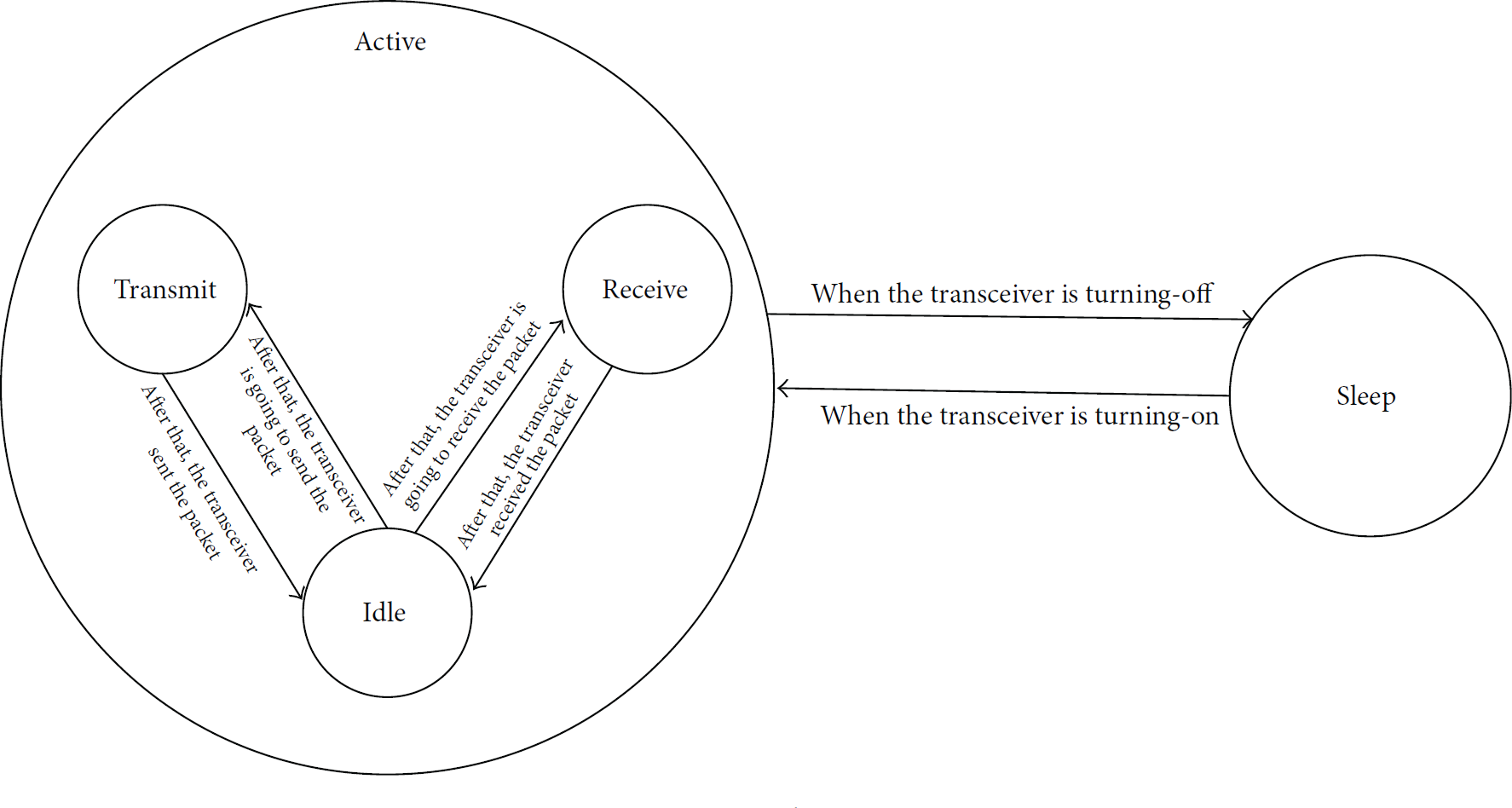
Node states.

2.2.2. Energy Consumption Model

The energy is one of the most important aspects in the WSNs; when a node loses its energy by any reason, in the worst condition, a big part of network may be misused due to fragmentation. The battery source provides all the energy that a node needs for doing its tasks. Currently, many different types of battery exist for the sensor nodes [30] that they come in various sizes, weights, amounts of energy saved, construction technology, and so forth. Table 1 shows some different types of batteries and technical specifications among them. Due to these limitations in the node battery source, generating an energy model for preventing more energy consumption in WSNs is necessary. The energy model only maintains the total energy and does not maintain the radio states [31]. We used the energy consumption model that has been shown in [32]. The energy spent for the transmission of a l-bit packet over distance d is calculated by the following equation:

\begin{array}{l} E_{Tx} (l, d) = E_{Tx-elec} (l) + E_{Tx-amp} (l, d) \\ = l \times E_{elec} + ({l \times ε}_{two-ray-amp} \times d^{4}) . \end{array}

(1)

The energy consumed by the transceiver for receiving a packet is calculated by the following equation:

\begin{matrix} E_{Rx} (l) + E_{Rx-elec} (l) = {l \times E}_{elec} . \end{matrix}

(2)

Table 1

Some of battery types and some technical specifications.

Battery type	Average voltage during discharge	Milli-amp hours (mAh)	Watt-hours (Wh)	Joules (J)	Weight
Alkaline long life	1.225	1150	1.41	5071	12
Alkaline long life	1.225	2122	2.60	9360	24

Nickel cadmium	1.2	300	0.36	1296	11
Nickel cadmium	1.2	1000	1.20	4320	11

Carbon zinc	1.1	320	0.35	1268	9.7
Carbon zinc	1.1	591	0.65	2340	19

The item $E_{elec}$ represents the energy consumption of transceiver dissipation and the ${l ε}_{two-ray-amp}$ represents the energy consumption for the amplifying transceiver, where $ε_{two-ray-amp}$ is a constant value and $d^{4}$ is a power loss for the channel model, depending on the distance between the transmitter and receiver. The transmit power ( $E_{Tx}$ ) is the power consumed by the transceiver to transmit a data packet. The size of the data packet determines the transmit power. The bigger the packet size, the more the power consumed. Receiving power ( $E_{Rx}$ ) is the energy used for receiving packet by the node. The energy cost $E (ρ)$ for a general route ρ is computed by the following equation:

\begin{matrix} E (ρ) = \sum_{i \in ρ} (E_{Tx}^{i} + E_{Rx}^{i}) . \end{matrix}

(3)

In this equation the final energy consumption amount is equal to the summation of $E_{Tx}^{i}$ and $E_{Rx}^{i}$ for each node with the identification i on route ρ. The route includes the sender and routers' node (intermediate nodes until the BS) without the BS.

2.3. WSN Protocols and Improvements

In this section, some protocols that are used in WSNs will be explained like AODV for routing, IEEE 802.11 for MAC layer, and CBR for traffic control. In the last subsection, we discuss all improvements where we are going to reduce the energy consumption amount by applying them in WSNs.

2.3.1. AODV Routing Overview

Ad hoc on-demand distance vector (AODV) is one of the most used reactive routing protocols for WSN. In the reactive routing, paths are determined only when needed [33]. The primary objectives of this protocol are (a) to broadcast discovery packets when needed, (b) to distinguish between local connectivity management (neighborhood detection) and general topology maintenance [34], and (c) to propagate information on node connectivity degree for its neighbors or other interest nodes. Figure 2 depicts the messages that are used in the AODV protocol. A node which is aware of its surrounding environment (e.g., neighbor nodes) locally broadcasts a HELLO message; also the route request (RREQ) packets are sent if a sender is finding a route to BS. In this case, the path is made by route reply (RREP) packet unicasting to sender.

Figure 2

AODV protocol messages.

The AODV uses the route discovery mechanism with broadcasting instead of the source routing. Each node has a local routing table (RT) for quick response time to requests and establishment. Each row of RT shows the next hop from this node to the destination. The route discovery process is implemented when a node needs to communicate with other nodes and route information does not exist in its RT. The protocol uses the sequence number for more maintenance of the routing information among nodes. This sequence number will cause the efficient use of network bandwidth by minimizing the network load for the control and data traffic.

When a node wishes to send data to the BS, the source node creates a RREQ packet. This packet contains the source node's IP address, source node's current sequence number, the destination IP address, and destination sequence number that are broadcast in the source transmission range. Broadcasting is done via flooding. Finally, this packet will receive a node that possesses a current route to the destination. Firstly, the receiver checks the RREQ packet. If the intermediate node has an entry in RT for the desired destination, the intermediate node will make a decision by comparing its entry sequence number with RREQ packet sequence number. If the intermediate node has not received this RREQ before, meaning that it is not the destination and does not have a current route to the destination and RREQ sequence number is bigger than saved sequence number, it rebroadcasts the RREQ [33, 34]. When the intermediate node is capable of replying, it means that it has a sequence number greater than or equal to that contained in the RREQ. If a node receives a packet with the same broadcast ID and source address, it drops this RREQ packet (sometimes maybe a node receives multiple copies of the same RREQ packet) [34].

Once an intermediate node receives a RREQ and its destination, the node sets up a reverse route entry for the source node in its RT. Reverse route entry consists of source IP address, source sequence number, number of hops to source node, and IP address of node from which RREQ is received. Using the reverse route, a node can send a RREP packet to the source. The RREP is unicast in a hop-by-hop model to the source [33]. While the PREP backward to the source, each intermediate node creates a route to the destination and sets up a forward pointer to the node from which the RREP comes.

Node 2, as Figure 3 shows, decided to send the packets to node 9. In the first step after node 2 checked its RT and it does not find any path to BS, it makes RREQ packets and broadcasts these packets. Nodes 1, 3, and 5 receive this packet and since these are not destinations, they will broadcast the RREQ packet for their neighbors. This event will be repeated for nodes 4, 6, 7, and 8. Finally, when node 9 receives this packet for the first time, it makes RREP and unicasts RREP hop-by-hop to node 2 and the intermediate nodes update its RT and create a route to the destination. After the routing discovery is finished, node 2 sends its data to node 9 on this discovered path.

Figure 3

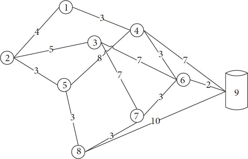
A sample of WNS.

2.3.2. MAC Layer

To avoid collision, the medium access control (MAC) protocols have developed and control how each node could access the channel. IEEE 802.11 is a distributed MAC scheme that works based on the carrier sense multiple accesses with collision avoidance (CSMA/CA). In this scheme, each node accesses the medium on a contention basis. Before a data transmission begins, the sender and receiver must have a RTS-CTS signaling handshake to reserve the channel [35]. A sender for sending a packet, firstly, with its transceiver senses the channel and looks up its network allocation vector (NAV). Therefore if the channel is free, it sends a RTS (request-to-send) to the destination node, and the destination with a CTS (clear-to-send) approves RTS receiving; otherwise it has to wait until the channel is busy. As the CTS is received by receiver, it can start the data transmission and destination, confirming that data are successfully received via acknowledgment (ACK) [35].

2.3.3. Traffic Protocol

The constant bit rate (CBR) service category is used to transport traffic connections at a constant bit rate, where there is an inherent reliance on the time synchronization between the traffic source and destination. The consistent availability of a fixed quantity of bandwidth is considered appropriate for the CBR service. Cells which are delayed beyond the value specified by the cell transfer delay (CTD) are assumed to be significantly of less value to the application. In the CBR, bandwidth guarantees the peak cell rate of the application.

2.3.4. Improvement in the Original AODV Routing

As it has been mentioned, the AODV is one more used network routing protocol. The AODV protocol uses the message broadcasting delivery with the flooding technique. Finding the methods for reducing energy consumption will cause an increase of the network lifetime and it will be an improvement for WSNs. The following objectives are set in this research.

Improvement 1. In the original AODV, each sender broadcasts RREQ packets. This is costly for the network and it causes more energy consumption and, furthermore, busy network bandwidth. Reducing the number of RREQ packets will be an improvement, which decreases the energy consumption amount, increases network lifetime, and controls the overhead in the network.

Improvement 2. By focusing on the broadcasting of the RREQ packet by each node, for all its neighbors in the original AODV, several routes may exist between the sender and BS. Due to this reason, several RREP packets tend to return to the sender. We try to reduce the number of RREP packets and it proves to be another improvement.

Improvement 3. Another improvement is selecting the best node among the neighbor senders. If an algorithm involves some extra parameters, in addition to the neighborhood like remaining energy, connectivity degree, distance, etc., for selecting next hop, these extra parameters, due to the increased packet delivery speed, will increase energy saving in the network. Also, this technique avoids the route discovery repetition.

3. Proposed Solution

In this section, our proposed algorithm will be explained. In Section 3.1, we describe utilization techniques (fuzzy logic and ant colony) in this research. Section 3.2 clears the proposed algorithm by the pseudocode and the last section illustrates a sample of our algorithm.

3.1. Ant Model and Fuzzy Logic Model

When a node wishes to send collected data to BS as has been stated in Section 2.3.1, it makes a RREQ packet and broadcasts it to all neighbors. We used two kinds of ants: forward and backward ants that have been presented by FAnt and BAnt. RREQ packet is used for modeling the FAnt and BAnt. In this research, we have several FAnts (depending on the source neighbor's number) and a BAntthat will be discussed in the next sections. FAnt tries to find a route from the sender to the BS (a FAnt is launched from the source and intermediate nodes until the BS). While FAnt moves forward, it saves the list of nodes that has been visited in its memory and tries to avoid traveling the same node and BAnt fixes this route. In our algorithm, we restricted and targeted the number of RREQ packets (FAnts) sent by each node in compared with the original AODV. The winner FAnt makes a BAnt with the same parameters and BAnt returns to the source and updates RT and pheromone concentration amount for each node in its path. We used the pheromone rules the same way as in [36].

BAnt when traversing from a node will increase the pheromone as shown in (4), where α is the variable parameter, $hm$ represents the maximum hops between sources to destination, $hc$ is the remaining hops to destination, and $En$ represents node remaining energy. We added the node remaining energy to this equation based on the reason that the ants select the node with greater power. Consider

\begin{matrix} Δ τ = α \times (hm - hc) \times En . \end{matrix}

(4)

When the node with identifier n transmits the packet, it updates the pheromone concentration amount with the following equation:

\begin{matrix} τ_{n} = (1 - ρ) \times τ_{n} + Δ τ, \end{matrix}

(5)

where ρ is the pheromone evaporation (pheromone amounts evaporate very soon when no ants traverse from this path) coefficient, the range of ρ is

[0,1]

, and

1 - ρ

is the pheromone residue factor. We added a structure to FAnt and BAnt to save the traveling path in addition to the original fields which used AODV for RREQ and RREP packets.

Fuzzy system consists of three parts [37]: fuzzification, inference engine, and defuzzification. Figure 4 shows the fuzzy system factors used in this paper. In a fuzzy logic-based system, calculations are performed by an inference engine. In order to select the inference engine, we have studied two widespread approaches presented in the literature: Mamdani [38] and TSK [39]. Here we use the Mamdani inference engine. The input of a Mamdani fuzzy logic system is usually a crisp value.

Figure 4

Fuzzy logic system model.

(i) Fuzzification. Input variables by membership functions should be converted to linguistic values to determine the membership degree. The outputs of this stage are fuzzy values that can be processed by the inference engine.

(ii) Inference Engine. At this stage, the input fuzzy values from the previous stage apply to all fuzzy rules that are kept in the fuzzy database by the inference engine. All rules that are adaptable to input parameters will be activated and then the output of all activated rules will be aggregated. All rules are in the IF-THEN form and here we have 64 different rules, where Table 2 shows some samples of the rules used in this research.

Table 2

Some of uses rules.

Rules database
Rule number	ReE	Dis	ConD	PheA	Out
1	High	Near	High	High	Very good
2	High	Moderate	Medium	High	Good
3	Low	Far	Low	Low	Very bad
4	High	Far	High	Low	Bad

(iii) Defuzzification. The inputs of this phase are those linguistic values and the outputs are nonfuzzy values. Mamdani uses the centroid technique which tries to determine the point where a vertical line divides the combined set into two equal parts. We use the defuzzification formula as follows:

\begin{array}{l} Y = \sum_{i = 0}^{63} ((5 * {Ph}_{i}) + (1.5 * {Re}_{i}) \\ + (1.5 * {CD}_{i}) + (1 * {Dis}_{i})) * O_{i}, \end{array}

(6)

\begin{array}{l} w = \frac{Y}{\sum_{j = 0}^{63} O_{j}} . \end{array}

(7)

In (6) ${Ph}_{i}$ is the pheromone concentration amount, ${Re}_{i}$ is the remaining energy, ${CD}_{i}$ is the connectivity degree, ${Dis}_{i}$ is the destination between 2 nodes, and $O_{i}$ is the output value for rule number i (we will have a full discussion about these parameters in the section below). Finally, a fuzzy logic value is obtained for all 64 rules by (7) (Y is divided by the whole position output of all rules).

3.1.1. Energy Optimized Parameters

If FAnts act intelligently in choosing the next node, we will be nearer to our aim. We aim to assist FAnts in choosing the next node with fuzzy logic. By this method, the FAnts, in addition to the pheromone concentration amount for choosing next node, will use the extra parameters, where these parameters contribute to the more intelligent choices. In this proposal, we focus our attention on factors such as remaining energy of each node as well as the connectivity degree of the same node (the number of neighbors), the distance of node to its neighbors, and then its pheromone concentration amount. These factors are briefly discussed as follows.

(i) Remaining Energy. We know that each node has a battery with limited power, and energy saving for batteries is essential for node survival and network maintenance. On the other hand, as we will select the node with the highest remaining energy, the network lifetime will increase. We assume impact factor 1.5 for the remaining energy.

(ii) Connectivity Degree. The numbers of node neighbors which are in the transmission range of the node are defined as the connectivity degree of the node. This is important because if a node with a higher degree is elected, firstly, with higher probability we can find the destination with this node and, secondly, perhaps the destination is one of its neighbors that can decrease the length of the path as well as reducing the energy consumption of the whole network. Also, we use impact factor 1.5 for connectivity degree.

(iii) Distance of Node. As the distance between two nodes within the transmission range grows, they need more energy to send/receive data, but with high probability the destination is nearest to this node. The distance between the current node to this neighbor calculates with (8) that in this formula $(x, y)$ shows the location of current node and $(x_{n}, y_{n})$ is the location of the destination (here one of current node neighbor). This list has a row for each current node neighbor. We use the impact factor 1 for it. Consider

\begin{matrix} N - distance = \sqrt{{(x_{n} - x)}^{2} + {(y_{n} - y)}^{2}} . \end{matrix}

(8)

(iv) Pheromone Concentration Amount. It is the most important factor for selecting the next neighbor node in the network environment. Surely, the ants will select the neighbor node with the higher pheromone concentration amount because more biotypes use this path for arriving to their destinations in the past. The impact factor for it is equal to 5.

3.1.2. Linguistic Values and Membership Functions

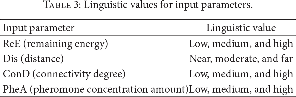
As Table 3 shows, each factor is being presented by three linguistic values. Linguistic values, namely, low, medium, and high, are used for input parameters of the remaining energy, connectivity degree, and pheromone concentration amount. The use of near, moderate, and far for distance; also the values of very bad, bad, good, and very good are used for output parameters that are indicated by Table 4.

Table 3

Linguistic values for input parameters.

Input parameter	Linguistic value
ReE (remaining energy)	Low, medium, and high
Dis (distance)	Near, moderate, and far
ConD (connectivity degree)	Low, medium, and high
PheA (pheromone concentration amount)	Low, medium, and high

Table 4

Linguistic values for output parameter.

Output parameter	Linguistic value
Out (output)	Very bad, bad, good, and very good

Figures 5, 6, 7, and 8, respectively, show the membership functions of the remaining energy, connectivity degree, distance, and pheromone concentration amount. Figure 9 depicts the membership function of the output unit before the defuzzification of results. The input parameters are taken by a membership function with degree one and it becomes a fuzzy value.

Figure 5

Battery level fuzzy sets.

Figure 6

Distance fuzzy set.

Figure 7

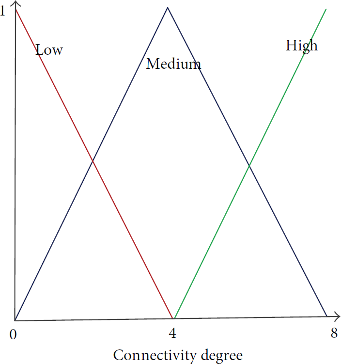
Connectivity degree fuzzy set.

Figure 8

Pheromone fuzzy set.

Figure 9

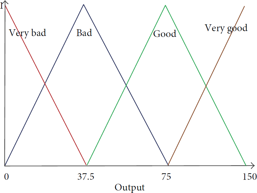
Output fuzzy set.

3.2. Proposed Algorithm

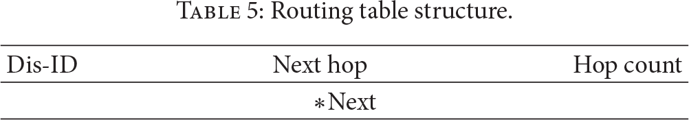
In our algorithm, each FAnt tries to find the optimal path from the source to destination. In the WSN destination, there is always a BS. The ant for delivering a packet has to move to some nodes that are in the source neighborhood. Each node keeps different structures such as routing table (RT) and neighbors' list (NL). RT (see Table 5) contains special information about node neighbors. The size of RT is different for each node, but for all nodes the fields are similar. In this structure, the first field indicates the destination node identifier (Dis-ID), the second indicates the next hop identifier, and the last, the hop count, shows the traveled hop from the source to this node. NL is a structure that keeps the node neighbors.

Table 5

Routing table structure.

Dis-ID	Next hop	Hop count

*Next

Due to the static structure of the WSN, the identified path by ants is always an optimal path. The optimal path is one of the existing paths between the source and destination with the fastest speed, the lowest cost (such as node energy consumption), and the most stable packet delivery. If we presume that nodes have had a little movement, the selected path needs to be reselected in the next communication. We presume in this paper that all nodes are fixed. When the path is discovered, the data are transmitted on this path between the source and destination. It is clear that the data transmission on a fixed path will cause more energy consumption for routers and sometimes may cause some routers to lose all the power. Our algorithm will repeat the path discovery operation in the determined time to prevent this. Below, we describe our algorithm in two phases and three steps.

Phase 1 (identification).

Step 1 (neighbor's identification). After that, a node which decides to send a packet to the determined receiver or BS triggers this step. The sender broadcasts a HELLO message in the transmission, rings the identifying neighbors, and creates or updates its NL. By this message the sender sends its identifier (S-Id) and sets M-Type (see Table 6). We used the M-Type field to distinguish between messages broadcasted by sender to neighbors and reply message sent by the receiver to sender. Each receiver which receives this message changes the M-Type field values by one and unicasts its identifier (N-Id) for the sender. When the primary sender receives the HELLO message with M-Type value equal to one, firstly, it searches in its NL and if this node is not identified before, this node is added in NL. Pseudocode 1 depicts the pseudocode that we used.

Table 6

Routing table structure.

S-Id/N-Id

M-Type

Pseudocode 1: Pseudocode for Step 1.

SendHELLO (node i, packet P) {

P.id = i;

P.M-Type = 0;

Broadcast p;

}

ReceivedHELLO (packet P) { //node j received packet P from node i

If (P.M-Type == 0) {

P.id = current-id;

P.M-Type = 1;

Unicast P; // packet P send for sender node;

}

Else If (P.M-Type == 1) {

Rez = Search P.id in current node neighbors-list (NL)

If (Rez == False) {// Node don't exist in current node Neighbor-list

Create new neighbor row;

NL.N-ID = P.id;

}

Step 2 (route discovery). In this step, as Pseudocode 2 illustrates, our algorithm executes based on the fact that the node is the source or intermediate node. If this node is the source, it sends the FAnts to all neighbors that exist in its NL by unicasting. If this node is an intermediate node, FAnt is unicast for the next hop that has been recognized by the fuzzy logic system (firstly, we went to Step 1 to identify its neighbors and update its NL and then for all neighbors in its NL we calculated the fuzzy amount and selected the node with the biggest fuzzy amount as the next hop). Each FAnt aggregates this new fuzzy amount that is obtained for the next hop with the sum of other fuzzy amounts obtained from other intermediate nodes, adds the current node identifier to the list of traveled nodes, and also has in its memory a field for saving the fuzzy amount.

Pseudocode 2: Pseudocode for Step 2.

SendFAnt (Forward-Ant-Packet FAnt, Node Next-Hop, Node Current-Node-ID) {

If (current-Id == source) {

NLPointer = First;

While (NLPointer != NULL) {

Create Forward-Ant-Packet FAP;

FAnt.id = NLPointer.N-ID;

FAnt.dis = Destination;

Unicast FAP;

NLPointer = NLPointer.next;

}

Else {

FAnt.dis = Next-hop;

Unicast FAnt;

}

ReceivedFAnt (Forward-Ant-Packet FAnt) {

If (FAnt.dis != current-Id) {

Create HELLOMESSAGE packet P;

SendHELLO (current-Id, P);

NLPointer = First;

J = 0;

FuzzyArray $[N e i g h b o r s - C o u n t]$ ;

FuzzyID $[N e i g h b o r s - C o u n t]$ ;

While (NLPointer != NULL) {

FuzzyArray $[j]$ = Get-Fuzzy-Amount (NLPointer.N-ID);

FuzzyID $[j]$ = NLPointer.N-ID;

NLPointer.N-ID = NLPointer.Next;

}

Max-amount = FuzzyArray $[0]$ ;

Max-id = FuzzyID $[0]$ ;

find = 0;

For (int k = 1; $k < l$ ; K++)

If ((Max-amount < FuzzyArray $[k]$ ) And (FuzzyID $[k]$ does not exist in FAnt.Path-list)) {

Max-amount = FuzzyArray $[k]$ ;

Max-id = FuzzyID $[k]$ ;

find = 1;

}

If ((find == 1) Or (FuzzyID $[k]$ does not exist in FAnt.Path-list)){

FAnt.Nexthopee = maxid;

Add current-Id to FAnt.Path-list;

FAnt.fuzzy-amount += Max-amount;

SendFAnt (FAnt, Max-id);

}

Else if ((find == 0) Or (FuzzyID $[0]$ does not exist in FAnt.Path-list)){

FAnt kill itself;

}

Else if (FAnt.dis == current-Id) {

Wait (R-Timer); // wait till all ant arrive

Select winner ant;

Delete other FAnts;

Create Backward-Ant Packet BAnt;

BAnt.Id = FAnt.Id;

Next-hop = FAnt.Path-list $[0]$ ;

Delete FAnt.Path-list $[0]$ ;

BAnt.Dis-list = FAnt.Path-list;

BAnt.Nexthop = Next-hop;

SendBAnt (BAnt, Next-hop);

}

Get-Fuzzy-Amount (Node id) {

En = get-node-energy (id);

Dist = get-distance (Current-Node, id) by (8);

Pher = get-Pheromone (id);

Conn = get-connectivity (id);

Calculate fuzzy amount based on (7);

Return fuzzy amount;

}

When the FAnt has reached its destination, if the current node identifier is equal to the BS identifier, we start a timer and wait until other FAnts arrive at the BS. After this timer is expired, the BS selects the best FAnt based on these fuzzy amounts that each ant has its memory, kills other FAnts, creates a BAnt, copies the FAnt path (path-list) in the BAnt path (Dis-list), and goes to the next step. The BS for selecting the winner FAnt, firstly, reads the hop count values from each FAnts memory and takes it in a list for each FAnt independently. Then, with this tip in mind, the FAnt with a shorter hop count is better than FAnts with the largest hop count and it deletes the FAnts with a larger hop count value. Later, the FAnts with equal hop count will remain (it is possible that a FAnt will be reminded that it has the shortest hop count); the final work for selecting the winner FAnt selects the FAnt with the largest fuzzy amount. The theory behind this selection is that this path is the optimal path with the shortest hops, fastest packet delivery, and lowest energy consumption. Also, in this step, if each FAnt finds a loop or cannot find a path to the destination, the FAnt will kill itself.

Step 3 (rollback). As Pseudocode 3 shows, BAnt returns to the source hop-by-hop and updates RT and pheromone concentration amount of all nodes in its path. The traveling path has been saved in the ant memory (Dis-list). Other ants which prevent higher network energy consumption will be killed by the BS in the next step. The latest identifier in this list is the identifier of the first node that the BAnt should visit. The BAnt sets its destination, removes this identifier, increases the pheromone amount (Ph-Amount field value) with (4), updates the RT entry for this route, and moves to its destination. This work will continue until this list becomes empty, and when this list becomes empty the BAnt will surely arrive at the source node.

Pseudocode 3: Pseudocode for Step 3.

SendBAnt (Backward-Ant Packet BAnt, Node Next) {

Unicast (BAnt, Next);

}

ReceiveBAnt (Backward-Ant Packet BAnt) {

If (BAnt.Nexthop == Source-Node-ID) {

Update source node RT;

Increase Ph-Amount for source by (4)

Delete BAnt;

Start Repeat-Timer

}

Else {

Update current node RT entry;

Increase Ph-Amount for current node by (4)

Next-hop = BAnt.Dis-list $[0]$ ;

Delete BAnt.Dis-list $[0]$ ;

BAnt.Nexthop = Next-hop;

SendBAnt (BAnt, Next-hop);

}

In this step, we used the acknowledgment system to guarantee message delivery. Each node that currently has BAnt saves a copy of it in its memory, then sends it, and waits until it receives an acknowledge packet from the receiver node in determined time; if the sender receives this acknowledge packet it will remove the BAnt's copy; otherwise it will resend this packet.

Phase 2 (relaxing).

Finally, nodes do not need to do something new to send the data packets to the destination (Pseudocode 4). They are looking at their RT and select the next hop. Notably, when the packet arrives at a node, it increases its pheromone amount (Ph-Amount field value) by (5). In this phase, if, by any reason, such as the node dies or due to the node movement, the path will be broken or if the repetition timer is expired, the source will repeat this algorithm and find another optimal path between the source and destination (BS). This operation increases the network lifetime as illustrated in Pseudocode 3.

Pseudocode 4: Pseudocode for Phase 2.

ReceiveData (Data-packet dp) {

Increase pheromone amount by (5)

find next hop on it RT

check next-hop status

if (next-hop be alive)

Unicast (dp, next-hop);

else if (next-hop not be alive or Repeat-Timer is expired)

repeat route discovery algorithm

}

3.3. FACOR Sample

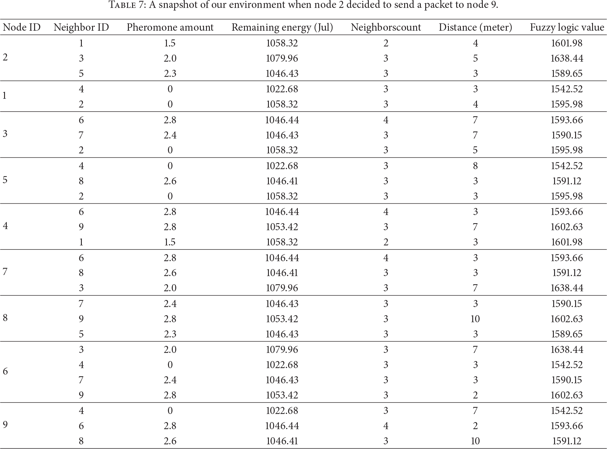
Figure 10 illustrates the example of the WSN. As this Figure shows, the distance between two neighbors is written on their edge. For example, node number 2 will send a packet to node number 9 (BS). Table 7 illustrates a snapshot of the environment when node 2 decides to send a packet to 9. As this table shows, each node (informing all four basic factors in Section 3.1.1) will decide for the next hop. The last column in this table shows the calculated fuzzy logic values for all nodes at a time of simulation. We should pay attention to this point that fuzzy logic values will be calculated independently for each ant when the ant wants to select the next hop in all simulation times.

Table 7

A snapshot of our environment when node 2 decided to send a packet to node 9.

Node ID	Neighbor ID	Pheromone amount	Remaining energy (Jul)	Neighborscount	Distance (meter)	Fuzzy logic value
2	1	1.5	1058.32	2	4	1601.98
	3	2.0	1079.96	3	5	1638.44
	5	2.3	1046.43	3	3	1589.65

1	4	0	1022.68	3	3	1542.52
1	2	0	1058.32	3	4	1595.98

3	6	2.8	1046.44	4	7	1593.66
	7	2.4	1046.43	3	7	1590.15
	2	0	1058.32	3	5	1595.98

5	4	0	1022.68	3	8	1542.52
	8	2.6	1046.41	3	3	1591.12
	2	0	1058.32	3	3	1595.98

4	6	2.8	1046.44	4	3	1593.66
	9	2.8	1053.42	3	7	1602.63
	1	1.5	1058.32	2	3	1601.98

7	6	2.8	1046.44	4	3	1593.66
	8	2.6	1046.41	3	3	1591.12
	3	2.0	1079.96	3	7	1638.44

8	7	2.4	1046.43	3	3	1590.15
	9	2.8	1053.42	3	10	1602.63
	5	2.3	1046.43	3	3	1589.65

6	3	2.0	1079.96	3	7	1638.44
	4	0	1022.68	3	3	1542.52
	7	2.4	1046.43	3	3	1590.15
	9	2.8	1053.42	3	2	1602.63

9	4	0	1022.68	3	7	1542.52
	6	2.8	1046.44	4	2	1593.66
	8	2.6	1046.41	3	10	1591.12

Figure 10

Sample of our algorithm mechanism.

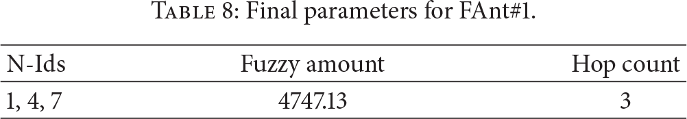
Tables 8, 9, and 10 determine the final parameters that each FAnt has when it reaches the receiver (node 9) at the end of Phase 2. If node 2 decides to send a packet, it must follow our steps. Based on these tables in the receiver, FAnt 3 wins this competition and returns to sender for updating RTs. As we see in these tables, the fuzzy amount for FAnt 2 is bigger than the other two, but due to less hops count, FAnt 3 wins.

Table 8

Final parameters for FAnt#1.

N-Ids	Fuzzy amount	Hop count
1, 4, 7	4747.13	3

Table 9

Final parameters for FAnt#2.

N-Ids	Fuzzy amount	Hop count
3, 7, 6, 9	6424.88	4

Table 10

Final parameters for FAnt#3.

N-Ids	Fuzzy amount	Hop count
5, 8, 9	4783.39	3

Figure 10 shows the result of our algorithm on a sample network. Figures 10(a) to 10(d) illustrates the paths that each ant takes for reaching the receiver. Each FAnt has its path and saves this path. The receiver sets a timer when it receives the first FAnt and waits for all FAnts. When the timer expires, the receiver selects the best FAnt, kills others, and makes BAnt (Figure 10(e)). The BAnt returns to the source and updates RT for each node in its path. Probably some FAnts are not able to find a path to the receiver (because the resulting graph of the network connectivity is not always a connected graph). In this situation the FAnt will kill itself when finding deadlock and then the receiver will not wait for many times because of its timer.

4. Simulation and Result

The performance of algorithm is evaluated by network simulator 2 (NS2) [40] and is implemented in two scenarios. NS2 is one of the most famous and most widely used network simulators. In this simulation, we consider a network with 10, 20, 30, 40, 50, 60, 70, and 80 nodes that are randomly placed in a dimension of 1500 M * 1500 M area. Each simulation is running for 180 seconds of the simulation time. As aforementioned, we implemented two scenarios based on the node transmission range (100 M transmission range for scenario 1 and 300 M transmission range for scenario 2) and repeated the simulation for different number of nodes in each scenario. Table 11 lists the simulation parameters. All nodes were taken randomly in the environment and we only controlled the hop count in the simulation time.

Table 11

Simulation parameters.

Simulation environment
Area	1500 m²
Simulation time	180 seconds
Nodes	10, 20, 30, 40, 50, 60, 70, and 80
Nodes placement	Random
Mobility model	Fix
Traffic	CBR
MAC layer	IEEE 802.11
Transmission range	100 m and 200 m
Maximum battery power (initial energy)	1150 J
$E_{Rx}$	1.42681e − 12, 8.91754e – 10 wat
$E_{Tx}$	0.281838 watt

Focusing on the different node states, we assume different parameters for each state as shown by Table 11. We have two different values for field, first $1.42681 e - 12$ when the transmission range is 100 M and then $8.91754 e - 10$ for 200 M transmission range.

4.1. Energy Consumption

The amount of energy consumption in the network depends on the amount of energy required to transmit a message from a sender to a receiver. Surely, if a proposed algorithm is able to reduce energy consumption in the network, the network lifetime will increase. The numerical values that we used for both scenarios are illustrated in Table 11. The results of energy consumption for both scenarios are shown in Figure 11. There are many effective parameters on energy consumption in the network such as network setup time, routing setup time, CPU processing, transmitting packets, and receiving packets, and in this proposal we measure the final energy consumption for the network at the end of simulation time.

Figure 11

Results of our algorithm in two different scenarios.

As this figure illustrates, when we have a larger transmission range, due to this larger transmission range, connectivity degree increases, energy consumption is lower, and the network lifetime will increase. We measured the algorithm of the energy consumption after 10 times for each group in different scenarios; also we assumed that the receiver is two hops away from the sender. Another result shows that, by increasing the node number for bigger transmission range, the energy saving will be better in the network (due to increased connectivity degree).

Here, our algorithm has been compared with the original AODV. As Figure 12 demonstrates, our algorithm has optimal performance compared to the original AODV and, approximately, they operate the same way when the number of nodes is lower than 20. This figure shows the AODV with message broadcasting, but our algorithm also shows a better performance in comparison with the AODV without the message broadcasting. As this figure shows, our algorithm for 50 nodes consumed about 500 J energy, but AODV in the same condition consumed about 700 J energy. In this comparison, also we assumed 100 M transmission range and two hops distance between the sender and receiver.

Figure 12

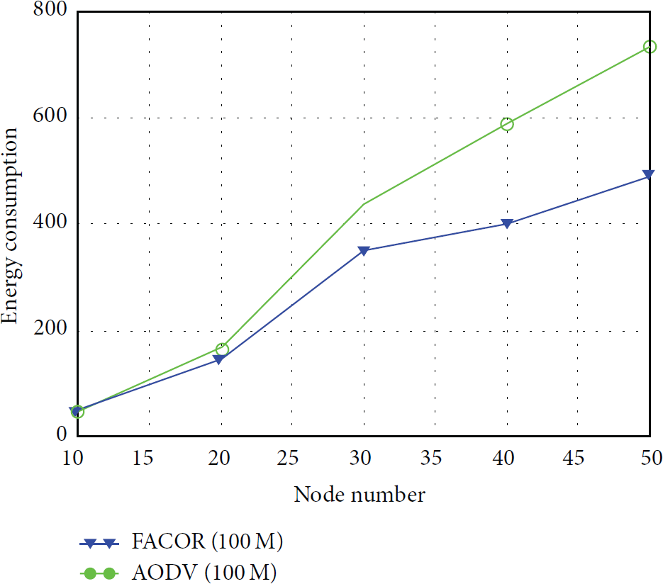
The energy consumption of route discovery.

4.2. Routing Setup Time

This represents the time spent by a protocol to discover routes from sender to receiver. It is the time since the first discovery packet is sent till the sender has a route to the receiver. By this field, we will measure the time from the moment that the discovery phase starts until the moment that the winner ant updates all nodes in its path to sender.

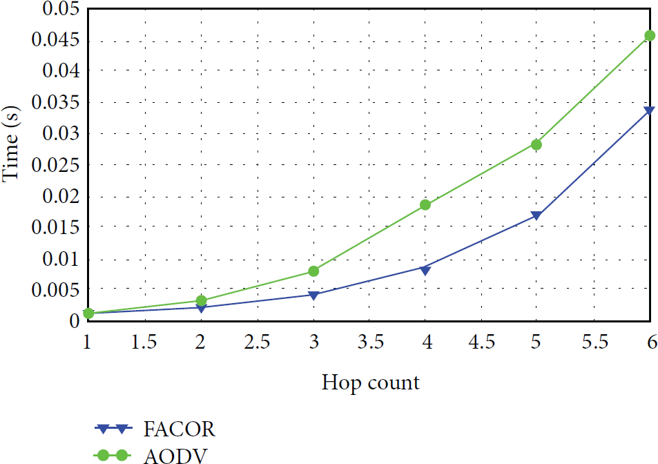
Figure 13 illustrates the routing setup time for FACOR and original AODV in the same scenario with the transmission range of 100 M for 10 nodes. In this figure, we are going to compare the routing setup time for two algorithms in different hop counts between the sender and receiver. As this figure shows, our proposed method is suitable for bigger hop count, to find the optimal path between sender and receiver; because of waiting time for arriving ants will take bigger time for routing. Of course, this parameter depends on the sender neighbor's number because we broadcast ants for all sender neighbors and whenever the number of ants is less, the routing setup time will be faster. In our simulation we did not control the sender neighbors.

Figure 13

Routing setup time.

4.3. Average End-to-End Delay

This is the average time taken by a data packet to travel from the source to the destination. It will be a different value with the routing setup time, because the routing path has been determined before and, by this field, we will only measure the time from the moment that a packet has been sent by sender until the moment that packet will be received by the receiver. The end-to-end delay is compared in Figure 14. This Figure depicts our algorithm, although it has a bigger routing setup time for finding optimal path, and when the path was determined, the optimal path of the end-to-end delay or the packet delivery time was better than the original AODV. Paying heed to this point, we can solve the increased routing setup time issue, because the energy will consume more when sending and receiving packets. As Figure 14 shows, the end-to-end delay time is approximately equal when the hop count is below 2. In this figure also, we assumed 10 nodes in a 100 M transmission range.

Figure 14

End-To-end delay.

4.4. Number of Packets

This field represents the amount of packets sent during the identification phase (RREQ packets). A low number of sent packets indicate that a protocol will be more efficient in terms of the energy spent during the route discovery. It is noteworthy that, due to this topic, ants in the first step (just for sender), the number of packets is extremely dependent on the sender neighbor's number. Also, this controls the amount of overhead on the network.

As we see in Figure 15, the number of packets for routing discovery in our proposal is the least. If the number of packets is the least, the amount of energy consumption will be lower. It is the number of packets since the discovery phase is started until ants find a route to the destination. Although the energy consumption amount for sending and receiving packet depends on the packet size and distance between the sender and receiver, our algorithm consumes the average of about 0.281 J for sending and receiving a packet. Also in Figure 15, we passed up the packets sent and received by broadcasting in our algorithm and original AODV.

Figure 15

The number of packets.

Finally, some anomalies in the figures are due to the fact that the nodes are randomly placed in the environment. Furthermore, when we have a transmission range equal to 100 M, each node in any distances in this transmission range is a neighbor and maybe sometimes one neighbor has 2 M distance and another has 99 M distance, but both of them are a neighbor for a given node.

5. Conclusion and Future Work

Due to some limitations in sensor nodes such as limited power battery source and some commonly used operations like routing, designing of optimal and efficient algorithm appears to be necessary. In this paper, we propose a novel optimal routing algorithm for WSN with fuzzy logic ant optimization colony routing called FACOR. Our proposed algorithm based on ant's intelligent optimization select the short path between the sender and receiver. Simulation results show the correct operation of the protocol and its suitability to be used in a wide range of applications and scenarios. The performance of this proposal has been compared with the original AODV. In this work, we calculated the routing setup time, end-to-end delay for packet delivery, and the number of packets sent in the routing discovery phase and energy consumption. Our algorithm increases the network lifetime by reducing the nodes energy consumption and the number of packets. Also FACOR has proven its efficiency by achieving better average results than the other proposals. Finding a solution for routing problems (e.g., nodes failure) and the addition of new nodes in the network is an open area for future work.

Footnotes

Conflict of Interests

The authors declare that there is no conflict of interests regarding the publication of this paper.

Acknowledgment

The authors would like to thank Professor Tien Van Do for the valuable and compassionate comments and guidance on doing this work.

References

Fernandez

P. M.

Circuit switching in the Internet [Ph.D. thesis] 2003

Stanford University

Frey

Rührup

Stojmenović

Routing in wireless sensor networks

Guide to Wireless Sensor Networks 2009

Berlin, Germany

Springer

81 111

Amiri

Keshavarz

Heidari

Mohamadi

Moradzadeh

Intrusion detection systems in MANET: a review

Proceedings of the International Conference on Innovation, Management and Technology Research

2013

Malacca, Malaysia

1 6

Keshavarz

Noor

R. M.

Mostajeran

Using routing table flag to improve performance of AODV routing protocol for VANETs environment

Proceedings of the 9th International Conference on Computing and Information Technology (IC2IT '13)

May 2013

73 82

10.1007/978-3-642-37371-8_11

Iwata

Chiang

C.-C.

Pei

Gerla

Chen

T.-W.

Scalable routing strategies for ad hoc wireless networks

IEEE Journal on Selected Areas in Communications 1999 17 8 1369 1379

2-s2.0-0032688633

10.1109/49.779920

Perkins

C. E.

Bhagwat

Highly dynamic destination-sequenced distance-vector routing (DSDV) for mobile computers

ACM SIGCOMM Computer Communication Review 1994 24 4 234 244

10.1145/190809.190336

Johnson

D. B.

Maltz

D. A.

Dynamic source routing in ad hoc wireless networks

Mobile Computing 1996

New York, NY, USA

Springer

153 181

10.1007/978-0-585-29603-6_5

Dorigo

Optimization, learning and natural algorithms [Ph.D. thesis] 1992

Milan, Italy

Politecnico di Milano

Colorni

Dorigo

Maniezzo

Distributed optimization by ant colonies

Proceedings of the 1st European Conference on Artificial Life

1991

134 142

10.

Zadeh

L. A.

Fuzzy sets

Information and Control 1965 8 3 338 353

2-s2.0-34248666540

11.

Zadeh

L. A.

The concept of a linguistic variable and its application to approximate reasoning—I

Information Sciences 1975 8 3 199 249

2-s2.0-0016458950

12.

Ghazanfari

Rezaei

G. M.

An Introduction to Fuzzy Sets Theory 2006

Tehran, Iran

Iran University of Science and Technology Press

13.

Ortiz

A. M.

Olivares

Fuzzy logic applied to decision making in wireless sensor networks

Fuzzy Logic—Emerging Technologies and Applications 221 240

10.5772/36430

14.

Ortiz

A. M.

Royo

Olivares

Castillo

J. C.

Orozco-Barbosa

Marron

P. J.

Fuzzy-logic based routing for dense wireless sensor networks

Telecommunication Systems 2013 52 4 2687 2697

2-s2.0-84879940783

10.1007/s11235-011-9597-y

15.

Sahani

S. K.

Kumar

Multi-routing in wireless sensor networks using an ant colony optimization (ACO)

International Journal of Computer Networking,Wireless and Mobile Communications 2013 3 3 87 98

16.

Suhonen

Kuorilehto

Hännikäinen

Hämäläinen

T. D.

Cost-aware dynamic routing protocol for wireless sensor networks—design and prototype experiments

Proceedings of the IEEE 17th International Symposium on Personal, Indoor and Mobile Radio Communications (PIMRC '06)

September 2006

Helsinki, Finland

1 5

2-s2.0-44949212192

10.1109/PIMRC.2006.254185

17.

Okdem

Karaboga

Routing in wireless sensor networks using an ant colony optimization (ACO) router chip

Sensors 2009 9 2 909 921

2-s2.0-63849162280

10.3390/s90200909

18.

Kadri

Feham

Mhammed

Efficient and secured ant routing algorithm for wireless sensor networks

International Journal of Network Security 2014 16 2 149 156

19.

Ghazizadeh

Zamani

Manan

J.-L. A.

Alizadeh

Trusted computing strengthens cloud authentication

The Scientific World Journal 2014 2014 17

260187

10.1155/2014/260187

20.

Alizadeh

Hassan

W. H.

Zamani

Karamizadeh

Ghazizadeh

Implementation and evaluation of lightweight encryption algorithms suitable for RFID

Journal of Next Generation Information Technology 2013 4 1 65 77

2-s2.0-84875427729

10.4156/jnit.vol4.issue1.9

21.

Cheng

An adaptive virtual area partition clustering routing protocol using ant colony optimization for wireless sensor networks

Advances in Wireless Sensor Networks 2014

Berlin, Germany

Springer

23 30

22.

Jafari

Khotanlou

A routing algorithm based an ant colony, local search and Fuzzy inference to improve energy consumption in wireless sensor networks

International Journal of Electrical and Computer Engineering 2013 3 640 650

23.

Chakraborty

Ganguly

Naskar

M. K.

Karmakar

A trust based congestion aware hybrid ant colony optimization algorithm for energy efficient routing in wireless sensor networks (TC-ACO)

http://arxiv.org/abs/1312.4077

24.

Correia

L. H. A.

Macedo

D. F.

dos Santos

A. L.

Loureiro

A. L.

Nogueira

J. M. S.

Transmission power control techniques in ad hoc networks

Guide to Wireless Sensor Networks 2009

Berlin, Germany

Springer

469 489

25.

Amiri

Keshavarz

Fahleyani

A. S.

Moradzadeh

Komaki

New algorithm for leader election in distributed WSN with software agents

Proceedings of the IEEE International Conference on Space Science and Communication (IconSpace '13)

July 2013

Melaka, Malaysian

290 295

10.1109/IconSpace.2013.6599483

26.

Akyildiz

I. F.

Sankarasubramaniam

Cayirci

A survey on sensor networks

IEEE Communications Magazine 2002 40 8 102 105

2-s2.0-0036688074

10.1109/MCOM.2002.1024422

27.

Abolfazli

Sanaei

Alizadeh

Gani

Xia

An experimental analysis on cloud-based mobile augmentation in mobile cloud computing

IEEE Transactions on Consumer Electronics 2014 60 1 146 154

10.1109/TCE.2014.6780937

28.

Zheng

Jamalipour

Wireless Sensor Networks: A Networking Perspective 2009

New York, NY, USA

John Wiley & Sons

29.

Chiasserini

Garetto

An analytical model for wireless sensor networks with sleeping nodes

IEEE Transactions on Mobile Computing 2006 5 12 1706 1718

2-s2.0-33750803950

10.1109/TMC.2006.175

30.

Battery-friendly packet transmission algorithms for wireless sensor networks

IEEE Sensors Journal 2013 13 10 3548 3557

2-s2.0-84883220153

10.1109/JSEN.2013.2276617

31.

Kailas

Brunelli

Weitnauer

M. A.

Comparison of energy update models for wireless sensor nodes with supercapacitors

Proceedings of the 1st International Workshop on Energy Neutral Sensing Systems (ENSSys '13)

2013

article 2

10.1145/2534208.2534223

32.

Heinzelman

W. B.

Chandrakasan

A. P.

Balakrishnan

An application-specific protocol architecture for wireless microsensor networks

IEEE Transactions on Wireless Communications 2002 1 4 660 670

2-s2.0-33646589837

10.1109/TWC.2002.804190

33.

Chakeres

I. D.

Belding-Royer

E. M.

AODV routing protocol implementation design

Proceedings of the 24th International Conference on Distributed Computing Systems Workshops

March 2004

698 703

2-s2.0-3042683156

34.

Perkins

C. E.

Royer

E. M.

Ad-hoc on-demand distance vector routing

Proceedings of the 2nd IEEE Workshop on Mobile Computing Systems and Applications (WMCSA '99)

February 1999

New Orleans, Louisiana

90 100

2-s2.0-34347349933

10.1109/MCSA.1999.749281

35.

Lin

X.-H.

Kwok

Y.-K.

Wang

Misra

S. C.

Woungang

Misra

Energy-efficient resource management techniques in wireless sensor networks

Guide to Wireless Sensor Networks 2009

London, UK

Springer

439 468

36.

Cheng

Xun

Zhou

An energy aware ant colony algorithm for the routing of wireless sensor networks

Intelligent Computing and Information Science 2011

Berlin, Germany

Springer

395 401 Communications in Computer and Information Science

10.1007/978-3-642-18129-0_62

37.

Amiri

Harounabadi

Mirabedini

Nodes clustering using Fuzzy logic to optimize energy consumption in Mobile Ad hoc Networks (MANET)

Management Science Letters 2012 2 8 3031 3040

10.5267/j.msl.2012.09.004

38.

Jang

J.-S. R.

Sun

C.-T. S.

Neuro-Fuzzy and Soft Computing: A Computational Approach to Learning and Machine Intelligence 1996

New York, NY, USA

Prentice-Hall

39.

Takagi

Sugeno

Fuzzy identification of systems and its applications to modeling and control

IEEE Transactions on Systems, Man and Cybernetics 1985 15 1 116 132

2-s2.0-0021892282

40.

Fall

Varadhan

The Ns Manual: The VINT Project 2001

Berkeley, Calif, USA

University of California, Berkeley

Energy Efficient Routing in Wireless Sensor Networks Based on Fuzzy Ant Colony Optimization

Abstract

1. Introduction

2. System Model and Problem Specification

2.1. Network Model and Assumptions

Assumption 1.

Assumption 2.

Assumption 3.

Assumption 4.

Assumption 5.

Assumption 6.

Assumption 7.

2.2. Sensor Nodes and Energy Consumption Model

2.2.1. Sensor Nodes Behavior

2.2.2. Energy Consumption Model

2.3. WSN Protocols and Improvements

2.3.1. AODV Routing Overview

2.3.2. MAC Layer

2.3.3. Traffic Protocol

2.3.4. Improvement in the Original AODV Routing

3. Proposed Solution

3.1. Ant Model and Fuzzy Logic Model

3.1.1. Energy Optimized Parameters

3.1.2. Linguistic Values and Membership Functions

3.2. Proposed Algorithm

Phase 1 (identification).

Pseudocode 1: Pseudocode for Step 1.

Pseudocode 2: Pseudocode for Step 2.

Pseudocode 3: Pseudocode for Step 3.

Phase 2 (relaxing).

Pseudocode 4: Pseudocode for Phase 2.

3.3. FACOR Sample

4. Simulation and Result

4.1. Energy Consumption

4.2. Routing Setup Time

4.3. Average End-to-End Delay

4.4. Number of Packets

5. Conclusion and Future Work

Footnotes

Conflict of Interests

Acknowledgment

References