Sage Journals: Discover world-class research

Abstract

A stabilized incompressible smoothed particle hydrodynamics (ISPH) method with the addition of a density invariant relaxation condition in the pressure calculations is applied to simulations of highly nonlinear liquid sloshing problems. By applying the Neumann boundary condition when solving pressure, the performance of the present ISPH method is enhanced significantly. Two large-amplitude free sloshing problems under a resonance sway excitation were carried out in a square and a rectangular tank with filling-depths ratios of 20% and 50% of tank height, respectively, and compared with the available published experimental results. To extend the validation of the method, numerical simulations for sloshing problems with the varying density of a floating body as well as a middle baffle, which also generates strongly nonlinear free surface flow, were conducted. The results showed that the present ISPH method produces smooth pressure distribution and significantly reduces spurious oscillation. The proposed ISPH method was shown to be robust and accurate in long time simulation of highly nonlinear sloshing problems.

1. Introduction

Sloshing refers to the liquid motion within a partially filled container due to external excitations. At special critical conditions, such as significant container motion or occurrence of resonance at which the excitation frequency is close to the natural frequency of the liquid sloshing system, the liquid can experience violent oscillations. Consequently, the induced strong impact pressure causes significant structural load on the container structure [1]. These sloshing phenomena can frequently be found in a wide range of engineering applications, such as the liquefied natural gas (LNG) carrier, a ship under the effect of ocean waves, a reservoir during an earthquake, and an automotive and an aircraft fuel tank. Due to the crucial effect of sloshing on the tank structure, an accurate prediction of liquid sloshing behavior is essential for tank design [2, 3].

During the past few decades, interest in sloshing phenomenon has grown and many studies have been conducted using various techniques including theoretical, experimental, and numerical methods. It is evident that theoretical studies are suitable for dealing with linear or weakly nonlinear liquid sloshing dynamics and are in general not able to solve more complex sloshing motions. Experimental work is practical for studying the physics of sloshing although it has limitations by high cost and requirement of a high level of accuracy. Numerical techniques have provided an alternative method for studying highly nonlinear sloshing problems. Detailed reviews of numerical methods for liquid sloshing problems can be found in many studies [4 –7]. During the last decade, numerical studies primarily employed grid-based methods, such as the finite difference method (FDM) [8, 9], finite element method (FEM) [10, 11], and boundary element method (BEM) [12 –15]. The conventional grid-based method encounters many difficulties involving the discontinuity of liquid motion or breaking waves. While some free-surface tracking techniques such as the volume-of-fluid (VOF) [16, 17] and level set [18] were introduced to overcome these drawbacks and improved the performance of conventional mesh-based methods, they still cannot handle large fluid deformation, and as such mesh adjustment or rezoning is necessary to resolve liquid sloshing phenomena.

Recently, mesh-free and particle methods have been developed, and have gradually become alternative techniques for analyzing nonlinear free surface flows [19 –21]. The smoothed particle hydrodynamics (SPH) is one of the meshless methods originally developed for solving compressible flow, and then some special treatment was applied to enforce the incompressible condition [21]. In the incompressible SPH method, the pressure is implicitly calculated by solving a discretized pressure Poisson equation (PPE) at every time step. Lee et al. [22] demonstrated that the incompressible SPH model is able to realistically predict the pressure field of the flows based on the hydrodynamic formulations. Gómez-Gesteira et al. [23], Shao [24], and Cleary and Rudman [25] employed the incompressible SPH method for determining both oceanic and offshore hydrodynamics. The incompressible SPH model has recently been applied to simulate the industrial and environmental flows associated with incompressible free-surface fluids [26 –33]. It was also used to simulate the highly nonlinear two-dimensional sloshing phenomenon, as in the studies of Souto-Iglesias et al. [34], Rafiee et al. [35], Marsh et al. [36], and Shao et al. [37]. In a continuing attempt to improve handling incompressible fluids, Lee et al. [27] presented comparisons between the semi-implicit and truly incompressible SPH algorithms with the classical, weakly compressible SPH method. They demonstrated that problems encountered in weakly compressible SPH when solving incompressible flows could be resolved by using an incompressible SPH scheme. Khayyer et al. [28, 29] also proposed a corrected incompressible SPH method, which was developed, based on a variational approach to ensure the angular momentum conservation of incompressible SPH formulations. Recently, a stabilized incompressible SPH method involving relaxation of the density invariance condition was proposed by Asai et al. [31]. In this technique, the PPE was solved in relation to velocity divergence-free and density invariance conditions. This formulation leads to a new PPE with a relaxation coefficient, which can be estimated via a preanalysis calculation. Asai et al. [31] tested the efficiency of the proposed formulation via a numerically modeled dam-breaking problem, and discussed its effects using several resolution models with different initial particle distances.

Aly et al. [32] modeled the surface tension force and an eddy viscosity based on the Smagorinsky subgrid scale model for free surface flows using incompressible SPH method. They demonstrated that the eddy viscosity has clear effects in adjusting the splashes and reduces the deformation of free surface in the interaction between two fluids. It was also exhibited that the proposed stabilization by the relaxation of density invariance with velocity divergence in PPE has an important role to preserve the total volume of fluid by decreasing particles clustering. In addition, Aly et al. [33] applied the stabilized incompressible SPH method to simulate free falling of rigid body and water entry/exit of circular cylinder into water tank.

In the most recent work by Koh et al. [38], the consistent particle method was proposed to eliminate pressure fluctuation in solving large-amplitude, free-surface motion. In this method, a zero-density-variation condition and a velocity-divergence-free condition were also combined in a source term of PPE to enforce fluid incompressibility. Aly and Lee [39] adapted incompressible SPH method to simulate impact flows associated with complex free surface. They tested the accuracy and efficiency of the proposed incompressible SPH method using several typical problems with largely distorted free surface, including 2D dam-break over horizontal and inclined planes with different inclination angles, as well as the water entry of a circular cylinder into a tank. Lishi et al. [40] applied the SPH method to simulate the large-amplitude lateral sloshing both with and without a floating body and the parametrically excited sloshing in a 2D tank. They showed that the SPH approach has an obvious advantage over conventional mesh-based methods in handling nonlinear sloshing problems such as violent fluid-solid interaction, flow separation, and wave-breaking on the free fluid surface. Ozbulut et al. [41] introduced a series of numerical treatments to refine the numerical procedures of the SPH method, particularly, for violent flows with a free surface. They modeled 2D dam-break and sway-sloshing problems in a tank by solving Euler's equation of motion utilizing weakly compressible SPH method. Chen et al. [42] investigated the pressure on solid boundaries in 2D sloshing problem for forced rolling motion using SPH method. They combined some advanced correction algorithms in SPH method. The moving least squares (MLS) method was used in the density reinitialization to obtain smoother and more stable pressure field in numerical simulation. Gotoh et al. [43] presented two schemes for enhancement of incompressible SPH based methods in simulation of violent sloshing flows, and, in particular, sloshing induced impact pressures. The enhanced schemes include a higher order Laplacian and an error-compensating source of PPE.

The present study introduces an incompressible SPH method based on the previous studies of the same author [31 –33], in which velocity-divergence free and density invariance are contributed as the source term of the PPE. The present scheme imposes the Neumann boundary condition for pressure, as opposed to the Dirichlet boundary condition in the previous works, which consider zero pressure on the free surface for both fluid and boundary particles. To demonstrate the improvement by this alternative pressure boundary condition, large-amplitude, rectangular tank sloshing problems with various filling-depth ratios under a resonance sway excitation were numerically solved and compared with the available experimental data. The results showed that the present incompressible SPH scheme creates smooth pressure distribution with significantly reduced spurious oscillation and is more robust and accurate in long-period simulations of nonlinear sloshing.

2. Model Description

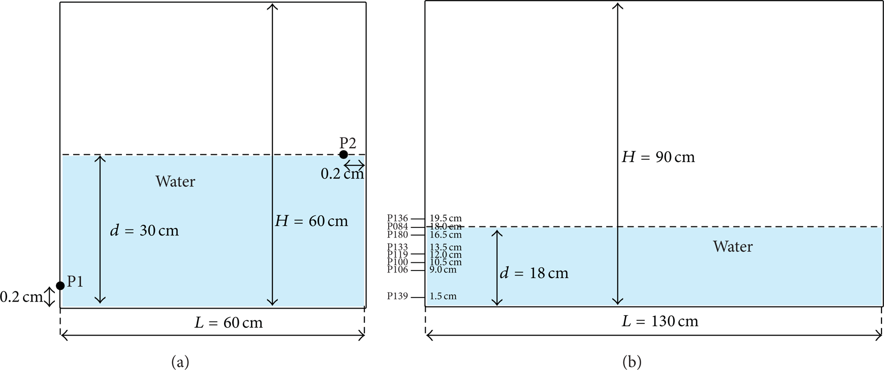
Various computational set-ups were investigated to validate and examine the performance of the incompressible SPH algorithm with two different pressure boundary conditions. The schematic views of four models of liquid sloshing in a rectangular and a square tank under the translation excitation are shown in Figures 1 and 2. According to the experimental work of Koh et al. [38], the first sloshing configuration as shown in Figure 1(a) was considered with a relatively high ratio of filling depth (d = 0.5H). The excitation frequency ω was chosen to be the same as the fundamental frequency ω₀ of the natural frequency of the sloshing system. This leads to resonance, which is believed to stimulate the violent sloshing motion. In this model, the fundamental frequency of the natural frequency for a square tank is obtained as ω₀ = 6.85 rad/s by linear theory [43]. Thus, sloshing was induced by an excitation motion, x = A(1 − cos ⁡ ⁡ ωt), where the amplitude, A, is 0.005 m, and the excitation frequency is ω = ω₀.

Figure 1:

Schematic diagram of the two free liquid sloshing models: (a) model 1 corresponding to Koh et al. [38] and (b) model 2 corresponding to Rafiee et al. [35].

Figure 2:

Schematic diagrams of sloshing models (a) with a floating rigid body, (b) with middle baffle.

The second model was constructed based on the experimental work of Rafiee et al. [35], with a low ratio of filling depth (d = 0.2H) and an excitation of sinusoidal motion, x = Asin ⁡ ωt. Here, the large amplitude of the motion (A = 0.1 m) and resonance frequency, ω = 3.116 rad/s, were applied. Detailed dimensions of the rectangular tank in this model are described in Figure 1(b).

The schematic diagram for the motion of a free rigid body over sloshing water in a tank introduced in Figure 2(a) is similar to Koh et al.'s work [38]. The floating rigid body is a 2D rectangular block, H = 0.26 m in length and L = 0.03 m in height. The water depth is d = 0.5H. In order to investigate the motion of a free rigid body inside a sloshing tank, three different density ratios, β = ρ_s/ρ_f = 0.52, 1.0 and 1.25 were considered, where ρ_s and ρ_f are the density of the rigid body and water, respectively. The sloshing of the water was induced by a sinusoidal displacement, x = Asin ⁡ ωt, where the excitation amplitude is A = 0.004 m, and the frequency ω = 7.4 rad/s. Figure 2(b) shows another example for water sloshing in a square tank with a middle baffle. The dimensions of the tank and excitation motion are the same as those of the sloshing model with a floating rigid body, but with the existence of a baffle of 0.15 m in height at the middle of the bottom wall.

3. Incompressible SPH Formulation

The incompressible SPH formulation is a procedure similar to the moving particle, semi-implicit method (MPS) proposed by Koshizuka et al. [21]. The primary feature is the application of a semi-implicit integration scheme to particle-discretized equations for the incompressible flow problem.

3.1. Governing Equation

The mass and momentum conservation equations are presented as

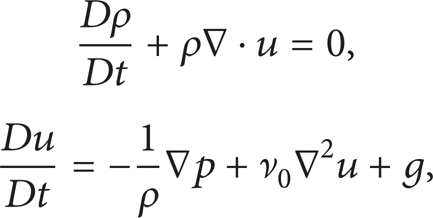
\begin{matrix} \frac{D ρ}{D t} + ρ \nabla \cdot u = 0, \\ \frac{D u}{D t} = - \frac{1}{ρ} \nabla p + ν_{0} \nabla^{2} u + g, \end{matrix}

(1)

where ρ and ν₀ are the density and kinematic viscosity of the fluid, u and p are the velocity vector and pressure of the fluid, respectively, and t indicates time. In the most general incompressible flow approach, the density ρ, is assumed by a constant value, ρ⁰, with the initial value. The aforementioned governing equations lead to the following progression as follows:

\begin{matrix} \nabla \cdot u = 0, \\ \frac{D u}{D t} = - \frac{1}{ρ^{0}} \nabla p + ν_{0} \nabla^{2} u + g . \end{matrix}

(2)

The primary issue in an incompressible SPH method is solving a discretized PPE at every time step to obtain the pressure field. In this study, the following formulation is mathematically derived and used for pressure calculation:

〈\nabla^{2} p^{n + 1}〉 = \frac{ρ^{0}}{Δ t} 〈\nabla \cdot u^{*}〉 + α \frac{ρ^{0} - 〈ρ^{n}〉}{Δ t^{2}},

(3)

where (0 ≤ α ≤ 1) is the relaxation coefficient, u^* the temporal velocity, and the triangle bracket 〈〉 is the SPH approximation. A detailed procedure for deriving (3) can be found in Asai et al. [31].

3.2. SPH Formulation

The fundamental basis of the SPH method is the interpolation theory. The method allows any function to be expressed in terms of its values at a set of disordered points representing particle positions using the kernel function. A physical scalar function A(r) at a specific position, r, can be represented by the following integral form:

A (r) = \int_{V}^{} A (r^{'}) W (r - r^{'}, h) d r^{'},

(4)

where V represents the solution space, and the smoothing length, h, represents the effective width of the kernel. The properties of the kernel function should satisfy the following two conditions for mass and energy conservation:

\int_{V}^{} W (r - r^{'}, h) d r^{'} = 1, \lim_{h \to 0} W (r - r^{'}, h) = δ (r - r^{'}) .

(5)

For SPH numerical analysis, the integral in (4) is approximated by a summation of contributions from neighbor particles in the support domain:

A (r_{i}) \approx 〈A_{i}〉 = \sum_{j} \frac{m_{j}}{ρ_{j}} W (r_{i j}, h) A_{j} (r_{j}, t),

(6)

where the subscripts i and j indicate the positions of a labeled particle, and m_j is the representative mass related to particle j. The density 〈ρ_iⁿ〉 in SPH form is defined by

ρ (x_{i}) \approx 〈ρ_{i}〉 = \sum_{j} m_{j} W (r_{i j}, h) = \sum_{j} m_{j} W_{i j} .

(7)

The gradient of the scalar function can be obtained via the defined SPH approximation, as follows:

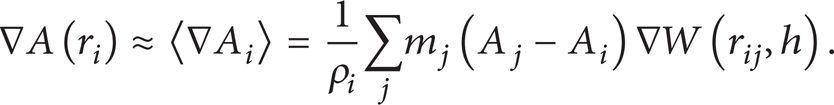
\nabla A (r_{i}) \approx 〈\nabla A_{i}〉 = \frac{1}{ρ_{i}} \sum_{j} m_{j} (A_{j} - A_{i}) \nabla W (r_{i j}, h) .

(8)

The other expression for the gradient can be represented by

\nabla A (r_{i}) \approx 〈\nabla A_{i}〉 = ρ_{i} \sum_{j} m_{j} (\frac{A_{j}}{ρ_{j}^{2}} + \frac{A_{i}}{ρ_{i}^{2}}) \nabla W (r_{i j}, h) .

(9)

The quintic spline function is utilized as a kernel function. Consider

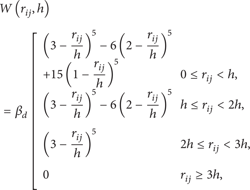
W (r_{i j}, h) = β_{d} [\begin{matrix} {(3 - \frac{r_{i j}}{h})}^{5} - 6 {(2 - \frac{r_{i j}}{h})}^{5} \\ + 15 {(1 - \frac{r_{i j}}{h})}^{5} & 0 \leq r_{i j} < h, \\ {(3 - \frac{r_{i j}}{h})}^{5} - 6 {(2 - \frac{r_{i j}}{h})}^{5} & h \leq r_{i j} < 2 h, \\ {(3 - \frac{r_{i j}}{h})}^{5} & 2 h \leq r_{i j} < 3 h, \\ 0 & r_{i j} \geq 3 h, \end{matrix}

(10)

where β_d is 7/478πh² and 3/358πh³, respectively, in two- and three-dimensional spaces. In the present incompressible SPH method, the gradient of pressure and divergence of velocity are approximated as follows:

\nabla p (r_{i}) \approx 〈\nabla p_{i}〉 = ρ_{i} \sum_{j} m_{j} (\frac{p_{j}}{ρ_{j}^{2}} + \frac{p_{i}}{ρ_{i}^{2}}) \nabla W (r_{i j}, h),

(11)

\nabla \cdot u (r_{i}) \approx 〈\nabla \cdot u_{i}〉 = ρ_{i} \sum_{j} m_{j} (u_{j} - u_{i}) \cdot \nabla W (r_{i j}, h) .

(12)

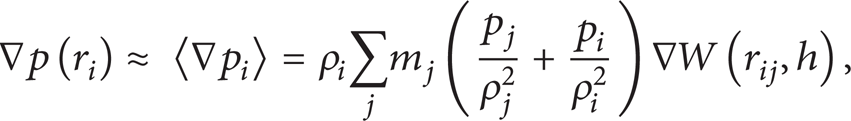
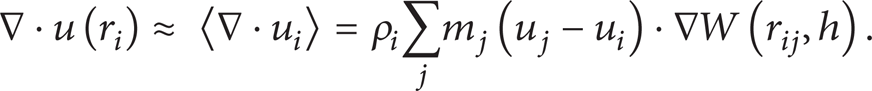
Although the Laplacian could be derived directly from the original SPH approximation of a function in (11), this approach may lead to a loss of resolution. The second-order approximation proposed by Lishi et al. [40] is utilized for the Laplacian terms in this study. Consider

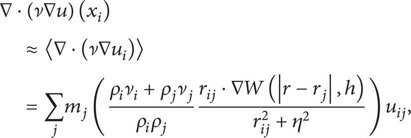
\nabla \cdot (ν \nabla u) (x_{i}) \approx 〈\nabla \cdot (ν \nabla u_{i})〉 = \sum_{j} m_{j} (\frac{ρ_{i} ν_{i} + ρ_{j} ν_{j}}{ρ_{i} ρ_{j}} \frac{r_{i j} \cdot \nabla W (|r - r_{j}|, h)}{r_{i j}^{2} + η^{2}}) u_{i j},

(13)

where η is a parameter to avoid a zero denominator and its value is usually given as η² = 0.0001h². For the case of ν_i = ν_j and ρ_i = ρ_j, the Laplacian term is simplified as

\nabla \cdot (ν \nabla u) (x_{i}) = \frac{2 ν_{i}}{ρ_{i}} \sum_{j} m_{j} (\frac{r_{i j} \cdot \nabla W (|r - r_{j}|, h)}{r_{i j}^{2} + η^{2}}) u_{i j} .

(14)

Similarly, the Laplacian of pressure in the PPE is given by

\nabla^{2} p (x_{i}) = 〈\nabla^{2} p_{i}〉 = \frac{2}{ρ_{i}} \sum_{j} m_{j} (\frac{p_{i j} r_{i j} \cdot \nabla W (|r - r_{j}|, h)}{r_{i j}^{2} + η^{2}}) .

(15)

The PPE after SPH interpolation is solved by a preconditioned (diagonal scaling) conjugate gradient (PCG) method with a convergence tolerance (= 1.0 × 10^{− 9}).

4. Treatment of a Moving Rigid Body

Koshizuka et al. [21] proposed a passively moving solid model to describe the motion of a rigid body in a fluid. According to this study, the treatment of the moving rigid body in the fluid can be divided into two steps. First, both the fluid and solid particles are solved via the same calculation procedures. Secondly, an additional procedure is applied to solid particles.

Considering n solid particles with location, r_k, the center of the solid object, r_c, and the relative coordinate of a solid particle to the center, q_k, the moment of inertia, I, of the rigid body can be calculated as follows:

\begin{matrix} r_{c} = \frac{1}{n} \sum_{k = 1}^{n} r_{k}, \\ q_{k} = r_{k} - r_{c}, \\ I = \sum_{k = 1}^{n} {|q_{k}|}^{2} . \end{matrix}

(16)

The translational velocity, T, and rotational velocity, R, of a rigid body are calculated as follows

\begin{matrix} T = \frac{1}{n} \sum_{k = 1}^{n} u_{k}, \\ R = \frac{1}{I} \sum_{k = 1}^{n} u_{k} \times q_{k} . \end{matrix}

(17)

Finally, the velocity of each particle in the solid body can be expressed as

u_{k} = T + q_{k} \times R .

(18)

Gotoh and Sakai [44] and Shao [45] showed that the above treatment can be applied to a free-falling wedge in water and works well in a stable computation where the Courant condition is satisfied.

5. Treatment of the Boundary Condition

The boundary condition plays an important role in preventing penetration and reducing truncation error in the kernel function. In order to prevent penetration in the present study, we implemented a dummy boundary particles technique, in which dummy particles are regularly distributed at the initial state with zero velocity [27]. For the PPE of (3), two different pressure boundary conditions are implemented at dummy boundary particles, which are Neumann (∂p/∂n = 0) (C1) and Dirichlet boundary condition (p = 0) (C2). For Neumann boundary condition, the summation of the source term on the right side of the PPE of (3) after discretization is equal to zero for all dummy boundary particles.

On the free surface, Dirichlet boundary condition (C2) was imposed by considering the zero pressure (p = 0) as in previous works [21, 31 –38]. Here, we solved PPE for the entire domain, including dummy boundary particles.

6. Results and Discussion

6.1. Liquid Sloshing in a Square and a Rectangular Tank

Figure 3 presents free surface wave profiles with the pressure distribution at several time instants for the sloshing in a square tank as shown in Figure 1(a). The pressure distribution is smooth and exhibits a good trend throughout the computational domain with imposing the Neumann boundary condition for pressure (C1). The pressure appears to be at zero on the wave surface and becomes greater with increasing water depth. The greatest values of pressure can be obtained near the corner connecting the bottom wall to the side wall (point P1) being hit by a wave of water (t = 7.5 s). It is observed that following the origination of the excitation motion, a standing wave is formed in the tank (t = 0.1 s). The free surface subsequently becomes higher with time, and a nonlinear sloshing wave with a sharp wave crest and trough is consequently observed (t = 9.0 s). It can be seen that with the current model set-up (Figure 1(a)), there is no breaking or traveling wave occurrence. The water wave continues to increase in height after hitting the side walls until a steady state is reached.

Figure 3:

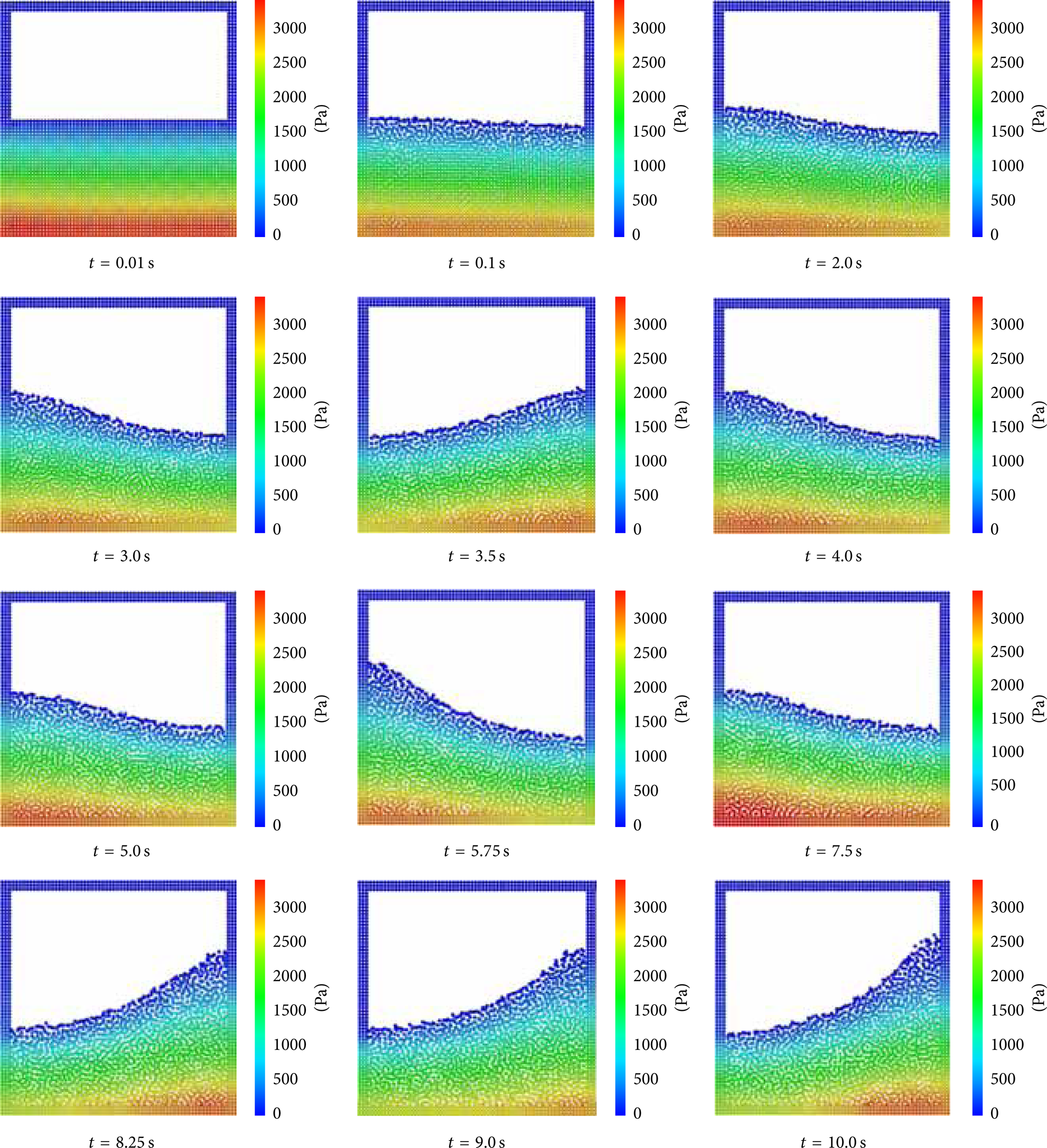
Snapshots of the pressure distributions for liquid sloshing with a high filling depth (d = 0.5H), corresponding to Koh et al. [38].

In order to demonstrate the advantage of the Neumann pressure boundary condition, comparisons of time histories of pressure at point P1 and the water elevation at point P2 with the results via Dirichlet pressure boundary condition and the experimental data [28] are shown in Figure 4. The results obtained via the Neumann pressure boundary condition (C1) exhibit significantly better agreement with the experimental data when compared to those achieved via the Dirichlet condition (C2), even for low particle resolution (d₀ = 0.01 m). Using the same particle size d₀ = 0.01 m, Dirichlet pressure boundary condition (C2) leads to significantly lower pressure values when compared to the experimental data. While an increase of the number of particles (a reduction in particle size to d₀ = 0.005 m) may improve the accuracy of pressure, it raises the issue of computer memory and computational time consumption when dealing with the large system of particles. Hence, imposing the Neumann boundary condition for pressure provides great benefit in terms of accuracy as well as saving memory. We observed that the pressure from case C1 shows less fluctuations and two clear sharp pressure peaks that are in excellent agreement with the experimental data; whereas for case C2, even with high resolution (d₀ = 0.005 m), the pressure at point P1 shows more oscillation from the initial time, and the two unequal pressure peaks are not comparable with those of the experimental results. Similar trends were observed in the wave elevation shown in Figure 4(b). Although the temporal variations in water height with both pressure boundary conditions are generally comparable with the experimental values, the peak wave height values in case C2, even at d₀ = 0.005 m are still lower than the experimental results. The maximum water height from case C1 is a better fit to experimental data.

Figure 4:

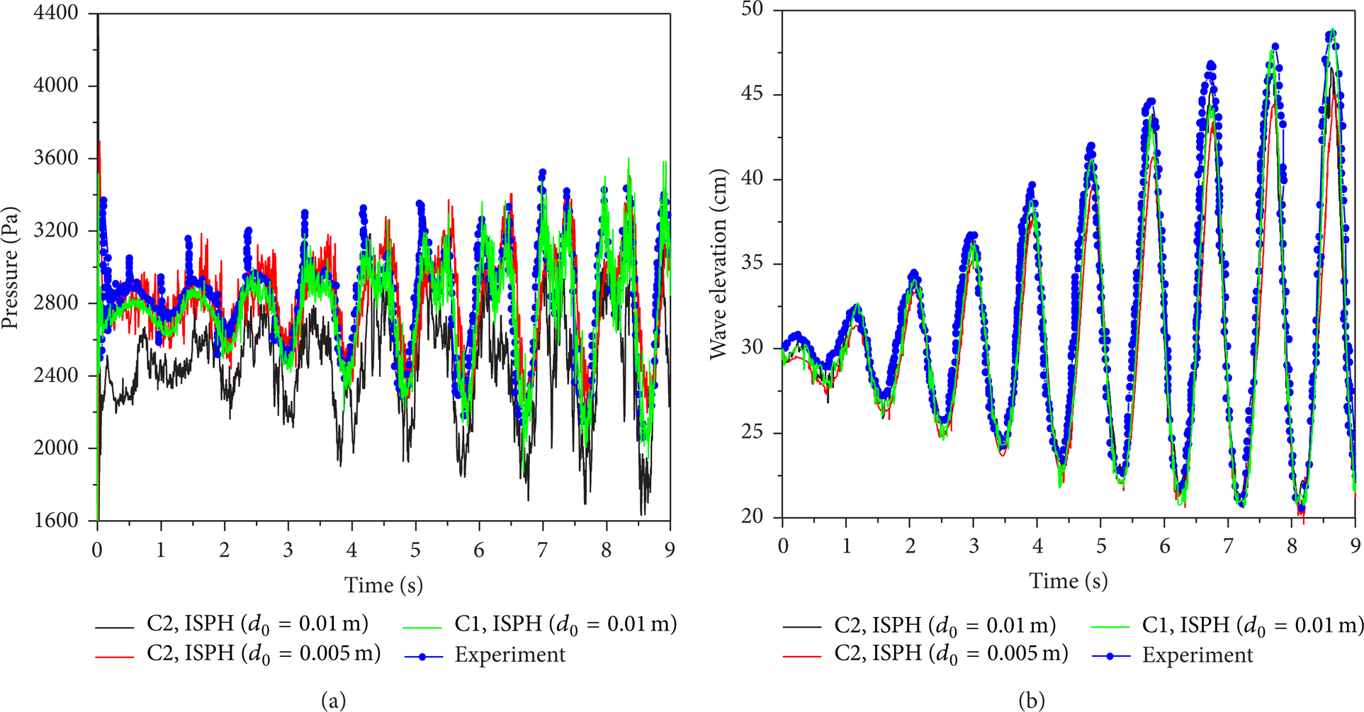
A comparison of time histories for cases C1 and C2 and the available experimental data [38] (a) the pressure distributions at P1, (b) the water elevation at P2.

Figure 5 presents snapshots of the pressure distributions for a liquid sloshing model in a rectangular tank (shown in Figure 1(b)) which corresponds to the experimental work of Rafiee et al. [35]. The low filling depth (d = 0.2H) and greater longitudinal tank motion (A = 0.1 m) at the resonance frequency, evidently lead to different sloshing behavior compared to in the first model (refer to Figure 3). After the origination of the external excitation, the standing wave rapidly changes into traveling waves with a wave crest (t = 0.5 s). The travelling wave subsequently hits the left wall of the tank (t = 1.3 s), returns, and forms sharper crest waves before hitting the right wall (t = 1.8 s). The wave then falls back and results in the formation of a bore (t = 2.2). The high elevation wave surface again travels in the tank (t = 2.5 s) and eventually hits the left wall (t = 2.8). The water then climbs up along the left wall, breaks the wave and impacts on the wall. The breaking wave falls back to the remaining water body and continues traveling until steady state is reached. The long time behavior of pressure distribution at several time instants (untilt = 85 s) can also be observed in Figure 5. It is noticed that imposing the Neumann boundary condition for pressure (C1) leads to reasonable pressure results, whereas Dirichlet boundary condition (C2) leads to poor performance of water sloshing or even diverging. Here, due to long time simulation of wave sloshing with impacts the wall (untilt = 85 s), small discontinuities happen between the fluid and the wall and such discontinuities may be eliminated by introducing turbulence model and improving boundary treatments.

Figure 5:

Snapshots of the pressure distributions for liquid sloshing with a low filling depth (d = 0.2H), corresponding to Rafiee et al. [35].

The comparison of impact pressures at points P119 and P136 between the present incompressible SPH method (with Neumann pressure boundary condition, C1) and the experimental results [35] is presented in Figure 6. It is clear that numerical results are in good agreement with experimental data. Throughout two incompressible SPH simulations for highly nonlinear sloshing with varied filling depth and excitation magnitude at resonance frequency, we confirmed the superiority of the Neumann pressure boundary condition (C1) over Dirichlet (C2) which were imposed in previous studies [31 –33] in respect of accuracy and robustness. It can be found in Figures 5 and 6 that the rolling and breaking waves appear on the free surface. For these distorted deformation and discontinuous cases, the conventional mesh-based methods often lead to overflow and stop the calculation process. This example indicates the advantage of the ISPH over the mesh-based methods in predicting the nonlinear sloshing motion.

Figure 6:

A comparison of the impact pressure between the present incompressible SPH method and the experimental results [35] at (a) P119, (b) P136.

6.2. Liquid Sloshing with a Freely Floating Rigid Body and a Middle Baffle

The sloshing with a floating body can be frequently observed in hydraulic engineering, such as the ship-lifter system, and ship and water way (or aqueduct bridge) system. In these systems, the floating body (immersed ship) can be treated as a rigid (floating) body.

In order to demonstrate the applicability of the present incompressible SPH method to the modelling of the rigid body motion in sloshing, we carried out numerical simulations of liquid sloshing with a freely floating rigid body as well as a middle baffle.

Figure 7 shows the snapshots of free sloshing and sloshing with a freely floating body of the solid-fluid density ratio (β = 0.52) and a middle baffle at three different time points. It can be visually observed that the addition of a baffle at the middle of the bottom wall of the tank clearly reduces the wave height of the free surface, whereas the existence of floating body does not strongly affect the behavior of the sloshing liquid. This is more clearly seen by considering the temporal pressure variation at point P3 and water height at point P4 for the three cases as shown in Figure 8. Despite the similar behavior of pressure and water height for the three models at the initial state, after t = 2 s, the addition of a middle baffle yielded a significant reduction in the pressure at point P3 (15% reduction) and the free surface motion (28% reduction) when compared with those of the free sloshing problem. This addition, therefore, results in the suppression of the impact load onto the tank. It is clearly observed in Figure 8 that the pressure value and wave elevation of the free sloshing and the sloshing with a floating rigid body are similar throughout the simulation.

Figure 7:

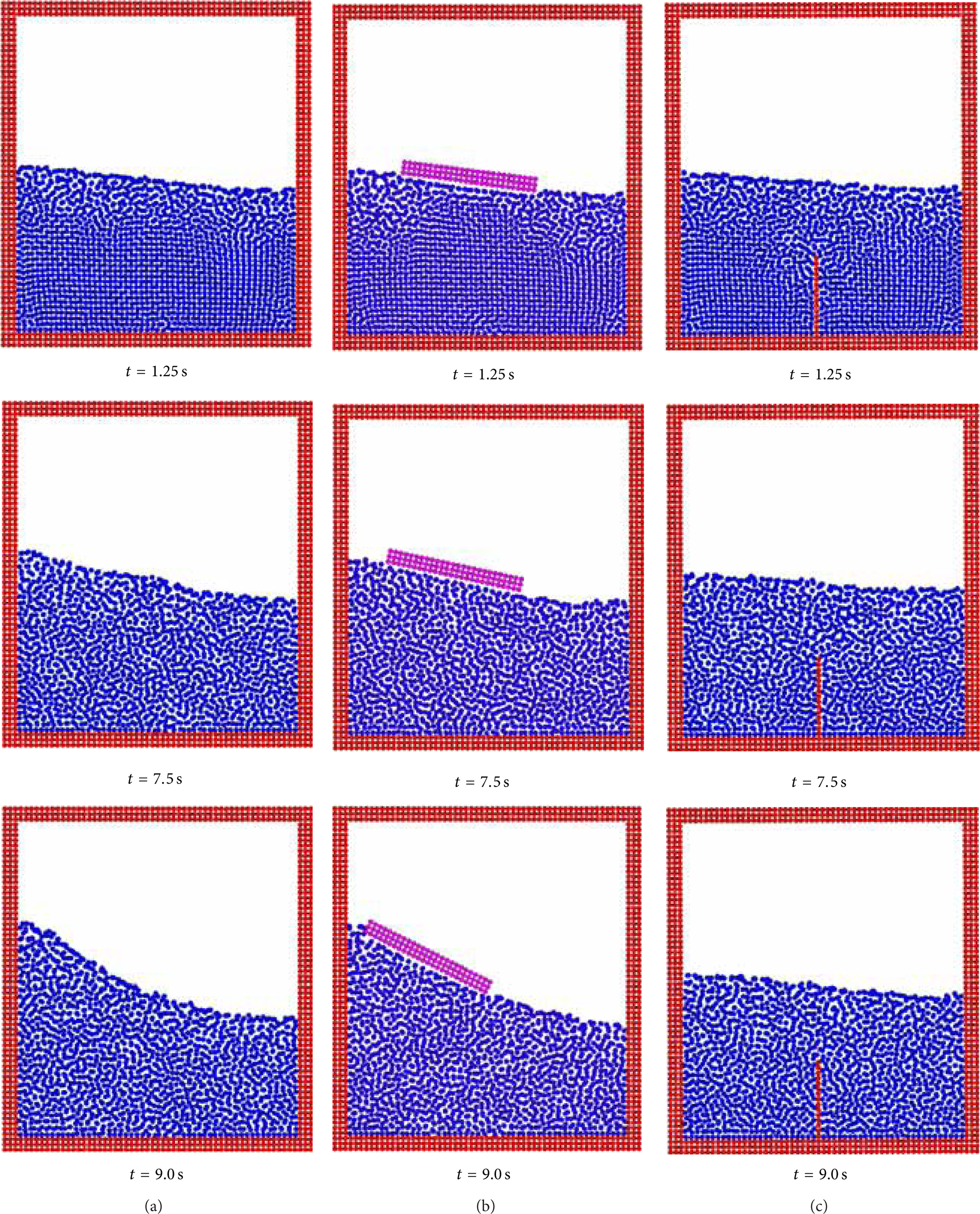
Snapshots of liquid sloshing: (a) free sloshing, (b) with a freely floating rigid body, (c) with a middle baffle.

Figure 8:

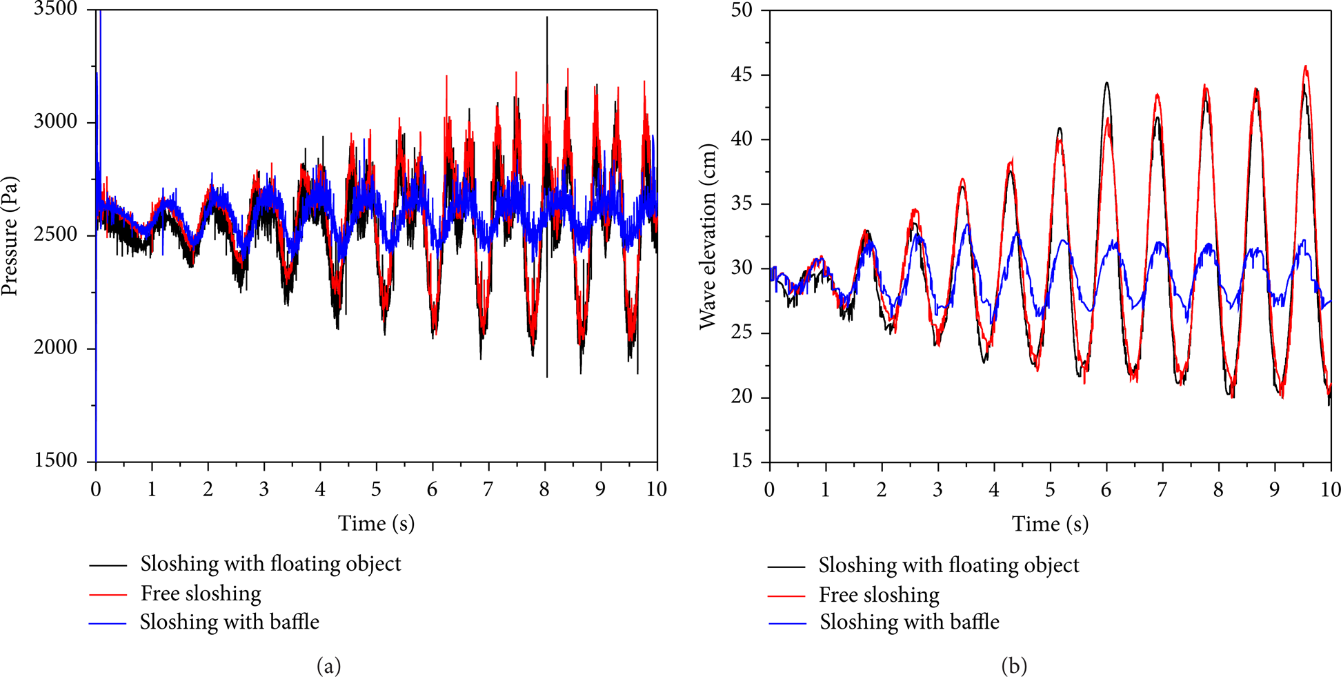
A comparison of time histories for three different cases: sloshing with a floating body, free sloshing, and sloshing with a middle baffle: (a) pressure at point P3 and (b) water elevation at point P4.

The effect of the density ratio β between the rigid body and the liquid on the rigid body motion in sloshing was investigated by considering three different density ratios β = 0.52, 1.0 and 1.25. The initial position of rigid body was the middle of the free surface as shown in Figure 2(a). As the external excitation is applied, the rigid body moves freely inside the tank (Figure 9). It is clear that for β = 0.52, the rigid body floats harmoniously over the free surface for the duration of the simulation. As the density of the rigid body resembles the one of the water β = 1.0, the rigid body initially floats over and travels with the free surface wave (t = 0.5 s, 1.5 s). As the water wave hits the wall and falls down over the moving rigid body (t = 3.0 s), the rigid body dives below the free surface and travels inside the water. The force applied by the moving fluid continues to drag the rigid body until it hits the wall and consequently pulses back (t = 9.5 s). Contrary to the two previous cases, in the case of the massive body (β = 1.25), the rigid body rapidly falls down and touches the bottom wall about two seconds following the application of the excitation motion. Due to the pressure force of the sloshing water, the rigid body continues to fluctuate back and forth on the bottom wall surface (t = 2.5 s~9.5 s).

Figure 9:

The motion of a freely floating rigid body with density ratios β = 0.52, 1.0 and 1.25 in a sloshing tank.

Figure 10 shows time histories for the pressure and free surface elevation at different density ratios between the rigid body and the liquid. It can be observed in Figure 10(a) that for the case of a high density ratio (β = 1.25), the oscillation in pressure occurs during the time of the rigid body falling down to the tank bottom (t = 1.75~2.25 s). After steady state is established, oscillations reduce and the typical pressure variation is obtained with two sharp pressure peaks where the surface wave hits the wall and the overturned wave falls hitting the remaining body of water. For the case of β = 0.52 and 1.0, the same trend of pressure variation is obtained with the exception that no severe oscillations occur during initial state. Figure 10(b) shows the comparison of free surface elevation at point P4 for three different cases of ratio β. It can be seen that the temporal variation of free surface elevation are similar and the average values which are shifted slightly up as the density of the rigid body increases. An increase in the average water height as density ratio β becomes higher can be interpreted by an increase in water volume as the rigid body sinks completely into the body of water. In addition, in the case β = 0.52, the floating body occupies and makes the free surface more “stiff.” The rigid body therefore can be considered to have only minor damping effect on sloshing.

Figure 10:

Time histories of sloshing with rigid bodies of different density: (a) pressure at point P3 and (b) free surface elevation at point P4.

7. Conclusion

An incompressible SPH model with an alternative Neumann pressure boundary condition is successfully adapted to investigate large-amplitude free sloshing problems with different ratios of filling depth (20% and 50% of tank height) in a square and a rectangular tank under resonant sway excitation. Results were then compared with available experimental data and showed good agreement. Moreover, a comparison of Neumann and Dirichlet boundary conditions for pressure revealed that great improvement of the accuracy in long time simulations of highly nonlinear sloshing problems could be achieved.

In addition, numerical simulations of the liquid sloshing with freely floating bodies of varying density and a middle baffle demonstrated that a middle baffle leads to significant reduction in the water height and therefore suppresses the impact pressure on the tank wall, but that a floating body has only minor effect on the water wave elevation.

Conflict of Interests

The authors declare that there is no conflict of interests regarding the publication of this paper.

Footnotes

Acknowledgment

This work was supported by 2013 Special Research fund of Mechanical Engineering at the University of Ulsan.

References

Ibrahim

R. A.

, Liquid Sloshing Dynamics-Theory and Applications, Cambridge University Press, Cambridge, UK, 2005.

Akyildiz

and Ünal

, “Experimental investigation of pressure distribution on a rectangular tank due to the liquid sloshing,” Ocean Engineering, vol.32, no. 11–12, pp. 1503–1516, 2005.

Kim

Shin

Y.-S.

, and Lee

K. H.

, “Numerical study on slosh-induced impact pressures on three-dimensional prismatic tanks,” Applied Ocean Research, vol. 26, no. 5, pp. 213–226, 2004.

Kleefsman

K. M.

Fekken

Veldman

A. E.

Iwanowski

, and Buchner

, “A volume-of-fluid based simulation method for wave impact problems,” Journal of Computational Physics, vol. 206, no. 1, pp. 363–393, 2005.

Ibrahim

R.A.

Pilipchuk

V.N.

, and Ikeda

, “Recent advances in liquid sloshing dynamics,” Applied Mechanics Reviews, vol. 54, no. 2, pp. 133–199, 2001.

Faltinsen

O.M.

and Timokha

A.N.

, Sloshing, Cambridge University Press, Cambridge, UK, 2009.

Cariou

and Casella

, “Liquid sloshing in ship tanks: a comparative study of numerical simulation,” Marine Structures, vol. 12, no. 3, pp. 183–198, 1999.

Chen

B.-F.

and Nokes

, “Time-independent finite difference analysis of fully non-linear and viscous fluid sloshing in a rectangular tank,” Journal of Computational Physics, vol. 209, no. 1, pp. 47–81, 2005.

Chen

B.-F.

, “Viscous fluid in tank under coupled surge, heave, and pitch motions,” Journal of Waterway, Port, Coastal and Ocean Engineering, vol. 131, no. 5, pp. 239–256, 2005.

10.

G. X.

Q. W.

, and Eatock Taylor

, “Numerical simulation of sloshing waves in a 3D tank based on a finite element method,” Applied Ocean Research, vol. 20, no. 6, pp. 337–355, 1998.

11.

Mitra

Upadhyay

P. P.

, and Sinhamahapatra

K. P.

, “Slosh dynamics of inviscid fluids in two-dimensional tanks of various geometry using finite element method,” International Journal for Numerical Methods in Fluids, vol.56, no. 9, pp. 1625–1651, 2008.

12.

Faltinsen

O. M.

, “A numerical nonlinear method of sloshing in tanks with two dimensional flow,” Journal of Ship Research, vol. 22, no. 3, pp. 193–202, 1978.

13.

Faltinsen

O.M.

Rognebakke

O.F.

Lukovsky

I. A.

, and Timokha

A. N.

, “Multidimensional modal analysis of nonlinear sloshing in a rectangular tank with finite water depth,” Journal of Fluid Mechanics, vol. 407, pp. 201–234, 2000.

14.

Faltinsen

O. M.

and Timokha

A. N.

, “An adaptive multimodal approach to nonlinear sloshing in a rectangular tank,” Journal of Fluid Mechanics, vol. 432, pp. 167–200, 2001.

15.

Faltinsen

O. M.

and Timokha

A. N.

, “A multimodal method for liquid sloshing in a two-dimensional circular tank,” Journal of Fluid Mechanics, vol. 665, pp. 457–479, 2010.

16.

Liu

and Lin

, “A numerical study of three-dimensional liquid sloshing in tanks,” Journal of Computational Physics, vol. 227, no. 8, pp. 3921–3939, 2008.

17.

Veldman

A. E.

Gerrits

Luppes

Helder

J. A.

, and Vreeburg

J. P.

, “The numerical simulation of liquid sloshing on board spacecraft,” Journal of Computational Physics, vol. 224, no. 1, pp. 82–99, 2007.

18.

Fang

Z. Y.

Duan

M. Y.

, and Zhu

R. Q.

, “Numerical simulation of liquid sloshing in a liquid tank based on level-set method,” Journal of Ship Mechanics, vol. 11, no. 1, pp. 62–67, 2007.

19.

Cleary

P. W.

, “Modelling confined multi-material heat and mass flows using SPH,” Applied Mathematical Modelling, vol. 22, no. 12, pp. 981–993, 1998.

20.

Pan

X.-J.

Zhang

H.-X.

, and Lu

Y.-T.

, “Numerical simulation of viscous liquid sloshing by moving-particle semi-implicit method,” Journal of Marine Science and Application, vol. 7, no. 3, pp. 184–189, 2008.

21.

Koshizuka

Nobe

, and Oka

, “Numerical analysis of breaking waves using the moving particle semi-implicit method,” International Journal for Numerical Methods in Fluids, vol. 26, no. 7, pp. 751–769, 1998.

22.

Lee

E. S.

Laurence

Stansby

P. K.

Violeau

, and Moulinec

, “2D flow past a square cylinder in a closed channel,” SPHERIC Newsletter, no. 3, 2006.

23.

Gómez-Gesteira

Cerqueiro

Crespo

, and Dalrymple

R. A.

, “Green water overtopping analyzed with a SPH model,” Ocean Engineering, vol. 32, no. 2, pp. 223–238, 2005.

24.

Shao

, “Incompressible SPH simulation of wave breaking and overtopping with turbulence modelling,” International Journal for Numerical Methods in Fluids, vol.50, no. 5, pp. 597–621, 2006.

25.

Cleary

P. W.

and Rudman

, “Extreme wave interaction with a floating oil rig,” Progress in Computational Fluid Dynamics, vol. 9, no. 6–7, pp. 332–334, 2009.

26.

Ellero

Serrano

, and Español

, “Incompressible smoothed particle hydrodynamics,” Journal of Computational Physics, vol. 226, no. 2, pp. 1731–1752, 2007.

27.

Lee

E.-S.

Moulinec

Violeau

Laurence

, and Stansby

, “Comparisons of weakly compressible and truly incompressible algorithms for the SPH mesh free particle method,” Journal of Computational Physics, vol. 227, no. 18, pp. 8417–8436, 2008.

28.

Khayyer

Gotoh

, and Shao

S.D.

, “Correctedincom-pressible SPH method for accurate water-surface tracking in breaking waves,” Coastal Engineering, vol. 55, no. 3, pp. 236–250, 2008.

29.

Khayyer

Gotoh

, and Shao

, “Enhanced predictions of wave impact pressure by improved incompressible SPH methods,” Applied Ocean Research, vol. 31, no. 2, pp. 111–131, 2009.

30.

X.Y.

and Adams

N.A.

, “An incompressible multi-phase SPH method,” Journal of Computational Physics, vol. 227, no. 1, pp. 264–278, 2007.

31.

Asai

Aly

A. M.

Sonoda

, and Sakai

, “A stabilized incompressible SPH method by relaxing the density invariance condition,” Journal of Applied Mathematics, vol. 2012, Article ID 139583, 24 pages, 2012.

32.

Aly

A. M.

Asai

, and Sonda

, “Modelling of surface tension force for free surface flows in ISPH method,” International Journal of Numerical Methods for Heat and Fluid Flow, vol.23, no. 3, pp. 479–498, 2013.

33.

Aly

A. M.

Asai

, and Sonoda

, “Simulation of free falling rigid body into water by a stabilized incompressible SPH method,” Ocean Systems Engineering, vol. 1, no. 3, pp. 207–222, 2011.

34.

Souto-Iglesias

Delorme

Pérez-Rojas

, and Abril-Péorez

, “Liquid moment amplitude assessment in sloshing type problems with smooth particle hydrodynamics,” Ocean Engineering, vol. 33, no. 11–12, pp. 1462–1484, 2006.

35.

Rafiee

Pistani

, and Thiagarajan

, “Study of liquid sloshing: numerical and experimental approach,” Computational Mechanics, vol. 47, no. 1, pp. 65–75, 2011.

36.

Marsh

Prakash

Semercigil

, and Turan

Ö. F.

, “A study of sloshing absorber geometry for structural control with SPH,” Journal of Fluids and Structures, vol. 27, no. 8, pp. 1165–1181, 2011.

37.

Shao

J. R.

H. Q.

Liu

G. R.

, and Liu

M. B.

, “An improved SPH method for modeling liquid sloshing dynamics,” Computers and Structures, vol. 100–101, pp. 18–26, 2012.

38.

Koh

C. G.

Luo

Gao

, and Bai

, “Modelling of liquid sloshing with constrained floating baffle,” Computers and Structures, vol. 122, pp. 270–279, 2013.

39.

Aly

A. M.

and Lee

S.-W.

, “Numerical simulations of impact flows with incompressible smoothed particle hydrodynamics,” Journal of Mechanical Science and Technology, vol. 28, no. 6, pp. 2179–2188, 2014.

40.

Lishi

Zhuang

, and Yuchun

, “A SPH simulation on large-amplitude sloshing for fluids in a two-dimensional tank,” Journal of Earthquake Engineering and Engineering Vibration, vol. 12, no. 1, pp. 135–142, 2013.

41.

Ozbulut

Yildiz

, and Goren

, “A numerical investigation into the correction algorithms for SPH method in modeling violent free surface flows,” International Journal of Mechanical Sciences, vol. 79, pp. 56–65, 2014.

42.

Chen

Zong

H. T.

, and Li

, “An investigation into the pressure on solid walls in 2D sloshing using SPH method,” Ocean Engineering, vol. 59, pp. 129–141, 2013.

43.

Gotoh

Khayyer

Ikari

Arikawa

, and Shimosako

, “On enhancement of Incompressible SPH method for simulation of violent sloshing flows,” Applied Ocean Research, vol. 46, pp. 104–115, 2014.

44.

Gotoh

and Sakai

, “Key issues in the particle method for computation of wave breaking,” Coastal Engineering, vol. 53, no. 2–3, pp. 171–179, 2006.

45.

Shao

, “Incompressible SPH simulation of water entry of a free-falling object,” International Journal for Numerical Methods in Fluids, vol. 59, no. 1, pp. 91–115, 2009.

Numerical Analysis of Liquid Sloshing Using the Incompressible Smoothed Particle Hydrodynamics Method

Abstract

1. Introduction

2. Model Description

3. Incompressible SPH Formulation

3.1. Governing Equation

3.2. SPH Formulation

4. Treatment of a Moving Rigid Body

5. Treatment of the Boundary Condition

6. Results and Discussion

6.1. Liquid Sloshing in a Square and a Rectangular Tank

6.2. Liquid Sloshing with a Freely Floating Rigid Body and a Middle Baffle

7. Conclusion

Conflict of Interests

Footnotes

Acknowledgment

References