
Abstract
Wireless sensor networks (WSNs) are an attractive platform for monitoring and measuring physical phenomena. WSNs typically consist of hundreds or thousands of battery-operated tiny sensor nodes which are connected via a low data rate wireless network. A WSN application, such as object tracking or environmental monitoring, is composed of individual tasks which must be scheduled on each node. Naturally the order of task execution influences the performance of the WSN application. Scheduling the tasks such that the performance is increased while the energy consumption remains low is a key challenge. In this paper we apply online learning to task scheduling in order to explore the tradeoff between performance and energy consumption. This helps to dynamically identify effective scheduling policies for the sensor nodes. The energy consumption for computation and communication is represented by a parameter for each application task. We compare resource-aware task scheduling based on three online learning methods: independent reinforcement learning (RL), cooperative reinforcement learning (CRL), and exponential weight for exploration and exploitation (Exp3). Our evaluation is based on the performance and energy consumption of a prototypical target tracking application. We further determine the communication overhead and computational effort of these methods.
1. Introduction
A wireless sensor network (WSN) is an attractive platform for various applications including target tracking, environmental monitoring, data aggregation, and smart environments. The application is composed of tasks which need to be executed during the operation on the sensor nodes. The sensor nodes are typically supplied by batteries and thus pose strong limitations not only on energy but also on computation, storage, and communication capabilities [1–4].
The scheduling of the individual tasks has a strong influence on the achievable performance and energy consumption. WSNs operate in a dynamic environment where the need for adaptive and autonomous task scheduling is well recognized [5]. Since it is not possible to schedule the tasks a priori, online, and resource-aware task scheduling is required for a WSN. For determining the next task to execute, the sensor nodes need to consider the impact of each available task on the energy budget and the application's performance. There is tradeoff between application performance and resource consumption, and the task scheduler of the node should be able to adapt to changes in the environment. For example, in a target tracking application, sensor nodes should frequently execute the tracking task when objects are within the field of view (FOV). Since tracking is very resource-consuming, this task should be avoided when no object to track is nearby. Thus, task scheduling is an important issue to improve the energy/performance tradeoff, and we investigate scheduling methods which are able to learn effective scheduling strategies in dynamic environments. We also investigate the effect of cooperation/communication among neighboring nodes with the local observations for task scheduling which is typical in a WSN. Cooperation among neighboring nodes has an impact on the overall application state and is able to further improvement on the energy/performance tradeoff. Since resource-awareness is an important aspect, we consider energy consumption for the tasks scheduling and aim for low resource consumption of the scheduling algorithms.
In this paper, we apply online learning to task scheduling in order to explore the tradeoff between performance and energy consumption. We compare resource-aware task scheduling based on three online learning methods: independent reinforcement learning (RL), cooperative reinforcement learning (CRL), and exponential weight for exploration and exploitation (Exp3). Our evaluation is based on a simulation study of the performance and energy consumption of a prototypical target tracking application. We further determine the communication overhead and computational effort of these methods.
The rest of this paper is organized as follows. Section 2 discusses related work, and Section 3 introduces the problem formulation. Section 4 describes the underlying system model for task scheduling based on online learning. In Section 5 we present the three task scheduling methods. Section 6 presents the experimental setup and discusses the simulation results for a target tracking application. Section 7 concludes this paper with a summary and brief discussion on future work.
2. Related Works
In a resource-constrained WSN, effective task scheduling is very important for facilitating the effective usage of resources [6]. The cooperative behavior among sensor nodes by exchanging data among neighboring nodes can be very helpful to schedule the tasks in a way that the energy consumption is reduced and also a considerable performance is maintained. Most of the existing methods of tasks scheduling in WSN do not provide online scheduling of tasks. They mainly consider static task allocation instead of focusing on distributed task scheduling. The main difference between task allocation and task scheduling is that task allocation deals with the problem of determining a set of task assignments on a sensor network that minimizes an objective function such as the total execution time [7, 8]. On the other hand, the objective of task scheduling is to determine the best temporal order of tasks for each sensor node. In offline scheduling, the complete information about the system activities is available a priori, and the schedule can be determined at compile time. Due to the high dynamics of WSN complete system information is only available at runtime which requires online scheduling [9]. In the following paragraphs we discuss related task scheduling approaches for WSN and stress the key differences in the presented approach.
Guo et al. [10] propose a self-adaptive task allocation strategy in a WSN. They assume that the WSN is composed of a number of sensor nodes and a set of independent tasks which compete for the sensors. They neither consider distributed tasks scheduling nor the tradeoff among energy consumption and performance.
Giannecchini et al. [11] propose an online task scheduling mechanism called collaborative resource allocation to allocate the network resources between the tasks of periodic applications in WSNs. This mechanism also does not explicitly consider energy consumption.
Frank and Römer [6] propose an algorithm for generic task allocation in wireless sensor networks. They define some rules for the task execution and propose a role-rule model for sensor networks where “role” is used as a synonym for task. It is a programming abstraction of the role-rule model. This distributed approach provides a specification that defines possible roles and rules for how to assign roles to nodes. This specification is distributed to the whole network via a gateway or alternatively it can be preinstalled on the nodes. A role assignment algorithm takes into account the rules and node properties, which may trigger execution and in network data aggregation. This generic role assignment approach does consider the energy consumption but not the ordering of tasks to sensor nodes.
Krishnamachari et al. [12] examine the channel utilization as resource management problem by a distributed constraint satisfaction method. They consider a wireless sensor network of n nodes placed randomly in a square area with a uniform, independent distribution. This work tests three self-configuration tasks in wireless sensor networks: partition into coordinating cliques, formation of Hamiltonian cycles, and conflict-free channel scheduling. They explore the impact of varying the transmission radius on the solvability and complexity of these problems. In the case of partition into cliques and Hamiltonian cycle formation, they observe that the probability that these tasks can be performed undergoes a transition from zero to one. This constraint satisfaction approach neither addresses mapping of tasks to sensor nodes nor discusses the resource consumption/performance tradeoff.
Dhanani et al. [13] compare utility-based information management policies in sensor networks. Here, the considered resource is information or data, and two models are distinguished: the sensor-centric utility-based model (SCUB) and the resource manager (RM) model. SCUB follows a distributed approach that instructs individual sensors to make their own decisions about what sensor information should be reported based on an utility model for data. RM is a consolidated approach that takes into account knowledge from all sensors before making decisions. They evaluate these policies through simulation in the context of dynamically deployed sensor networks in military scenarios. Both SCUB and RM can extend the lifetime of a network as compared to a network without maintaining any policy. This approach does not address the task scheduling to improve the resource consumption/performance tradeoff.
Shah and Kumar [14] introduce a task scheduling approach for WSN based on an independent reinforcement learning algorithm (RL) for online tasks scheduling. They use Q learning [15] for the task scheduling. Their approach relies on a simple and fixed network topology consisting of three nodes and a static value for the reward function. They further consider neither any cooperation among neighbors nor the energy/performance tradeoff.
In our previous work [16] we applied cooperative reinforcement learning (CRL) for online tasks scheduling. We used SARSA(λ) [17] learning and introduced cooperation among neighboring sensor nodes to further improve the task scheduling. In this paper, we introduce exponential bandit solvers to online task scheduling; that is, we apply Exp3 (exponential weight for exploration and exploitation) [18] which is an adversarial or nonstochastic bandit solver. We compare RL, CRL, and Exp3 for the tasks scheduling in a target tracking application and analyze the performance in terms of tracking quality/energy consumption tradeoff. The proposed approach also considers the cooperation where each node shares local observations of object trajectories with the neighboring nodes.
3. Problem Formulation
In our approach the WSN is composed of N nodes represented by the set
The WSN application is composed of A independent tasks (or actions) represented by the set
The ultimate objective for our problem is to determine the order of tasks on each node such that the overall performance is maximized while the energy consumption is minimized.
4. System Model
The task scheduler operates in a highly dynamic environment, and the effect of the task ordering on the overall application performance is difficult to model. Figure 1 depicts our scheduling framework where its key components can be described as follows.
Agent: each sensor node embeds an agent which is responsible for executing the online learning algorithm.
Environment: the WSN application represents the environment in our approach. Interaction between the agent and the environment is achieved by executing actions and receiving a reward function.
Action: an agent's action is the currently executed application task on the sensor node. At the end of each time period
State: a state describes an internal abstraction of the application which is typically specified by some system parameters. In our target tracking application, the states are represented by the number of currently detected targets in the node's FOV and expected arrival times of targets detected by neighboring nodes. The state transitions depend on the current state and action.
Policy: an agent's policy determines what action will be selected in a particular state. In our case, this policy determines which task to execute at the perceived state. The policy can focus more on exploration or exploitation depending on the selected setting of the learning algorithm.
Value function: this function defines what is good for an agent over the long run. It is built upon the reward function values over time and hence its quality totally depends on the reward function [14].
Reward function: this function provides a mapping of the agent's state and the corresponding action to a reward value that contributes to the performance. We apply a weighted reward function which is capable of expressing the tradeoff between energy consumption and tracking performance.
Cooperation: we consider the information exchange among neighboring nodes as cooperation. The received information may influence the application's state of a sensor nodes.

General framework for task scheduling using online learning.
4.1. Set of Actions
We consider the following actions in our target tracking application.
Detect_Targets: this function scans the field of view (FOV) and returns the number of detected targets in the FOV.
Track_Targets: this function keeps track of the targets inside the FOV and returns the current 2D positions of all targets. Every target within the FOV is assigned with a unique ID number.
Send_Message: this function sends information about the target's trajectory to neighboring nodes. The trajectory information includes (i) the current position and time of the target and (ii) the estimated speed and direction. This function is executed when the target is about to leave the FOV.
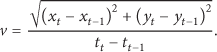
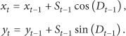
Predict_Trajectory: this function predicts the velocity of the trajectory. A simple approach is to use the two most recent target positions, that is,
Intersect_Trajectory: this function checks whether the trajectory intersects with the FOV and predicts the expected time of the intersection. This function is executed by all nodes which receive the “target trajectory” information from a neighboring node. Trajectory intersection with the FOV of a sensor node is computed by basic algebra. The expected time to intersect the node is estimated by

where
Goto_Sleep: this function shuts down the sensor node for single time period. It consumes the least amount of energy of all available actions.

Target prediction and intersection. Node j estimates the target trajectory and sends the trajectory information to its neighbors. Node i checks whether the predicted trajectory intersects with its FOV and computes the expected arrival time.
4.2. Set of States
We abstract the application by the following three states at every node.
Idle: this state indicates that there is currently no target detected within the node's FOV and the local clock is too far from the expected arrival time of any target already detected by some neighbor. If the time gap between the local clock
Awareness: there is currently also no detected target in the node's FOV in this state. However, the node has received some relevant trajectory information and the expected arrival time of at least one target is in less than
Tracking: this state indicates that there is currently at least one detected target within the node's FOV. Thus, the sensor node performs tracking frequently to achieve high tracking performance.
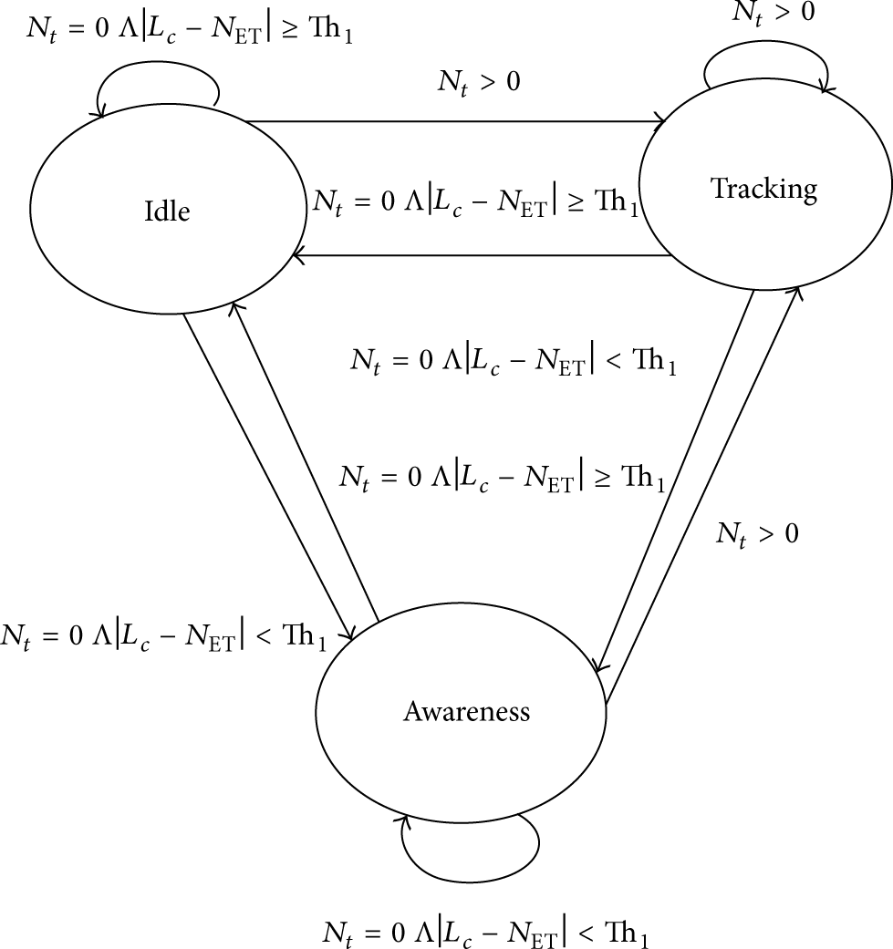
State transition diagram. States change according to the value of two application variables
Obviously, the frequency of executing Detect_Targets and Track_Targets depends on the overall objective, that is, whether to focus more on tracking performance or energy consumption. The states can be identified by two application variables, that is, the number of detected targets at the current time
Initially each node has no idea about which task to perform at which state. They learn this scheduling online over time. For example, Track_Targets is necessary task to keep tracking when the target is in FOV. The application learns online about the next task to execute based on our proposed methods. If the sensor node does not perform the Track_Targets task when the target is in FOV, there is a chance to miss the target which implies less tracking quality. But this situation could provide better energy efficiency, since Track_Targets task consumes the highest amount of energy among all the tasks. So, selection of a particular task at each time step or scheduling of tasks provides an impact on overall tracking quality/energy consumption tradeoff.
Figure 3 depicts the state transition diagram where
4.3. Reward Function
The reward function is a key system component for expressing the effect of the task execution on the system performance and resource consumption. Thus, both aspects should be covered by the reward function. Among the various options we simply merge energy consumption and system performance using a balancing parameter. In detail, the reward function in our algorithm is defined as
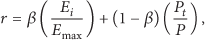
where the parameter β balances the conflicting objectives between
5. Online Learning Methods for Task Scheduling
We use RL, CRL, and Exp3 for the task scheduling in a multitarget tracking application. These three methods are online machine learning methods for task scheduling. RL and CRL are reinforcement learning methods. In RL, we do not exchange information among neighboring nodes. In CRL and Exp3, we exploit cooperation by exchanging trajectory information among neighboring nodes. In the following subsections we briefly describe the three learning methods and explain their key parameters. For our experiments we abstract the tracking application with the same tasks, states, and reward function.
5.1. Independent Reinforcement Learning (RL)
RL task scheduling follows the work of Shah and Kumar [14] which uses traditional Q learning [15] as online learning strategy. In Q learning the scheduling policy is represented by a two-dimensional matrix
The main idea of RL is to allow each individual sensor node to self-schedule its tasks and allocate its resources by learning their usefulness in any given state while honoring the application defined constraints and maximizing the total amount of reward over time.
In Q learning every agent needs to maintain a Q matrix for the value functions. Initially all entries of the Q matrix are zero and the agent of the nodes may be in any state. Based on the application defined variables, the system goes to a particular state. Then it performs an action which depends on the status of the nodes. It calculates the Q value for this (state, action) pair as

where
Algorithm 1 depicts the RL algorithm.
(1) Initialize (2) (3) Determine current state s by application variables (4) Select an action a which has the highest Q value (5) Execute the selected action (6) Calculate Q value for the executed action (7) Calculate the value function for the executed action (8) Shift to next state based on the executed action (9)
5.2. Cooperative Reinforcement Learning (CRL)
The CRL task scheduling follows a cooperative

for all s, a.
In (5),

In (6),
An important aspect of an RL-framework is the tradeoff between exploration and exploitation [20]. Exploration deals with randomly selecting actions which may not have higher utility in search of better rewarding actions, while exploitation aims at the learned utility to maximize the agent's reward.
In our proposed algorithm, we use a simple heuristic where exploration probability at any point of time is given by

where
The eligibility trace is updated by the following rule:


Algorithm 2 depicts the cooperative
(1) Initialize (2) (3) Determine current state s by application variables (4) Select an action a, using policy (5) Execute the selected action (6) Calculate reward for the executed action (3) (7) Update the learning rate (11) (8) Calculate the temporal difference error (6) (9) Update the eligibility traces (10) (10) Update the Q value (5) (11) Shift to next state based on the executed action (12)
The learning rate α is decreased slowly in such a way that it reflects the degree at which a state-action pair has been chosen in the recent past. It is calculated as

where ζ is a positive constant.
5.3. Bandit Solvers (Exp3)
We use the classical adversarial algorithm Exp3 (Exponential-weight algorithm for Exploration and Exploitation) for the task scheduling [18].
Algorithm 3 depicts the bandit solver algorithm Exp3.
(1) Parameters: Number of tasks A, Factor (2) Initialization: (3) (4) Determine current s based on application variables (5) Select an action (6) Execute the selected action (7) Calculate the reward: (8) Update the weights: (9) Calculate the updated probability distribution: (10) (11) Shift to next state based on the executed action (12)
In Exp3 the parameter κ controls the probability with which arms are explored in each round. At each time step t, Exp3 draws an action a according to the distribution
Exp3 works by maintaining a list of weights
6. Experimental Results and Evaluation
We evaluate the task scheduling methods using a WSN multitarget tracking scenario implemented in a C# simulation environment. The simulator consists of two stages: the deployment of the nodes and the execution of the tracking application. In our evaluation scenario the sensor nodes are uniformly distributed in a 2D rectangular area. A given number of sensor nodes are placed randomly on this area which can result in partially overlapping FOVs of the nodes. However, placement of nodes on the same position is avoided. Network parameters such as the number of nodes, the sensor radius, and the transmission radius can be configured in our simulator. Once these network parameters are configured, we can run the simulation with our selected algorithm.
Targets move around in the area based on a Gauss-Markov mobility model [22]. The Gauss-Markov mobility model was designed to adapt to different levels of randomness via tuning parameters. Initially, each mobile target is assigned a current speed and direction. At each time step t, the movement parameters of each target are updated based on the following rule:
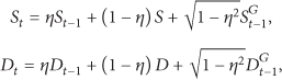
where
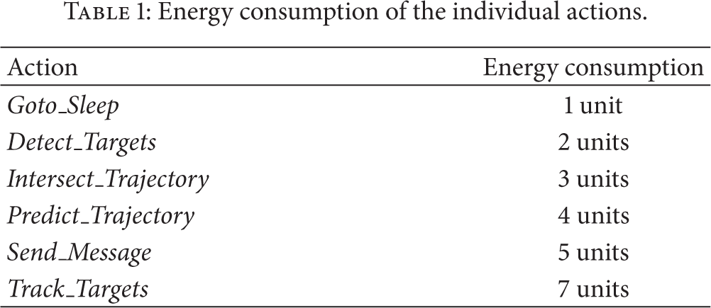
In our simulation we limit the number of concurrently available targets to seven. The total energy budget for each sensor node is considered as 1000 units. Table 1 shows the energy consumption for the execution of each action. We set the discount-factors
Energy consumption of the individual actions.
For our evaluation we perform the following four experiments with the following assumptions of parameters.
To find out the tradeoff between tracking quality and energy consumption, we set the balancing factor β of the reward function between
We vary the network size to check the tradeoff between tracking quality and energy consumption. We consider three different topologies consisting of 5, 10, and 20 sensor nodes where the coverage ratio is 0.0029, 0.0057, and 0.0113, respectively. The coverage ratio is defined as the ratio of the aggregated FOV of all deployed sensor nodes over the area of the entire surveillance area. We keep the balancing factor
We set the randomness of moving targets η to one of the following values
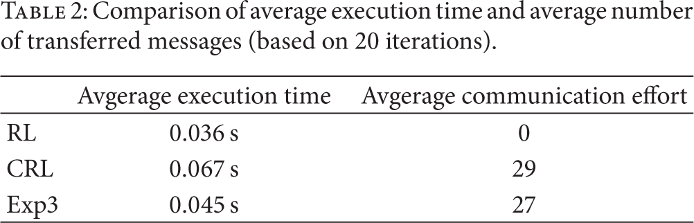
We evaluate RL, CRL, and Exp3 in terms of average execution time and average communication effort. These values are measured from twenty iterations and represent the mean execution times and the mean of Send_Message task executions.
Figure 4 shows the results of our first experiment. Each data point in these figures represents the average of normalized tracking quality and energy consumption of ten complete simulation runs. The results show the tracking quality/energy consumption tradeoff for RL, CRL, and Exp3 by varying the balancing factor β between
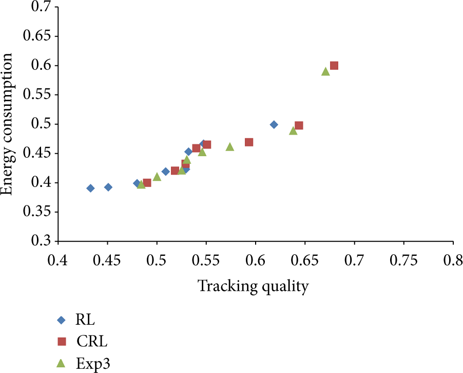
Tracking quality/energy consumption tradeoff for RL, CRL, and Exp3 by varying the balancing factor of the reward function β.
Figure 5 shows the results of our second experiment. In this experiment, each data point represents the average of normalized tracking quality and energy consumption of ten complete simulation runs by varying the network size to one of the values

Tracking quality/energy consumption tradeoff for RL, CRL, and Exp3 by varying the network size.
Figures 6, 7, and 8 show the results of our third experiment. In this experiment, each data point represents the average of normalized tracking quality and energy consumption of ten complete simulation runs by varying the randomness of moving objects η to one of these values

Tracking quality/energy consumption tradeoff for RL, CRL, and Exp3 by varying the randomness of target movement,

Tracking quality/energy consumption trade-off for RL, CRL and Exp3 by varying the randomness of target movement,

Tracking quality/energy consumption tradeoff for RL, CRL, and Exp3 by varying the randomness of target movement,
Table 2 shows the comparison of RL, CRL, and Exp3 in terms of average execution time and average communication effort. These values are derived from twenty iterations and represent the mean execution times and the mean of Send_message task executions. We find that RL is the most resource-aware scheduling algorithm. Exp3 requires 25% and CRL requires 86% more execution time, respectively. The communication overhead is similar for both Exp3 and CRL.
Comparison of average execution time and average number of transferred messages (based on 20 iterations).
7. Conclusion
In this paper we applied online learning algorithms for resource-aware task scheduling in WSNs. We analyzed and compared the performance of online task scheduling methods based on the three learning algorithms: RL, CRL, and Exp3. Our evaluation results show that these methods provide different properties concerning achieved performance and resource-awareness. The selection of a particular algorithm depends on the application requirements and the available resources of sensor nodes.
Future work includes the application of our resource-aware scheduling approach to different WSN applications, the implementation on our visual sensor network platforms [23], and the comparison of our approach with other variants of reinforcement learning methods.
Footnotes
Conflict of Interests
The authors declare that there is no conflict of interests regarding the publication of this paper.
Acknowledgments
This work was supported in part by the Erasmus Mundus Joint Doctorate in Interactive and Cognitive Environments, which is funded by the EACEA Agency of the European Commission under EMJD ICE FPA no. 2010-0012, and the EPiCS project funded by the European Union Seventh Framework Programme under Grant Agreement no. 257906.