Sage Journals: Discover world-class research

Abstract

Condition assessment (CA) of bearings can be performed by using left-right hidden Markov models, because of the monotonically increasing pattern of the bearings degradation. Classical CA approaches assume that all possible system states are fixed and known a priori. The training of the system is performed offline at once with data from all of the system states. These assumptions significantly impede condition assessment applications in case that all the possible states of the system are not known in advance, or changes in environmental or operative conditions occur during the tool's usage. To overcome these limitations, we propose combining left-right continuous HMMs (CHMM) with a change point detection algorithm for (i) estimating, from historical observations, the initial number of the CHMM states and the initial guess of its model parameters and (ii) updating the state space as well as the model parameters during monitoring. Moreover, to deal with multidimensional sensor measurements, we propose using kernel principal component analysis for dimensionality reduction. Qualitative and quantitative evaluations of the proposed methodology have been performed using both simulated and real data from the NASA benchmark repository. Compared to state of the art techniques, the proposed methodology results in (i) an improvement of the HMM training phase in terms of iterations number; (ii) the detection of unknown states at an early stage; and (iii) an effective change of the CHMM's structure to represent the degradation processes more accurately in presence of unknown conditions.

1. Introduction

Machines and equipments breakdown in industrial environments can have significant impact in the profitability of a business. Maintaining the engineering assets in operating conditions is an industrial and economical requirement. Nowadays optimization strategies for maintenance are an important part of research for companies [1, 2], since, next to energy costs, maintenance spending due to equipment or machine failure can be the largest part of the operational budget [3].

Corrective maintenance [1, 4], which is the system maintenance strategy subject of this work, is based on condition monitoring and is performed after a degradation modality emerges in a system, with the goal of preventing the system from failing. A fundamental requirement of this strategy is the detection of the abnormal behavior, that will lead to the system failure, at an early stage in order to give enough time to perform the repair operations.

Industrial equipments and their components are often characterized by a very complex structure. For this reason the usage of mathematical models for condition monitoring can represent an arduous task. On the other hand, industrial machines are usually equipped with monitoring devices (sensors placed in critical parts of the system under study) which are able to record and collect large amount of measurements. Given the availability of these huge amounts of data, the methodology proposed in this paper will focus on data-driven models [5], which are based on machine learning approaches.

The classical usage of data-driven techniques consists of two phases: a first training phase in which a preprocessing of the historical raw sensory data is performed in order to extract relevant features, which will be then exploited to learn the parameters of behavioral models of the considered machine and a second application phase, during the runtime of the system, in which the trained model is used along with runtime measurement to evaluate the health condition of the machine. The advantage of such approaches is that, for a well monitored system, there is no need for knowledge of the system's internal physical mechanism or for a prior mathematical model to represent the system degradation.

Several data-driven models for condition monitoring have been proposed, such as clustering techniques [6], data-mining approaches [7], support vector machines [8], dynamic Bayesian networks [9], and hidden Markov models [10, 11]. Hidden Markov models (HMMs) have been shown to be effective pattern recognition tools in a large variety of recognition tasks. They have been successfully applied to condition monitoring of manufacturing machines [12, 13] as well as in other application domains ranging from speech recognition [14] to intrusion detection in computer systems [15].

The common usage of hidden Markov hodels, especially for condition assessment applications, consists of dividing the degradation pattern of the historical data of the system under study into different degradation levels, from normal to deeper degradation (i.e., good, partially worn, seriously worn, broken), and training either several HMMs, each one corresponding to observations (features) from a particular degradation level [16 –19] or training a single HMM using historical observations corresponding to the normal behavior of the system [19 –23]. Online condition assessment is then performed by selecting the HMM that, on new incoming data, gives the highest likelihood or by detecting an abnormality if the likelihood is lower than a threshold defined for the normal behavior [19]. However, the latter approach is not well suited to condition assessment of industrial systems, as it can be used only for anomaly detection. Indeed, such approach is only able to detect a condition that is different from the considered normal behavior in the training phase.

Another approach [14] consists of training a single HMM by using the sensor measurements corresponding to the entire lifetime of the system, by setting the number of states equal to the number of degradation stages contained in the training history. By using this approach, the model maps each degradation phase to a state of the HMM. The condition assessment is performed online on new incoming data by calculating the Viterbi path [24] which returns the most probable state sequence.

The approaches described above assume that all possible system condition states are known a priori and that training data sets from the associated states are available. In addition, the training procedure has to be performed offline and only once at the beginning, with the available training set. For this reason, the trained models are able to recognize only the conditions contained in the training data. These assumptions significantly impede component diagnosis applications when:

it is difficult to identify and train all of the possible states of the system in advance;

environmental factors or operative conditions change during the tool's usage.

Since industrial machines are constantly subjected to updates, changes of configurations or changes of working conditions, a need for models that are able to automatically adapt to new situations, by dynamically learning the structure and the parameters, is required. To the best of our knowledge, such approach has only been used by Lee et al. [25], whom proposed a modified hidden Markov model with variable state space to estimate the current state of system degradation as well as to detect unknown faults at an early stage. A multivariate statistical process control is used to detect the occurrence of an unknown condition by measuring the deviation of the current signal from a reference signal representing prior known states; then the HMM is updated by including a new state. The limitation of this approach is that (i) one should collect reference signal representing prior known states and (ii) define a parametric model (Gaussian in the case of [25]) of the observation signals.

To overcome the abovementioned drawbacks of most of the state of the art HMM-based condition assessment approaches, we proposed in [26] a methodology based on HMMs which is able to perform (i) an automatic estimation of the initial parameters and number of states of the model and (ii) an online adaptation of the model structure, together with the online learning of the parameters, in presence of not stable conditions. The proposed approach aims to diagnose the degradation processes of industrial systems using a variable state space left-right continuous HMM (CHMM), by integrating a change point detection (CPD) algorithm [27].

The CPD algorithm allows detecting the dynamic changes of machine condition and hence of the HMM parameters, by discovering time points at which the properties of the input time-series data change, corresponding to the (signal) segmentation of the observed data stream. The detected segments correspond to the different states of the machine. In this work, as a further contribution, we evaluate the reliability of the data driven identification of the number of (possible) system's states by means of clustering techniques and the Dunn's validity indexes [28].

Concerning the online condition assessment, the comparison between the estimated most-likely state, by the Viterbi algorithm [24], and the CPD detected segments (states) allows fast failures detection. Moreover, since the CPD algorithm is independent from the density model of the observation, in comparison with the method of Lee et al. [25], our proposal is more effective as it is independent of prior data and allows faster detection of unknown conditions.

The used CPD algorithm is able to handle 1-dimensional time series, while industrial machines are usually equipped with several sensors for which multiple features can be extracted, resulting in a multidimensional observation vector. To have an accurate modeling for real world cases, it is essential to consider as much information as possible related to system changes, carried by multiple signals. In this work we propose applying kernel principal component analysis (KPCA) [29 –31] for dimensionality reduction. KPCA, being able to effectively deal with nonlinear data, embeds the information coming from all the measurements in to a 1-dimensional time series and allows a faster detection of condition changes by the CPD algorithm.

Although it is adaptable to a wide range of health estimation problems, we applied the proposed methodology on bearings condition monitoring. This choice derives from the fact that, being the most common mechanical elements in industry, bearings are the components which most frequently fail in rotating machines [32]. Furthermore, given the nature of the component, we can assume that the degradation pattern of bearings is monotonically increasing and, therefore, the use of left-right HMMs is well-motivated.

The rest of the paper is organized as follows. Section 2 gives a short overview of the used concepts and methods, namely, continuous left-right hidden Markov models, the preprocessing and features extraction techniques, and the change point detection algorithm. In Section 3, we provide a detailed description of the proposed approach. In Section 4 experimental results are discussed. The conclusion and future research directions are given in Section 5.

2. Methods and Algorithms

Before going into a more detailed discussion of the proposed approach, an overview of the techniques used in this paper is given in this section.

2.1. Left-Right Continuous Hidden Markov Models

Left-right vontinuous hidden Markov models (CHMMs) [14] are dynamic models in which there are two types of variables: a state variable describing the system state, which is never observed/measured directly (hidden), and an observation variable which is related to the hidden state.

A left-right CHMM λ = (A, C, μ, U, π) is characterized by the following:

N, the number of states in the model, S = {S₁, …, S_N} the set of states, and s_t the state at time t,

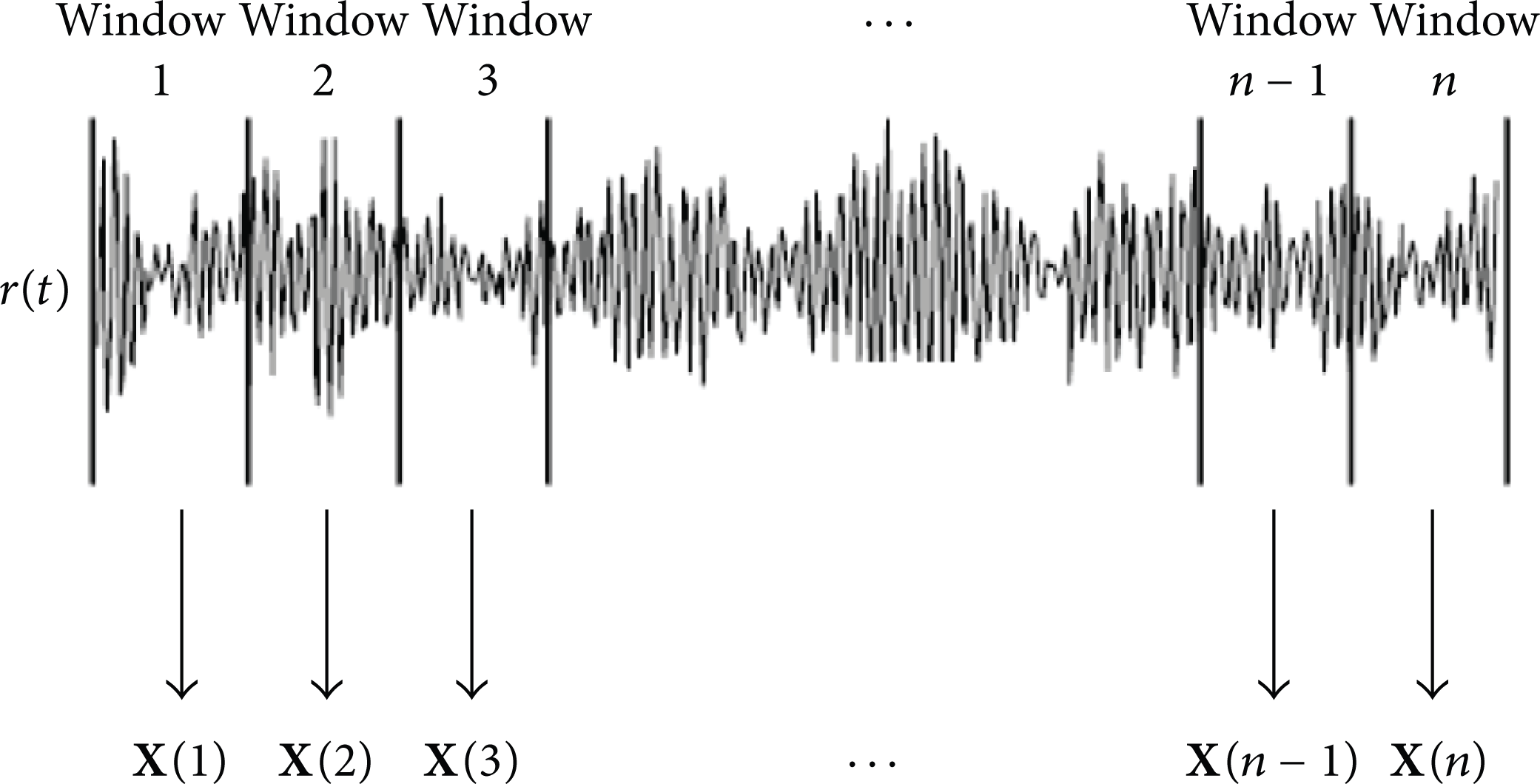
the state transition probability distribution A = {a_ij} where

a_{i j} = P (s_{t + 1} = S_{j} ∣ s_{t} = S_{i}), 1 \leq i, j \leq N,

(1)

X_t, the continuous observation vector emitted from the state at time t,

the observation density, represented by a finite mixture:

b_{j} (X) = \sum_{m = 1}^{M} ‍ c_{j m} ℵ (X, μ_{j m}, U_{j m}), 1 \leq j \leq N,

(2)

where X is the vector being modeled, c_jm the mixture coefficient for the mth mixture in state j, and ℵ is any log-concave or elliptically symmetric density (usually a Gaussian), with mean vector μ_jm and covariance matrix U_jm for the mth mixture component in state j. The parameters c_jm, μ_jm, and U_jm, are the coefficients of C, μ and U, respectively,

the initial state distribution π = {π_i} where

π_{i} = P (s_{1} = S_{i}), 1 \leq i \leq N .

(3)

It is proved that the probability density function of (2) can be used to approximate, arbitrarily closely, any finite, continuous density function [33]. Hence it can be applied to a wide range of problems.

The left-right topology has the property that the state index can either increase or stay the same, as time goes on. In this case, the following holds for the coefficients of the transition matrix:

a_{i j} = 0, j < i,

(4)

a_{i j} = 0, j > i + Δ,

(5)

a_{N N} = 1,

(6)

a_{N i} = 0, i < N,

(7)

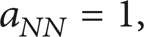
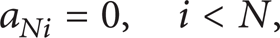
where (4) avoids transition to previous states and (5) avoids jumps of more than Δ states, while the state N is an absorbing state. Moreover, since the model starts from state S₁, the initial state probabilities have the following property:

π_{i} = \{\begin{cases} 0 & i \neq 1 \\ 1 & i = 1 . \end{cases}

(8)

For CHMMs applied to condition monitoring, learning and inference procedures can be used.

Learning: adjust the model parameters λ = (A, C, μ, U, π) in order to maximize the probability P(X∣λ); that is, for the considered CHMM structure, find the model parameters that better fit the historical sensor measurements X. This problem is solved through the Baum-Welch algorithm [34].

Decoding: given a model λ = (A, C, μ, U, π) and a sequence of sensor measurements X = X₁, X₂, …, X_T, find the hidden state sequence S = s₁, s₂, …, s_T that has most likely produced the observation sequence. The solution of this problem is given by the Viterbi algorithm [24].

In the next section we will describe how we can fit the multidimensional time-series input coming from the machine sensors into a CHMM model.

2.2. Feature Extraction and Dimensionality Reduction

In this paper, the inputs are vibration signals originating from sensors on the machine under study. For this purpose, one accelerometer or more accelerometers are placed in the component housing and are used to translate the vibrations emitted to an electric continuous signal. For each sensor, the electric signal measured is then sampled at a predefined sampling frequency. The monitoring system of the machine acquires and stores such samples one at a time, under the form of a digital signal, which represents the raw input data, referred to as r(t) with 1 ≤ t ≤ T. It is assumed that a characteristic shape of the measured vibration is related to the actual condition of the component.

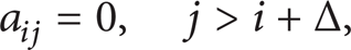
Due to the high sampling frequency that is often used, a high-dimensional signal is measured. Moreover, consecutive values of a time series are usually not independent but highly correlated; thus there is a lot of redundancy. Hence, rather than looking at each point in time sequentially to detect anomalies, it is common to use sliding windows of length L. Within each window, k and d features are calculated, resulting in a vector of d components X(k) = [x₁(k), x₂(k), …, x_d(k)]^T. Finally, the raw signal r(t) is transformed in a multivariate time series as (10). The process is illustrated in Figure 1. Consider

Raw signal: r (t) = r (1), \dots, r (T) ↓ features extraction,

(9)

\begin{matrix} X (t) = [X (1), \dots, X (n)], \\ X (t) = [[\begin{bmatrix} x_{1} (1) \\ ⋮ \\ x_{d} (1) \end{bmatrix}], \dots, [\begin{bmatrix} x_{1} (n) \\ ⋮ \\ x_{d} (n .) \end{bmatrix}]] \end{matrix}

(10)

Figure 1:

Feature extraction from raw signals.

In this work, as also explained in Sections 4.2.1 and 4.2.3, we considered windows of size L = 20480 (fixed by the used data set) and d = 3 time domain features, namely, the mean, the root mean square, and the kurtosis, of the sensory signals. It has to be noted that frequency [35] (i.e., Fourier transform) or time-frequency [36, 37] (i.e., wavelet transform) domain features could be used as well.

Since the considered CPD algorithm is able to process 1-dimensional signals, a further dimensionality reduction technique has to be applied on the d-dimensional features vectors. In this paper, kernel principal component analysis (KPCA) [29 –31] is applied as a technique for dimensionality reduction.

In the literature, principal component analysis (PCA) has been extensively used as a features extraction technique for condition assessment applications [18]. However, KPCA has been shown to perform better than the standard PCA for processes with particularly nonlinear characteristics [31]. The basic idea of KPCA is that when the variations are nonlinear, the data can always be mapped into a higher-dimensional space, by means of nonlinear kernel functions, in which they vary linearly. In this work Gaussian radial basis kernels have been used. The reader is referred to [29, 31] for the details on KPCA.

The main advantages of KPCA are the fact that (i) it does not involve nonlinear optimization [29] since it requires only linear algebra, making it as simple as standard PCA which requires only the solution of an eigenvalue problem; (ii) due to its ability to use different kernels, it can handle a wide range of nonlinearities; (iii) it does not require the number of components to be extracted be specified prior to modeling.

Applying KPCA on feature vectors X(t) generates a 1-dimensional time-series, y(t), (t = 1, …, n), which can be used as input to the CPD algorithm.

2.3. Change Point Detection Algorithm

The change point detection approaches apply data mining techniques to identify the time points at which the changes, that is, events, occur. This has been discussed in several applications such as fraud detection [38], rare event discovery [39], event/trend change detection [27], and activity monitoring [40].

In [27] a method has been proposed for the detection of the appropriate set of number of points that minimizes the error in fitting a predefined function using maximum likelihood. There is no fixed number of change-points to be detected. Moreover, no constraints are imposed on the class of functions that will be fitted to the subsequences between successive change-points.

Following the notation in [27], let y(t), (t = 1, …, n), be the time series to be segmented. It is assumed that the time series can be modeled mathematically, where each model is characterized by a set of parameters. The problem of change-points detection is formulated as finding a piecewise segmented model, given by the following:

\begin{matrix} Y = f_{1} (t, v_{1}) + e_{1} (t), (1 < t \leq θ_{1}), \\ = f_{2} (t, v_{2}) + e_{2} (t), (θ_{1} < t \leq θ_{2}), \\ = \dots \\ = f_{l} (t, v_{l}) + e_{l} (t), (θ_{l - 1} < t \leq n), \end{matrix}

(11)

where f_i(t, v_i) is the function (with its vector of parameters v_i) that is fitted to the segment i. The θ_i's are the change-points between successive segments, and e_i(t)'s are error terms.

Several types of basis functions, f_i(t, v_i), can be considered, for example, algebraic polynomials, wavelet, Fourier, and so forth [41]. In our current implementation polynomial fitting functions have been selected, since they represent a good compromise between expressiveness power and computational effort.

In [27], two CPD approaches have been proposed, the batch (offline) and the incremental (online). In the batch version, the entire data set is available in advance, from which the best set of change-points is determined. In the incremental version, the algorithm receives new data points one at a time and determines if the new observation causes a new change-point to be discovered. Both approaches are summarized here after. Details on the implementation can be found in [27].

2.3.1. Batch Algorithm

The batch CPD algorithm assumes that the entire time series data is available before the analysis begins. Let S be the residual sum of squares for the selected fitting function that maintains time points t_i, t_{i + 1}, …, t_j. In this paper we define the likelihood criterion as $L (i, j) = S$ since we used a homoscedastic error model [27].

The key idea behind the algorithm in [27] is that, at every iteration, each segment is examined to see whether it can be split into two significantly different segments. The splitting procedure can be illustrated by a consideration of the first stage, since all subsequent stages consist of equivalent scaled-down problems.

Let the data set cover the time points t₁, t₂, …, t_n. The change-point in the first stage is the j minimizing $L (1, j) + L (j + 1, n)$ , say j^*. Here j^* is defined as follows:

L (1, j^{*}) + L (j^{*} + 1, n) = \min_{p \leq j \leq n - p} L (1, j) + L (j + 1, n) .

(12)

The range of j depends on the fact that at least p points are needed for model fitting in each segment.

At the second stage, the best candidate change-points c₁ and c₂ of each of the two segments are located. The selection of the better of these two candidates yields a division of the original sequence into three segments. Assuming that point c₁ is chosen, now the likelihood criteria of the model becomes as follows:

L = (L (1, c_{1}) + L (c_{1} + 1, j^{*}) + L (j^{*} + 1, n)) < (L (1, j^{*}) + L (j^{*} + 1, c_{2}) + L (c_{2} + 1, n)) .

(13)

The procedure above is repeated until a stopping criterion is reached. Once the algorithm has detected all “real” change-points, adding any more change-points the likelihood will increase. Therefore, the algorithm should stop when the likelihood criteria becomes stable or starts to increase. Formally, if in iterations z and z + 1 the respective likelihood criteria values are $L_{z}$ and $L_{z + 1}$ , the algorithm should stop if

\frac{(L_{z} - L_{z + 1})}{L_{z}} < s,

(14)

where s is a user-defined stability threshold. When stability threshold s is set to 0%, the algorithm stops only when the likelihood criteria starts increasing.

2.3.2. Incremental Algorithm

In an online setting, the change-point detection must proceed concurrently with data collection. The key idea of the incremental algorithm is that if the next data point collected by the sensor reflects a significant change in phenomenon, then the likelihood of being a change-point is going to be smaller than the likelihood that it is not. However, if the difference in likelihoods is small, we cannot definitively conclude that a change did occur, since it may be the artifact of a large amount of noise in the data. Therefore a user-defined likelihood increase threshold is introduced. Consider

\frac{(L_{no_change} - L_{change})}{L_{no_change}} > δ,

(15)

where δ is a user-defined likelihood increase threshold.

Suppose that the last change-point was detected at time t_{l − 1}. At time t_l the algorithm starts by collecting enough data to fit the regression model. Suppose at time t_j a new data point is collected. The candidate change-point is found by determining t_i, with likelihood criterion $L_{\min} (l, j)$ , such that

L_{\min} (l, j) = \min_{l < i \leq j} L (l, i) + L (i + 1, j) .

(16)

If this minimum is significantly smaller than $L (l, j)$ , that is, the likelihood criteria of no change-points from t_l to t_j, then t_i is a change-point. Otherwise, the process should continue with the next point, that is, t_{j + 1}.

In the incremental algorithm, execution time is a significant factor. If enough information is stored, some of the calculations can be avoided. Thus, at time t_{j + 1} to find likelihood criteria

L_{\min} (l, j + 1) = \min_{l < i \leq j} L (l, i) + L (i + 1, j + 1),

(17)

it is only necessary to calculate $L (i + 1, j + 1)$ , since (l, i) was calculated in the previous iteration.

It should be noted that if a change-point is not detected for a long time, the successive computations become increasingly expensive. A possible solution is to consider a sliding window of only the last q points.

3. Framework

The framework of the proposed approach is illustrated in Figure 2. As discussed in the introduction, the methodology is applied in two phases, the training (phase 1) and the online application (phase 2).

Figure 2:

Framework of the proposed approach.

3.1. Phase 1: Estimation of the Initial Number of States and Parameters Initialization

During the first phase, we assume that enough historical raw data have been collected from the monitoring system of the machine under study. Such data can be measurements from multiple sensor types (temperature, pressure, acceleration,…etc.). For each sensor measurement, as described in Section 2.2, we apply the feature extraction, yielding multidimensional feature vectors X(t), on which we apply KPCA dimensionality reduction. The resulting 1-dimensional signal, y(t), is then input to the CPD algorithm, which in turn delivers (detects) N^* segments.

Each segment is mapped to a HMM state. The intuition of this approach comes from the assumption that there is a correlation between observations and states. Thus, a variation in the condition of the system corresponds to a change in the behavior of the sensorial measurements.

Once the number of states (N^*) has been estimated, and knowing the end-points of each segment, the initialization of the HMM parameters λ₀ = (π₀, A₀, C₀, μ₀, U₀) can be performed. Since left-right HMMs are considered, π₀ is initialized by using (8). Using (4), (6), (7), and (5) with Δ = 1, the transition matrix A₀ is initialized as follows:

a_{i j} = \frac{# tr (i, j)}{# s_{i}}, j = i + 1

(18)

\forall i, a_{i i} = 1 - \sum_{j \neq i} ‍ a_{i j},

(19)

where # tr ⁡ (i, j) is the number of transitions from segment i to j (which is equal to 1 if left-right HMMs) and # s_i the number of data points in segment i. The transition matrix is ensured to satisfy the stochastic constraint, being ∀i, ∑^{j = 1}_Na_ij‍ = 1.

Concerning the coefficients μ_jm, U_jm, and c_jm relative to the observation density parameters (see equation (2)), they are estimated from the multidimensional features signal X(t) for each segment (state) 1 ≤ j ≤ N^* with the following equations:

\forall m, μ_{j m} = \bar{X (t)}, t \in j;

(20)

\forall m, U_{j m} = Cov (X (t)), t \in j,

(21)

where $\bar{X (t)}$ and Cov(X(t)) are, respectively, the mean vector and the covariance matrix of the multidimensional features signal. The mixture coefficients c_jm are initialized by using the uniform distribution, for each j and m: c_jm = 1/M, M being the number of mixtures.

Together with the features extracted from the training histories, the estimated initial parameters λ₀ are used as inputs to the Baum-Welch procedure. The obtained optimal model parameters, λ^*, of the N^*-states left-right CHMM, are then used in the following phase 2 for the online adaptive condition assessment.

3.2. Phase 2: Online Adaptive Condition Assessment

The application phase is performed on new incoming data which are referred to as testing signal in Figure 2. These raw data are acquired online, during the normal runtime of the machine under study and are collected one sample a time. When a window of predefined length L of points are acquired, the feature extraction procedure is executed to produce multidimensional features. Two parallel process are then executed: the trained CHMM is used to estimate the current system's state, while the online CPD algorithm keeps track of the encountered changes of conditions to possibly detect previously unknown situations. In particular:

for condition assessment, the multidimensional features signal is input to the inference algorithm, using the current N^*-states left-right CHMM model and its optimal parameters λ^*, to calculate, via the Viterbi algorithm [14], the most probable state sequence, given the observations up to that moment. The last state in the inferred sequence is then selected as the actual condition of the machine;

for possible HMM state and parameters update, we map the multidimensional features to 1-dimensional signal using the out-of-sample extension according to the kernel PCA parameters calculated in the training phase. The obtained 1-dimensional signal is input to the online CPD algorithm to detect possible changes, which could correspond to state changes. Here, we assume that an unknown situation is experienced by the system when the detected segments (change-points) exceed N^*, being the number of states of the optimal CHMM of the previous phase or iteration. In such case, when enough samples coming from the new condition are acquired, a new state is added to the CHMM, to obtain a new model with N^* = N^* + 1 states. The model parameters, λ^*, are also adapted to the new situation, by performing the training procedure as described above in phase 1, using the current testing signal together with the training histories.

4. Experimental Results

To verify the effectiveness of the proposed methodology, several experiments have been performed both on simulated and on real data. The simulated data were generated according to the parameters described in the example reported in [25], while condition monitoring data related to bearings taken from the NASA benchmark repository [42] have been used as real data. All the parameters concerning kernel PCA and CPD algorithms have been carefully estimated through linear searches.

4.1. Simulated Experiment

In this section we illustrate the performances of the proposed approach by means of a numerical example proposed in [25]. The goal of these experiments is to study the case in which some of the hidden states of the CHMM are not known in advance, but they appear during the normal functioning of the system.

To better illustrate the effectiveness of the proposed methodology we compare it to method of Lee et al. [25], denoted here after as modified HMM approach. Moreover, we evaluate the results according to two criteria:

the classification accuracy, defined as the percentage of states correctly classified by the Viterbi algorithm with respect to the true known state sequence,

the detection time, defined as the moment in time in which the unknown state is detected.

4.1.1. Data Generation

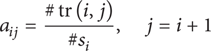
A training set composed of 5 histories from a 4-state CHMM has been generated. Supposing that two signals (X₁ and X₂) are monitored, the observation density follows a two-jointly Gaussian distribution. The CHMM parameters used to generate the training data are as follows:

\begin{matrix} π = [\begin{bmatrix} 1 \\ 0 \\ 0 \\ 0 \end{bmatrix}], A = [\begin{bmatrix} 0.99 & 0.01 & 0 & 0 \\ 0 & 0.99 & 0.01 & 0 \\ 0 & 0 & 0.99 & 0.01 \\ 0 & 0 & 0 & 1 \end{bmatrix}], \\ μ_{1} = [\begin{bmatrix} 20 \\ 20 \end{bmatrix}], μ_{2} = [\begin{bmatrix} 20 \\ 35 \end{bmatrix}], \\ μ_{3} = [\begin{bmatrix} 35 \\ 35 \end{bmatrix}], μ_{4} = [\begin{bmatrix} 35 \\ 20 \end{bmatrix}], \\ U_{1} = [\begin{bmatrix} 20 & 0 \\ 0 & 20 \end{bmatrix}], U_{2} = [\begin{bmatrix} 15 & 0 \\ 0 & 15 \end{bmatrix}], \\ U_{3} = [\begin{bmatrix} 15 & - 2 \\ - 2 & 15 \end{bmatrix}], U_{4} = [\begin{bmatrix} 5 & 0 \\ 0 & 5 \end{bmatrix}] . \end{matrix}

(22)

For each history, 500 data points have been sampled. One possible example of observable signals is illustrated in Figure 3.

Figure 3:

Scatter plot of the first simulated case. For the artificial experiment, 500 observation samples from a 4-state CHMM with 2 monitored signals (X₁ and X₂, following a 2-joint Gaussian observation distribution) have been sampled for 5 histories.

To evaluate the behavior of the proposed methodology under the presence of an unknown situation, we sampled the testing case using a CHMM with 5 states: for the first 4 states we used the same parameters as the training set, while a fifth (previously unknown) state has been added, with the following parameters:

μ_{5} = [\begin{bmatrix} 50 \\ 50 \end{bmatrix}], U_{5} = [\begin{bmatrix} 10 & 3 \\ 3 & 10 \end{bmatrix}] .

(23)

By knowing beforehand the true states sequence of the testing case as well as the the switch time to the fifth state (time 511), in the following we compare the classification accuracy and the unknown state detection time obtained by our method and by the modified HMM of Lee et al. [25].

4.1.2. Proposed Approach

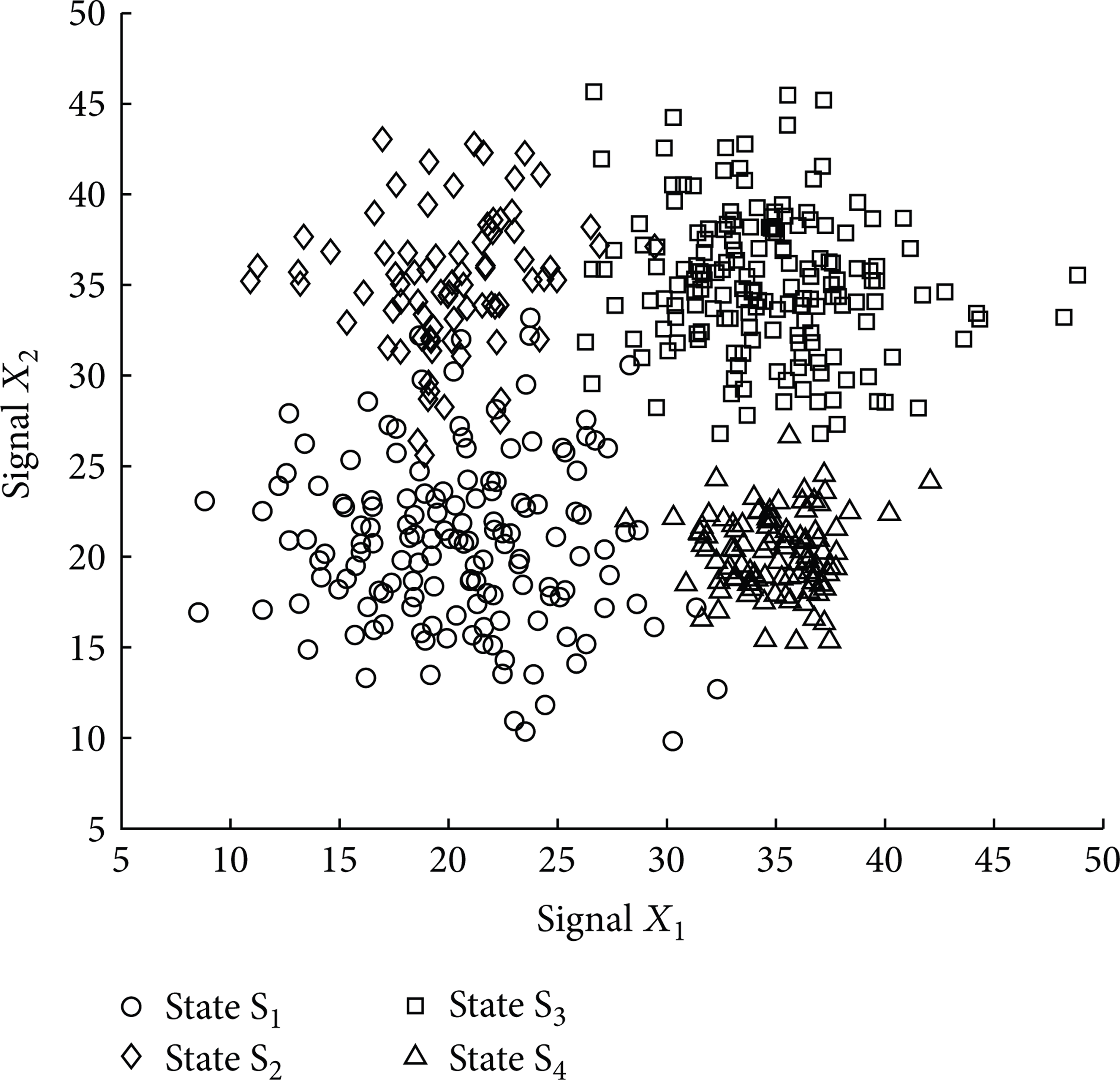
For each training history, we applied kernel PCA, using a Gaussian kernel with variance which is equal to 1, in order to reduce the 2-dimensional observation to a 1-dimensional signal. An example of dimensionality reduction is illustrated in Figure 4 for the first training history.

Figure 4:

Dimensionality reduction with KPCA. The information available in the two-dimensional signal shown in plots (a) and (b) is combined in a single signal shown in plot (c) using KPCA. This transformation keeps information related to changes in the original signals.

The obtained 1-dimensional signals have been input to the batch CPD algorithm to perform the initial states numbers estimation. As shown in Figure 5, the 4 segments are correctly detected. The selected parameters of the batch CPD algorithm are as follows: a second degree polynomial fitting function and a stability threshold s = 0.01 (see equation (14)).

Figure 5:

Initial states number estimation with batch CPD. The 4 segments associated with the 4 CHMM states are correctly detected.

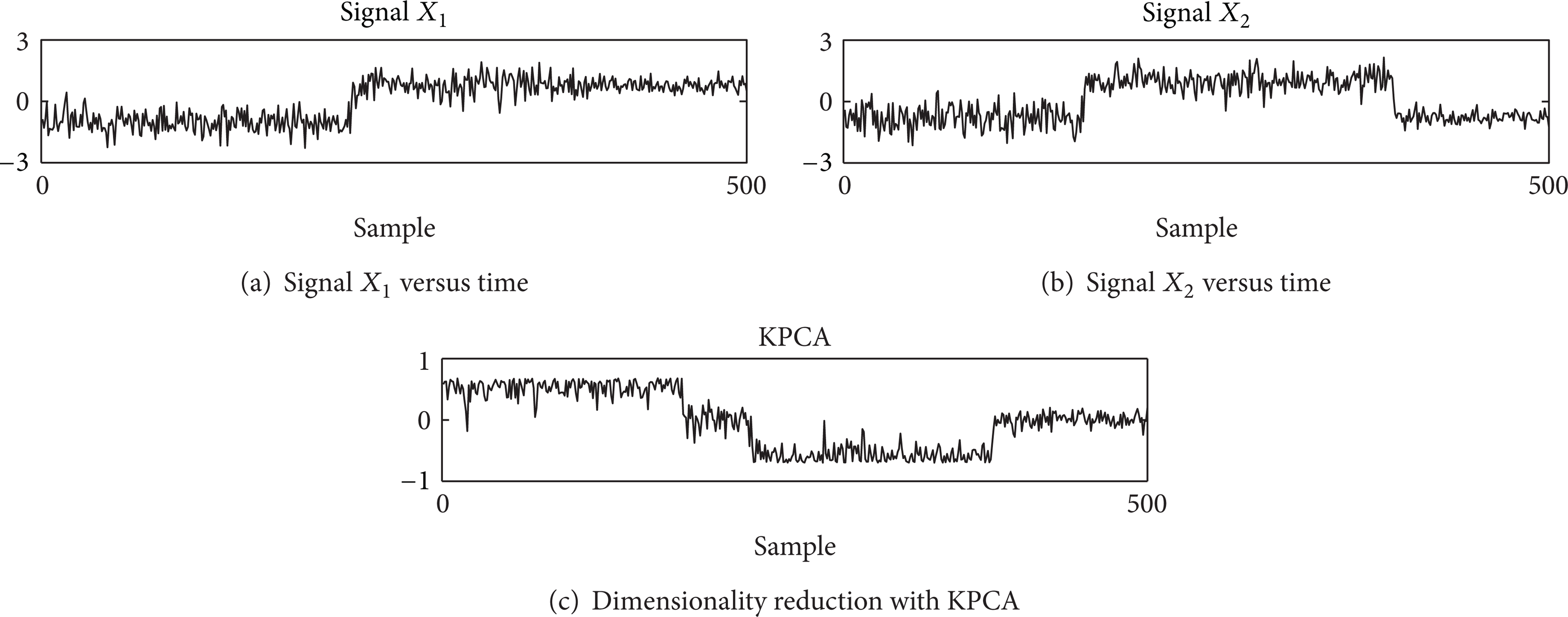
Once the initial number of segments is obtained, we consider a N^* = 4-state left-right CHMM model for which the parameter λ has to be estimated using the Baum-Welch algorithm. To evaluate the efficiency of the proposed initial parameters estimation approach, we performed 11 runs of the Baum-Welch algorithm using as initial values the estimated λ₀ as described in Section 3.1 and 10 randomly set λ₀'s. For these experiments, we selected a single Gaussian as observation density of the CHMM and a maximum number of 15 iterations.

Figure 6 shows that the learning procedure converges in 4 iterations when the initial parameters are set using the proposed approach, compared to the randomly set parameters. Moreover, the final likelihood value is comparable with the best random initialization.

Figure 6:

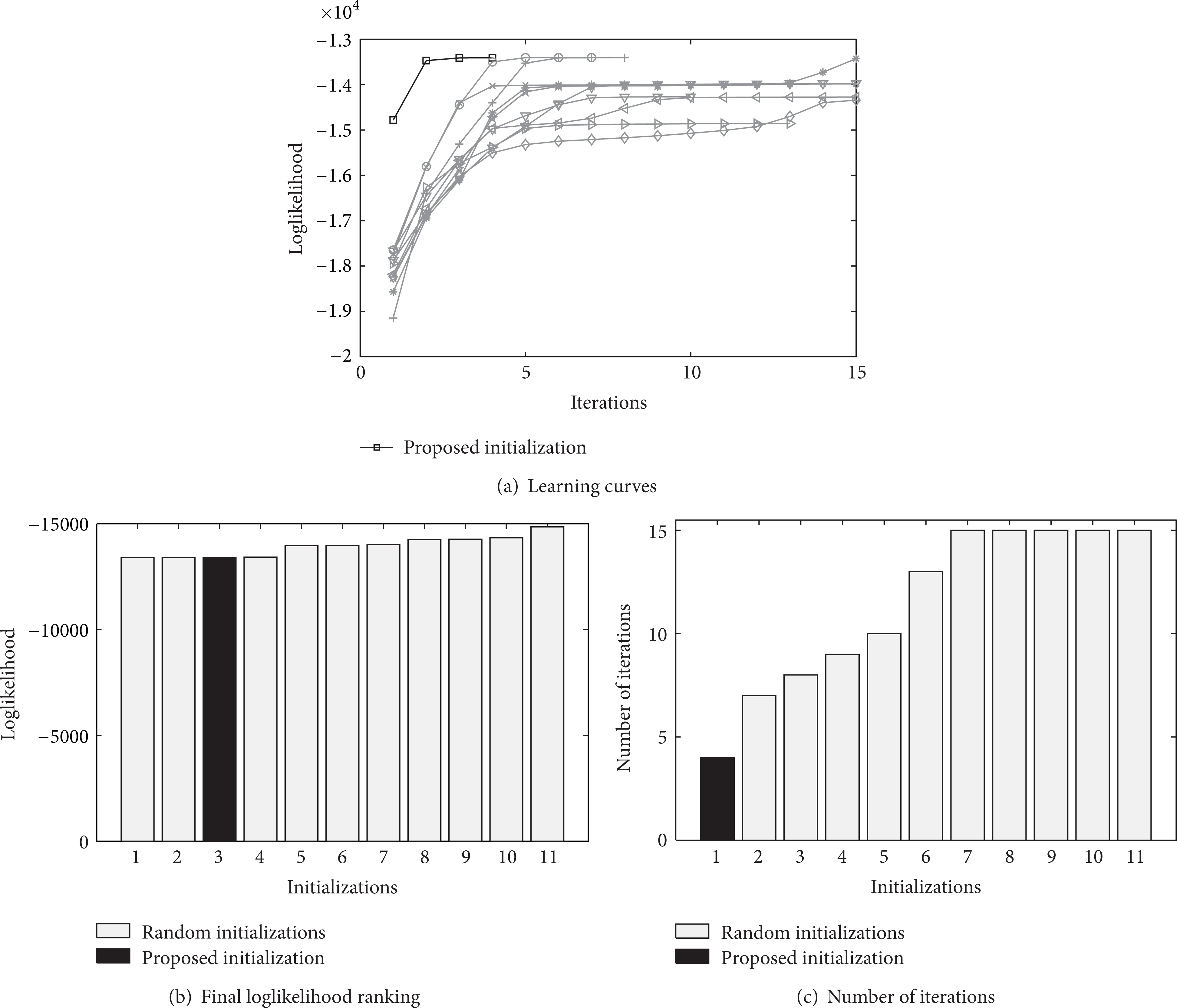
Training Evaluation, the proposed λ₀ estimation versus 10 randomly set λ₀. By using the proposed approach for parameters initialization the Baum-Welch algorithm converges after only 4 iterations (the fastest in this comparison) and the final likelihood value is comparable with the best random initialization.

The 4-state CHMM trained model is then used to perform the online condition assessment as described in Section 3.2. For these experiments we employed the following parameters for the online CPD algorithm: a first order polynomial fitting function and a likelihood threshold δ = 0.4 (see equation (15)).

As illustrated in Figure 7(d), until time 522, the trained 4-state CHMM has been used, and the Viterbi path correctly assesses the four states. At time 512 (denoted by the last cross in Figure 7(c)), the online CPD detects a further state. After 10 more data have been acquired, the CHMM is enriched with a new state, and the training procedure is executed again to estimate the paramters of a 5-state CHMM. From the time point 522 on, the new 5-state CHMM is used, for which the Viterbi path correctly assesses the fifth state until the end of the experiment. The accuracy achieved by the Viterbi path is 97.23% of correctly classified states in the sequence.

Figure 7:

Online condition assessment using the online CPD algorithm on the testing case. At time 512 the online CPD algorithm detects a further state, which is added to the original 4-state CHMM. From time 522 on, the fifth state, which was unknown during the training phase, is correctly assessed by the Viterbi algorithm.

4.1.3. Modified HMM Approach [25]

The results above have been compared to the ones using the approach of Lee et al. [25] that, in contrast to the proposed methodology which employs data mining and curve fitting techniques, is based on multivariate statistical tests.

The detection of a new state is performed by evaluating a statistically significant shift in the mean of the observation signal using the hotelling multivariate control chart (referred to as hotelling MCC as follows). Hotelling MCC considers as measure of similarity the Mahalanobis distance, denoted as $D^{2} (\bar{O}, μ_{i})$ , between the empirical mean $\bar{O}$ of the last b observations (set to 10 in our experiments) and the μ_i parameter relative to the state i, which is the most probable state given by the Viterbi path:

D^{2} (\bar{O}, μ_{i}) = b {(\bar{O} - μ_{i})}^{T} U_{i}^{- 1} (\bar{O} - μ_{i}),

(24)

where U_i is the covariance matrix relative to the most probable state i. If this statistic exceeds a certain threshold, called upper control limit (UCL), for more than R consecutive times, then a significant change is assumed in the process and a new state is added. R can be seen as a measure of the detection sensitivity of the algorithm, if R is increased, the detection algorithm may become more robust against false detections caused by the process randomness itself; on the other hand, the algorithm may respond more slowly to the unknown state.

Concerning the UCL, since μ_i and U_i are known, the D² statistic follows the χ² distribution with p degrees of freedom, where p is the number of multivariates, that is, the number of features considered as observations. Thus, the UCL can be obtained as UCL = χ_{α, p}², where α is the risk level.

An example of the Lee et al. [25] approach with R = 3 is illustrated in Figure 8. A zoom of Figure 8(c), which represents the Mahalanobis distance, is presented in Figure 9. Here it is more clear that, after the three points exceeding the UCL (denoted by out of control) have been detected and the new state is added to the HMM, the Mahalanobis distance comes back again under control.

Figure 8:

Online condition assessment using the hotelling multivariate control chart. After R = 3 consecutive times that the Mahalanobis distance exceeds the upper control limit, an unknown situation is assumed and the fifth state is added to the CHMM.

Figure 9:

The hotelling multivariate control chart for testing data. After the three points out of control have been detected and the new state is added to the CHMM, the Mahalanobis distance comes back again under control.

Table 1 summarizes the classification accuracy (percentage of states correctly classified by the Viterbi algorithm) and the detection time of the new state (knowing that the switch to state 5 happened at time 511 in the ground truth data), for both our proposed approach and the one of [25]. The classification accuracy of the Lee et al. [25] method clearly depends on the choice of the parameter R: if it is increased, the detection algorithm may become more robust against false detections caused by the process randomness itself; on the other hand, the algorithm may respond more slowly to the unknown state.

Table 1:

Comparison of the classification accuracy and detection time (real new state switch time = 511).

	R	Accuracy	Detection time

Proposed method		97.23%	512
Hotelling MCC	2	96.31%	531
Hotelling MCC	3	95.23%	541
Hotelling MCC	4	93.69%	551

4.1.4. Discussion

From the obtained results we can conclude that the proposed method

is effective in estimating correctly the initial number of HMM states as well as the initial parameters;

improves the convergency speed of the learning algorithm;

outperforms the Lee et al. [25] approach in terms of classification accuracy and earlier detection of the new condition.

4.2. Real Data

In this section we describe the application of our approach to a real case study. With the aim of investigating the case in which a failure condition is unknown during the training phase, we consider bearing monitoring data taken from the NASA benchmark repository [42], which have been used in several other works [37, 43 –45]. As the available data set does not contain any explicit information about the bearing conditions, we use the detection time of the failure state as a measure of model performance. In addition, we evaluate the reliability of the proposed CPD methodology, for the identification of the initial number of system's states, compared to clustering techniques and the Dunn's Cluster Validity Indexes [28]. Moreover, similarly to the simulated experiment, we compare our approach with the one of Lee et al. [25].

4.2.1. Data Description

The NASA benchmark repository [42] contains monitoring measurements collected during several run-to-failure tests performed on bearings under constant load conditions on a special designed test rig (see Figure 10). Four (4) bearings (bearing-1,…, bearing-4) were installed on a rotating shaft and the test has been performed by keeping a constant rotation speed of 2000 rpm, while a radial load of 6000 lbs has been added to the shaft and bearing by a spring mechanism.

Figure 10:

Testing rig and sensors positions [36]. The 4 bearings installed on a rotating shaft under a constant load and kept at a constant rotation speed for 3 run-to-failure tests. The measurements available are collected by means of 2 accelerometers installed in each bearing case (one on the vertical axis and one on the horizontal axis) for a total of 8 accelerometers.

All the bearings are forcedly lubricated and the failure of a bearing is detected by means of a magnetic plug installed in the oil feedback pipe, that collects debris from the oil as evidence of bearing degradation. When the accumulated debris adhered to the magnetic plug exceeds a certain level, causing an electrical switch to close, a failure of at least one of the four bearings is assumed and the test stops [36].

The dataset consists of vibration signals collected by means of accelerometers. On each bearing housing, two accelerometers have been installed (one on the vertical Y-axis and one on the horizontal X-axis) for a total of 8 accelerometers (see Figure 10).

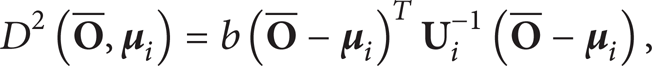
Three run-to-failure tests, test-1 to test-3, have been performed on the test rig. One-second snapshot data were collected at a sampling rate of 20 kHz (20480 samples for each snapshot) every 20 minutes for test-1 and every 10 minutes for test-2 and test-3. At the end of the first run-to-failure experiment a crack was found near the shoulder of bearing-3, while test-2 and test-3 ended up with an outer race defect in bearing-1 and bearing-3, respectively (see Figure 11).

Figure 11:

Damaged bearings [36]. At the end of the first test the bearing-3 experienced a crack near the shoulder (a), while at the end of the second and the third test an outer race defect occurred in bearing-1 (b) and bearing-3 (c), respectively.

In our experiments we considered as training set 4 histories of bearings that did not experience failure (channels X and Y of the first and the second bearing in test-1), and for testing we used the history of a bearing that ended with failure (the third in test-1).

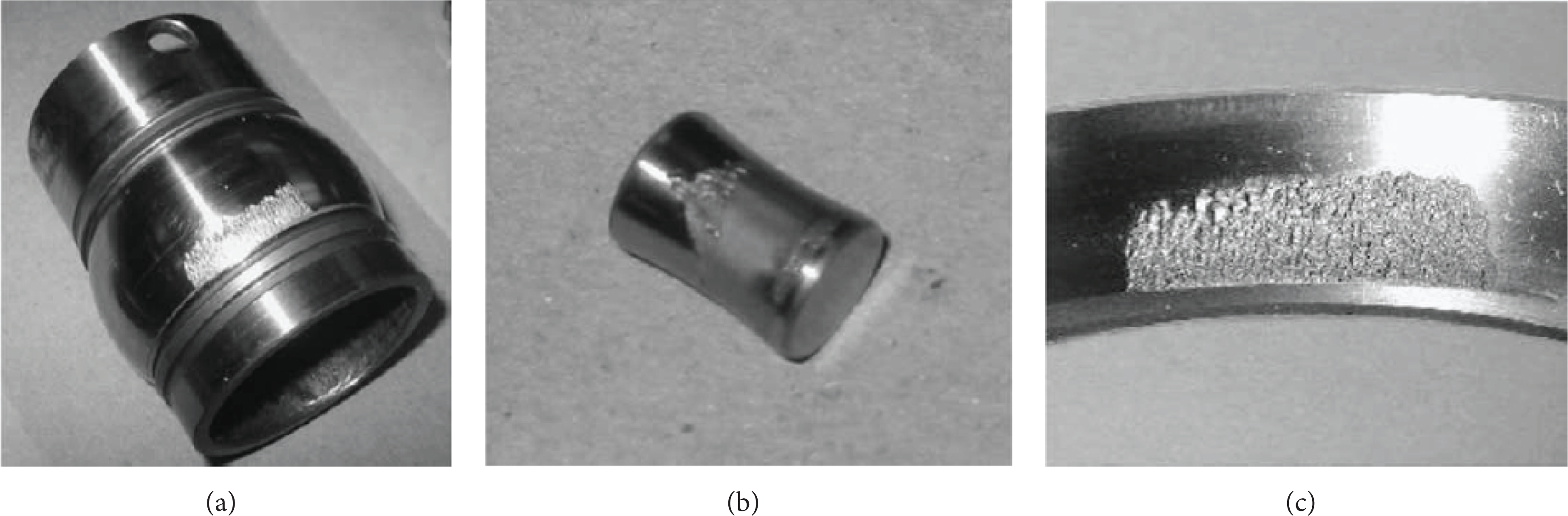
The raw data of the training set have been preprocessed by extracting three time-domain features: mean, root mean square (RMS), and kurtosis within windows of length L = 20480, which is, for simplicity, the same length of the given snapshots. Figure 12 shows the raw vibration data and the resulting RMS signal of length 2156.

Figure 12:

Raw vibration data (a) versus RMS features (b) for bearing-2 in test-1.

4.2.2. Proposed Methodology Results

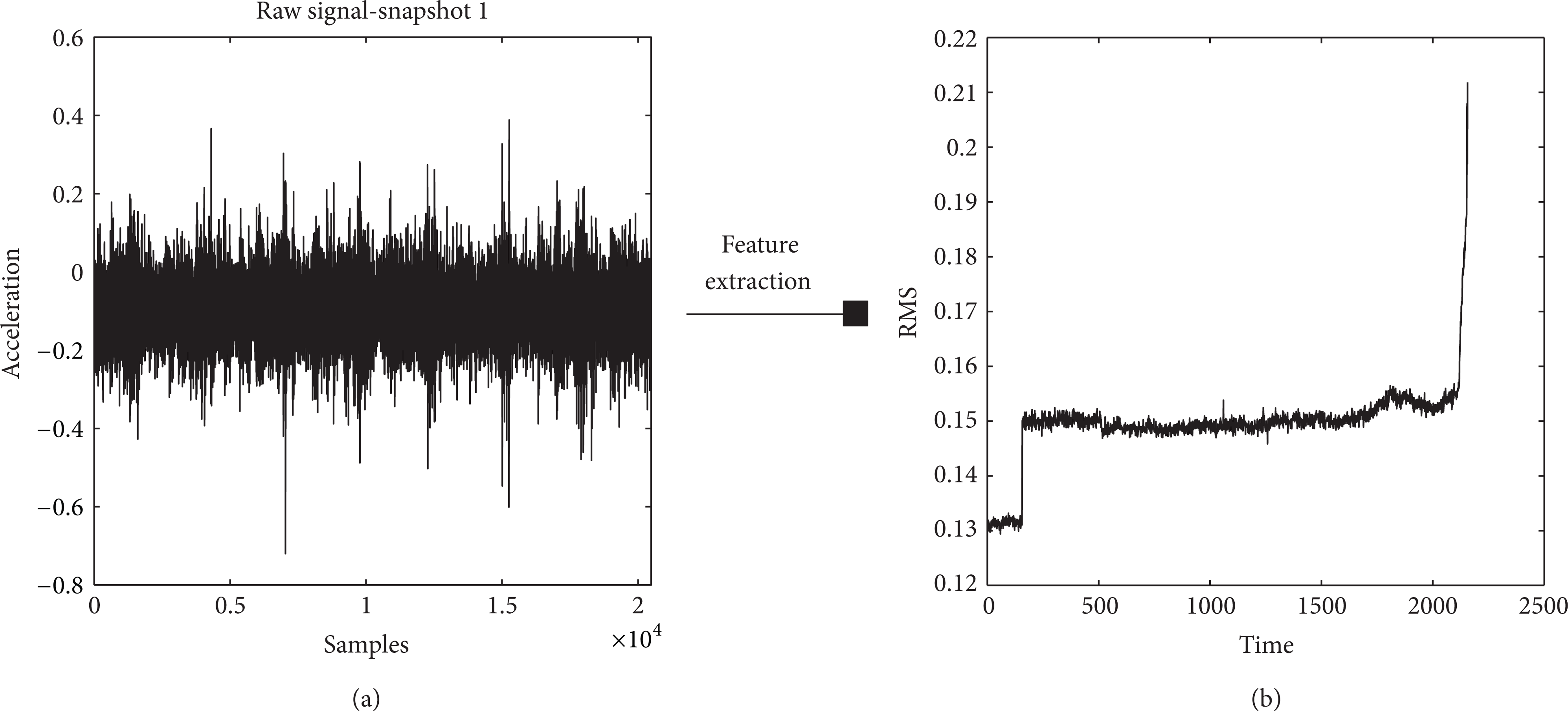
We applied KPCA, with a Gaussian kernel of variance which is equal to 5, to the feature signals. The obtained 1-dimentional signal is illustrated in Figure 13. As it can be seen, the obtained 1-dimensional signal carries the relevant information contained in the three extracted features (mean, RMS, and kurtosis).

Figure 13:

Dimensionality reduction with KPCA on the bearing data.

We then applied the batch CPD algorithm (with a polynomial degree of the fitting function which is equal to 1 and a stability threshold s = 0.03) on the 1-dimensional signal, resulting in the detection of 2 states, as illustrated in Figure 14.

Figure 14:

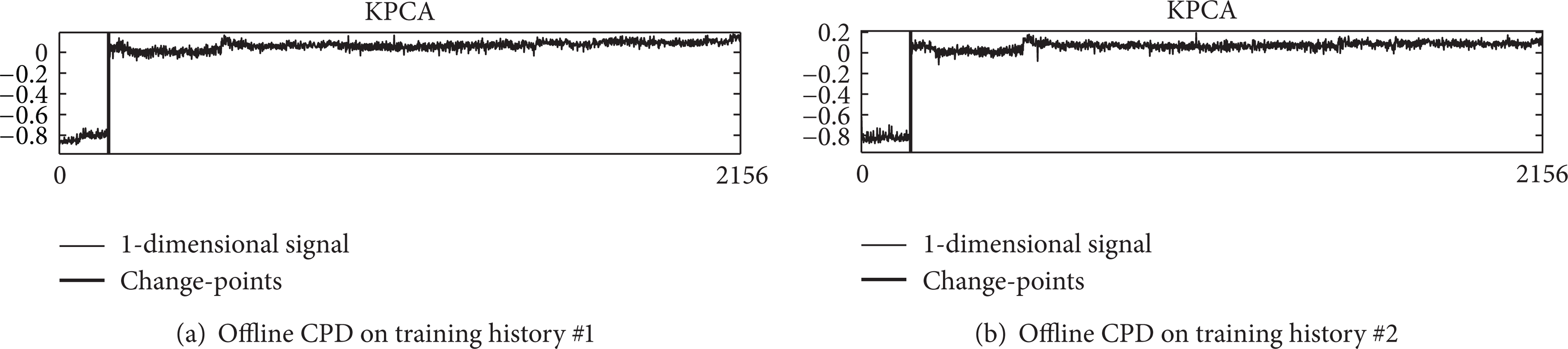
Initial states number estimation with batch CPD for training histories #1 and #2. Two states are detected, also for the third and the fourth training cases.

Since no explicit ground truth about the number of (bearings) states has been made available in the benchmark data [42], we propose using a clustering approach to estimate it. K-means clustering, with varying number of clusters from 2 to 10, has been applied on the (historical) 3-dimensional features observations. The generalized Dunn's validity indexes [28] have been used to determine the optimal number of clusters corresponding to the number of bearing states. Figure 15 illustrates 5 of the 18 validity indexes (V₁₁, …, V₅₁) of [28] versus the number of clusters. High index values indicate the optimal number of clusters, in this case 2. These results confirm that the proposed CPD algorithm applied to the 1-dimensional signal obtained after KPCA dimensionality reduction produces the correct number of bearing states.

Figure 15:

Dunn's validity indexes applied on the 4 training histories.

For the next steps of bearing condition assessment, a 2-state CHMM is considered, for which, as illustrated in Figure 16, the proposed CHMM parameters initialization improves the convergence speed with a final likelihood compared to the value obtained by the best random initialization. For the CHMM observation density, we used a mixture of 3 Gaussians, allowing trade-off between precision and computation time.

Figure 16:

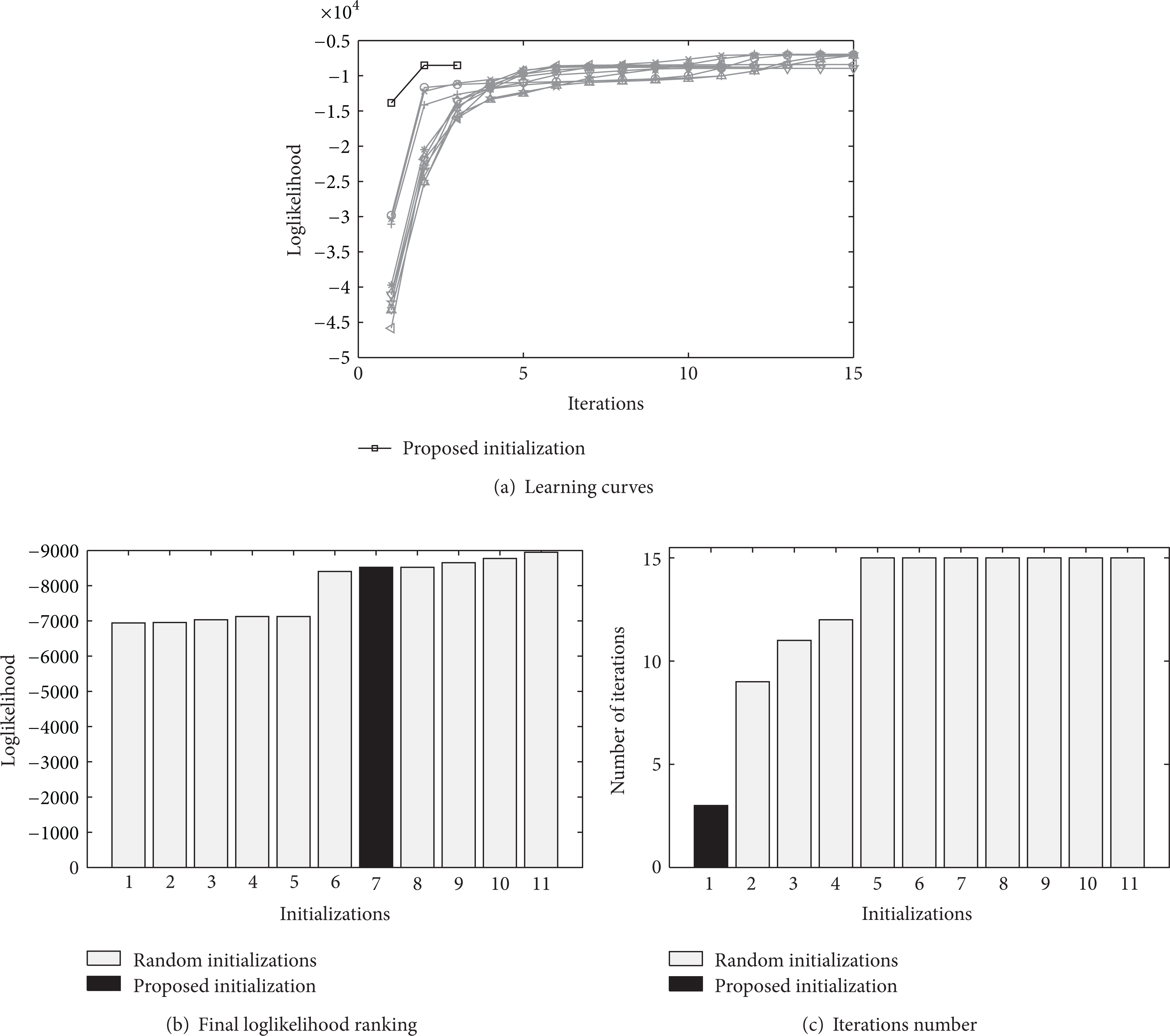
Training Evaluation, the proposed λ₀ estimation versus 10 randomly set λ₀. The effectiveness of the proposed approach for parameters initialization is confirmed in the real case, since the Baum-Welch algorithm converges after only 3 iterations (the fastest in this comparison) and the final likelihood value is comparable with the best random initialization.

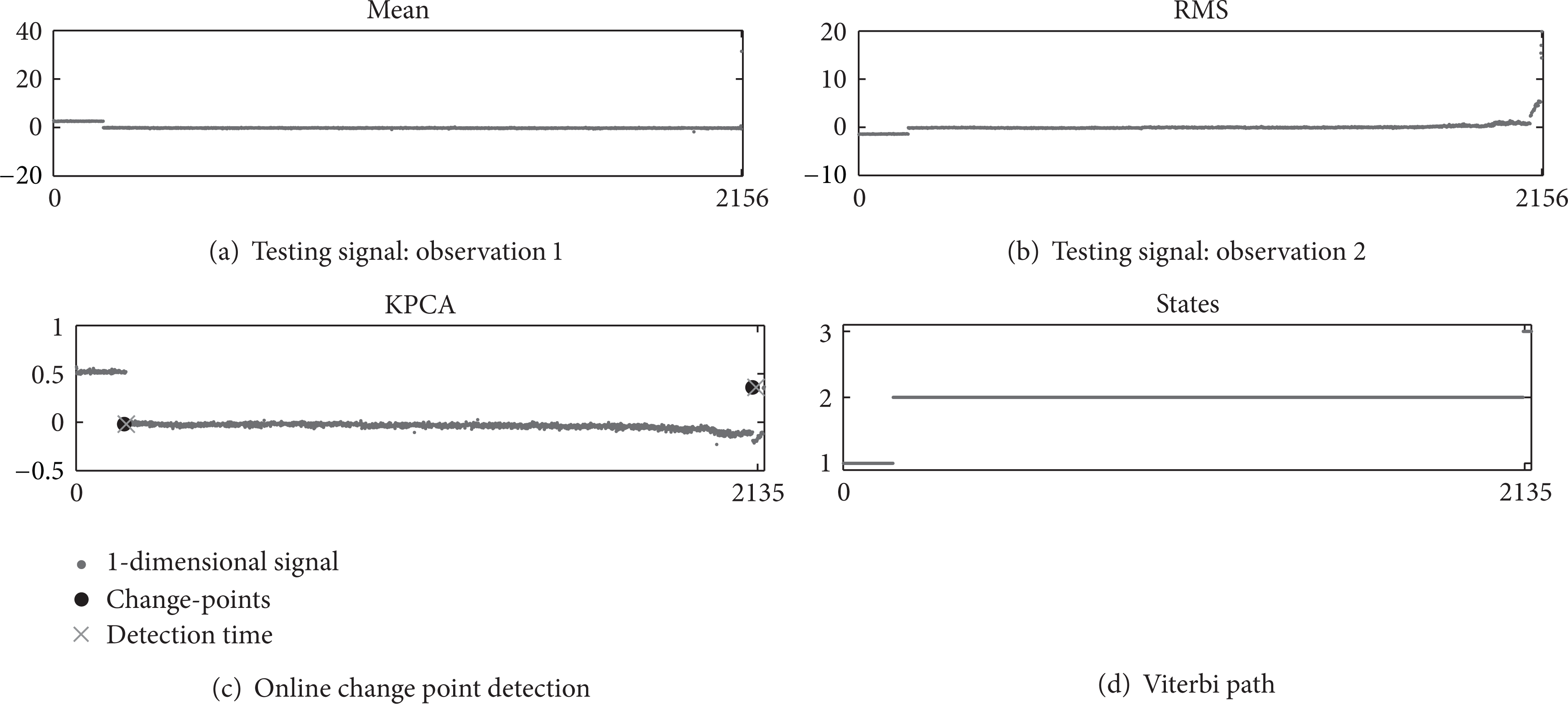
For simulating the online condition assessment using the proposed phase 2 method of Section 3.2, we considered faulty bearing vibration signals to which we applied the feature estimation (mean, RMS, and kurtosis) as described earlier. The resulted features have been successively input to (i) the learned CHMM to calculate the Viterbi path and (ii) to the KPCA dimensionality reduction algorithm for the further application of the online CPD. For the latter, a second degree polynomial fitting function and a threshold δ = 0.6 (equation (15)) have been considered.

The described process above is illustrated in Figure 17. At time 1848, the online CPD correctly detects the beginning of a new degradation modality (Figure 17(d)), which will bring the bearing to fail. A new state is then added to the HMM and the classification of the third state is performed correctly until the end.

Figure 17:

Online condition assessment using the proposed approach. The beginning of a new degradation modality is detected by the online CPD algorithm at an early stage (time 1848), which allowed augmenting the CHMM with a new state. The augmented CHMM correctly detects the degraded state of the bearing (Viterbi path).

From a visual analysis of the observations (see Figure 17), it is clear that the starting of the severe degradation that leads to the bearing failure is reflected by the kurtosis, which at time around 1830 starts to have a discontinuous pattern. This information is correctly captured by the kernel PC and further detected by the online CPD.

4.2.3. Discussion on Features

In this section we discuss different features with the aim of demonstrating that our approach allows determining bearings condition right up until failure and detects the unknown degradation stage at a very early stage, also using different sets of features.

As feature selection is out of the scope of this work, we evaluated the basic state of the art features: mean, RMS, kurtosis, skewness, and wavelet features.

Kurtosis Only. By using only one feature, both the offline and the online CPD algorithms are applied directly on the feature signal itself.

With kurtosis alone, our method fails during the initial state estimation. As can be noticed from Figure 18, the offline CPD algorithm fails to detect the correct point at which a switch between state 1 and state 2 happens for the third and the fourth training histories.

Figure 18:

Initial states number estimation with batch CPD for training histories #3 and #4 based on kurtosis only. The method fails to detect the correct moment in which the state change occurs.

Concerning the online detection of the new state, kurtosis works fine in discovering the bearing degradation at an early stage. In fact, our method detects the unknown condition at sample 1829, 19 samples (6 hours) before the detection using mean, RMS, and kurtosis (see Section 4.2.2). This fact confirms that kurtosis describes well the beginning of the bearing degradation.

However, if we base our method only on the kurtosis, we loose the information about the switch that happens between state 1 and state 2, which is contained in the mean and in the RMS. As can be noticed from Figure 19, both the CHMM and the online CPD agree on the change of condition right at the beginning (sample 8), which is not the case. As a consequence, by using only kurtosis, we fail to determine the correct bearing condition from the beginning to the end.

Figure 19:

Online condition assessment using the proposed approach on kurtosis only. Although the beginning of the bearing degradation is correctly detected at an early stage, kurtosis does not contain the information on the switch from state 1 to state 2 and, consequently, the method fails in determining the correct bearing condition.

Mean and Root Mean Square. By considering only dimensional features like mean and RMS, we obtain the correct results concerning the initial state estimation with offline CPD, as shown in Figure 20.

Figure 20:

Initial states number estimation with batch CPD for training histories #1 and #2 based on mean and RMS. Two states are correctly detected.

However, dimensional features do not contain information about the beginning of the bearing degradation. Hence, the online CPD for the new states detection fails to recognize when the bearing starts to degrade and gives an alert for a new failure condition at sample 2135 (Figure 21). According to the data, it is too late because the bearing is already broken. This is further confirmed from the data description provided by NASA (see Section 4.2.1).

Figure 21:

Online condition assessment using the proposed approach on mean and RMS. The online CPD detects a new failure condition too late, when the bearing is already broken.

We can then conclude that, although combined mean and RMS can determine bearing condition right up until failure, it leads to a late alert of the bearing failure, missing the desirable characteristic of condition monitoring of advising the operator before a catastrophic failure occurs.

Mean, RMS, and Skewness. By substituting skewness to kurtosis and keeping mean and RMS, Figure 22 shows that the offline CPD applied on the KPCA detects the two states of the training bearings, in the same way as it did when using kurtosis (see Section 4.2.2).

Figure 22:

Initial states number estimation with batch CPD for training histories #1 and #2 based on mean, RMS and skewness. Two states are correctly detected.

Concerning the online identification of the new third state, the online CPD takes advantages from skewness in terms of earlier detection of the bearing degradation and slightly outperforms the results obtained in Section 4.2.2. In fact, it detects the third state at sample 1824, 8 hours before.

However, as shown in Figure 23, the Viterbi path of the CHMM fails in detecting the correct state at the end. Hence, we can conclude that, despite the earlier detection of the bearing degradation, the configuration mean, RMS, and skewness is not appropriate to determine bearing condition right up until failure.

Figure 23:

Online condition assessment using the proposed approach on mean, RMS, and skewness. Although The online CPD detects a new failure condition at an early stage, the CHMM fails to assess the correct state sequence at the end.

Wavelet Packet Transform. Finally, we tried our method on time-frequency domain features extracted using the wavelet packet transform (WPT). As described in the work of Pandya et al. [46], we combined the energy and the kurtosis of wavelet coefficients at the second level of the wavelet tree.

Figure 24 shows that offline CPD works fine in detecting the two states of the training bearings, while Figure 25 shows that our methodology detects the new bearing degradation state at sample 1831 when applied on time-frequency features, performing slightly better (around 5 hours earlier detection) than when mean, RMS, and kurtosis are used.

Figure 24:

Initial states number estimation with batch CPD for histories #1 and #2 using the energy and the kurtosis of the second level wavelet packet transform coefficients. Two states are correctly detected.

Figure 25:

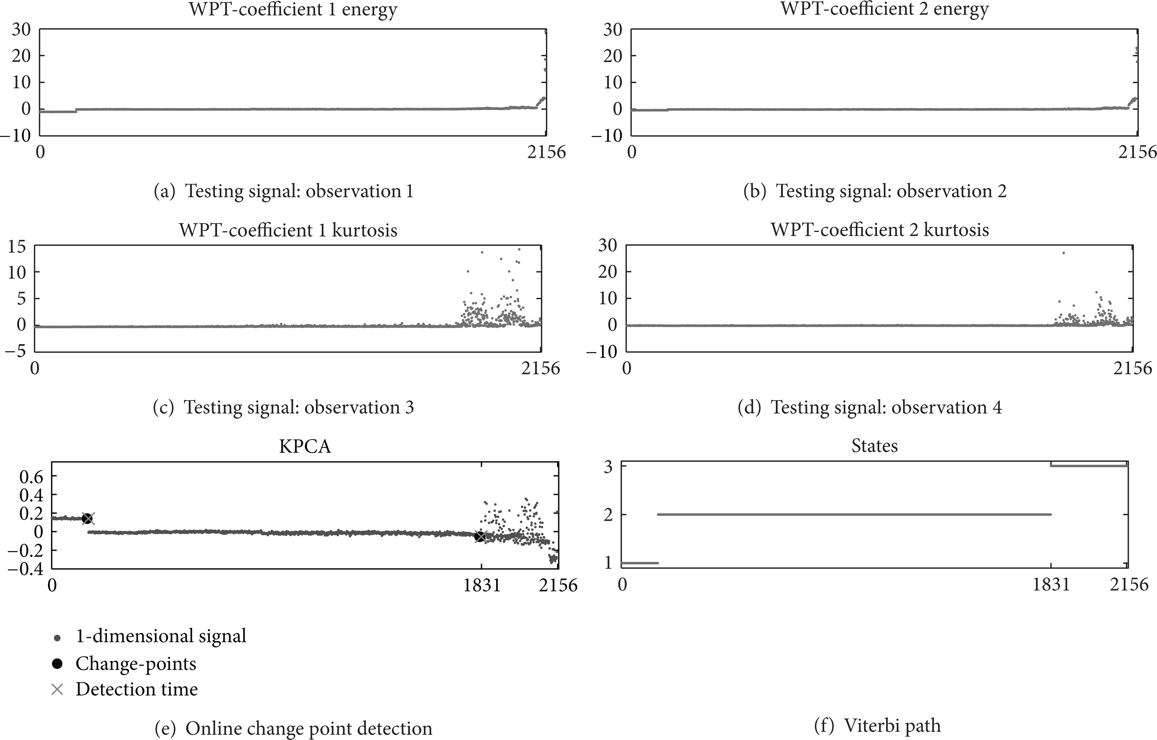
Online condition assessment using the proposed approach on the energy and the kurtosis of WPT tree's second level coefficients. The results obtained with the proposed time domain features are confirmed by using time-frequency domain features.

From the feature study, one can conclude that the proposed mean, RMS, and kurtosis features give good results for condition monitoring of bearings. However, an extended analysis of feature extraction and selection should be made depending on the problem in hand and on the used sensors.

4.2.4. Modified HMM Results

Figure 26 illustrates the approach of Lee et al. [25], in which the detection sensitivity parameter R has been set as R = 6. As it can be seen, the detection of the unknown condition happens at time 2061.

Figure 26:

Online condition assessment using the hotelling multivariate control chart of [25]. The detection of the degradation modality occurs at time 2061 (71 hours later than the proposed approach).

Figure 27, which represents the Mahalanobis distance versus number of sample, illustrates the limits of the approach and its observations modeling, being a joint Gaussian distribution and not a mixture of Gaussians. Hotelling MCC is in fact highly sensitive to small differences between the mean of the testing and the training observation signals. Hence, it is applicable only when training and testing observations are very similar. As demonstrated by the first part of Figure 27, where there are several points out of control at the beginning because the mean of the testing signals in this portion is slightly different from the training set. Although such method would have wrongly detected an unknown situation (a new state would), it has been forced to avoid this behavior by adjusting the parameter R.

Figure 27:

The hotelling multivariate control chart for testing data. The observations modeling through a joint Gaussian distribution is highly sensitive to small differences between the mean of the testing and the training observation signals. Due to this small difference, several out of control points are observed at the beginning, that would have wrongly brought the method to detect an unknown situation.

4.2.5. Discussion

The above results highlight that the proposed methodology

overcomes the limitations imposed by the hotelling MCC since a complex density can be used to model the observations;

is parametric-free; the only parameters are the thresholds of the CPD algorithms, which could be set according to the sensor measurements during the training phase;

is effective in detecting failure modalities at an early stage.

5. Conclusion and Future Work

In this paper, a new approach to the online adaptive condition monitoring has been introduced. The methodology is based on continuous observation hidden Markov models that, combined with the change point detection algorithm, are enhanced to deal with variable state space and are used for condition assessment and unknown state detection. Moreover, a new approach for the HMM initial states number estimation has been provided, together with a method for the parameters initialization. The obtained results illustrate that the proposed methodology (1) correctly estimates the initial number of states for the HMM; (2) improves the execution speed of the training procedure in terms of iterations number reduction with a final likelihood comparable with the best random initialization; (3) classify the current state of the system more effectively than the modified HMM coupled with the hotelling multivariate control chart; (4) detects an anomalous condition or an unknown state at an early stage; and (5) changes the structure and the parameters of the HMM to adapt the model to the new situations.

Our approach has been implemented in Matlab (version 8.3.0), under Windows 7 Enterprise 64-bit Operating System on a desktop computer with an Intel Core i7 3.07 GHz CPU and 16 GB RAM. In terms of computational cost, phase 1, that is, the training phase, takes 296 seconds to learn the CHMM parameters from historical data. It has to be noted that this phase is applied only once for a given machine. Phase 2, that is, the online adaptive condition assessment, takes, on average, 0.2 seconds each time a new snapshot of data is collected (20480 samples). As a consequence, the algorithm can be used in real time condition assessment. In terms of hardware cost, a 164 kBytes buffer is used to store the incoming data, while for the CHMM the memory consumption is proportional to the model structure. In general terms, (N − 1) + (N − 1)·N + D·N·M + D·D·N·M + (M − 1)·N double-precision memory is required, with N the number of states, M the number of Gaussian mixtures in the observation model, and D the number of considered features.

The present work highlights through experiments performed on simulated and real data that the presented methodology can be used in practice as a decision support tool to corrective maintenance strategies. However, it has some problems that must be considered. The dimensionality reduction through kernel principal cmponent analysis causes an inevitable loss of information in the signal used for the change point detection algorithm. To avoid this problem, future researches will consider the application of a modified multidimensional CPD algorithm performed directly in the features hyperplane. Moreover, by using left-right HMMs, it has been assumed that the degradation pattern of the system is characterized by a monotonically increasing evolution which gradually crosses all the wearing phases until the complete failure. Despite being reasonable for bearings, this assumption does not hold for several real systems. In order to render the methodology more generally applicable, it is necessary to consider in future work a method which is able to distinguish also intermediate states and to recognize if the new detected state has been already encountered. Although the present-time researches are oriented to clustering techniques coupled with statistical similarity measures, other methods will be taken into consideration, with the final goal to use as degradation model the more general full ergodic HMM.

Conflict of Interests

The authors declare that there is no conflict of interests regarding the publication of this paper.

References

Honkanen

, Modelling industrial maintenance systems and the effects of automatic condition monitoring [Ph.D. thesis], Helsinki University of Technology, Information and Computer Systems in Automation, Helsinki, Finland, 2004.

Dekker

, “Applications of maintenance optimization models: a review and analysis,” Reliability Engineering & System Safety, vol. 51, no. 3, pp. 229–240, 1996.

Solomon

, “Essential elements of maintenance improvement programs,” in Production Control in the Process Industry: Production Control in the Process Industry No 8: Proceedings of the IFAC Workshop, Osaka, 29–31 and Kariya, Japan, 1–2 Nov. 1989 (Hardback), Oshima

and van Rijn

, Eds., pp. 195–198, Pergamon Press, Oxford, UK, 1989.

Wang

, “A survey of maintenance policies of deteriorating systems,” European Journal of Operational Research, vol. 139, no. 3, pp. 469–489, 2002.

Peng

Dong

, and Zuo

M. J.

, “Current status of machine prognostics in condition-based maintenance: a review,” The International Journal of Advanced Manufacturing Technology, vol. 50, no. 14, pp. 297–313, 2010.

Sfetsos

, “Short-term load forecasting with a hybrid clustering algorithm,” IEE Proceedings: Communications, vol. 150, no. 3, pp. 257–262, 2003.

Vilalta

and Sheng

, “Predicting rare events in temporal domains,” in Proceedings of the 2nd IEEE International Conference on Data Mining (ICDM '02), pp. 474–481, December 2002.

Domeniconi

Perng

C.-S.

Vilalta

, and Ma

, “A classification approach for prediction of target events in temporal sequences,” in Proceedings of the 6th European Conference on Principles of Data Mining and Knowledge Discovery (PKDD '02), pp. 125–137, Springer, London, UK, 2002.

Medjaher

Moya

J.-Y.

, and Zerhouni

, “Failure prognostic by using dynamic Bayesian Networks,” in Dependable Control of Discrete Systems, Fanti

M. P.

and Dotoli

, Eds., vol. 1, IFAC, Bari, Italy, 2009, https://hal.archives-ouvertes.fr/hal-00402938/en/.

10.

Baruah

and Chinnam

R. B.

, “HMMs for diagnostics and prognostics in machining processes,” International Journal of Production Research, vol. 43, no. 6, pp. 1275–1293, 2005.

11.

Zhang

Kwan

Liang

S. Y.

Xie

, and Haynes

, “An integrated approach to bearing fault diagnostics and prognostics,” in Proceedings of the IEEE American Control Conference (ACC '05), vol. 4, pp. 2750–2755, June 2005.

12.

, and Fulei

, “Hidden Markov model-based fault diagnostics method in speed-up and speed-down process for rotating machinery,” Mechanical Systems and Signal Processing, vol. 19, no. 2, pp. 329–339, 2005.

13.

Ertunc

H. M.

Loparo

K. A.

, and Ocak

, “Tool wear condition monitoring in drilling operations using hidden Markov models (HMMs),” International journal of Machine Tools and Manufacture, vol. 41, no. 9, pp. 1363–1384, 2001.

14.

Rabiner

L. R.

, “A tutorial on hidden Markov models and selected applications in speech recognition,” Proceedings of the IEEE, vol. 77, no. 2, pp. 257–286, 1989.

15.

Zhang

, and Borror

C. M.

, “Robustness of the Markov-chain model for cyber-attack detection,” IEEE Transactions on Reliability, vol. 53, no. 1, pp. 116–123, 2004.

16.

Bunks

McCarthy

, and Al-Ani

, “Condition-based maintenance of machines using hidden Markov models,” Mechanical Systems and Signal Processing, vol. 14, no. 4, pp. 597–612, 2000.

17.

Bjerkeseth

, Using hidden markov models for fault diagnostics and prognostics in condition based maintenance systems [Ph.D. dissertation], University of Agder, 2010.

18.

Liu

Chen

, and Dong

, “Application of continuous hide markov model to bearing performance degradation assessment,” in Proceedings of the 24th International Congress on Condition Monitoring and Diagnostics Engineering Management (COMADEM '11), pp. 166–172, 2011.

19.

Ocak

and Loparo

K.A.

, “A new bearing fault detection and diagnosis scheme based on hidden Markov modeling of vibration signals,” in Proceedings of the IEEE Interntional Conference on Acoustics, Speech, and Signal Processing, pp. 3141–3144, IEEE Computer Society, Washington, DC, USA, May 2001.

20.

Almeida

and Park

, “Process monitoring in chemical industries—a hidden Markov model approach,” in Proceedings of the 18th European Symposium on Computer Aided Process Engineering (ESCAPE'18), 2008.

21.

Strachan

and Clifton

, A Hidden Markov Model for Condition Monitoring of a Manufacturing Drilling Process, vol. 1, (IET) Condition Monitoring, Dublin, Ireland, 2009.

22.

Almeida

and Park

, “Fault detection in continuous industrial chemical processes: a new approach using the hidden Markov modeling. Case study: a boiler from a Brazilian cellulose pulp mill,” in Intelligent Data Engineering and Automated Learning—IDEAL 2012, vol. 7435, pp. 743–752, Springer, Berlin, Germany, 2012.

23.

Liu

Chen

Zhou

X. N.

, and Xiao

W.B.

, “Bearing performance degradation assessment using linear discriminant analysis and coupled HMM,” Journal of Physics: Conference Series, vol. 364, no. 1, Article ID 012028, 2012.

24.

Forney

G. D.

Jr. , “The Viterbi algorithm,” Proceedings of the IEEE, vol. 61, pp. 268–278, 1973.

25.

Lee

, and Ni

, “Online degradation assessment and adaptive fault detection using modified hidden markov model,” Journal of Manufacturing Science and Engineering, vol. 132, no. 2, Article ID 021010, 11 pages, 2010.

26.

Cartella

Liu

Meganck

Lemeire

, and Sahli

, “Online adaptive learning of left-right continuous HMM for bearings condition assessment,” Journal of Physics: ConferenceSeries, vol. 364, no. 1, Article ID 012031, 2012.

27.

Guralnik

and Srivastava

, “Event detection from time series data,” Proceedings of the 5th ACM SIGKDD International Conference on Knowledge Discovery and Data Mining (KDD '99), pp. 33–42, 1999.

28.

Bezdek

J. C.

and Pal

N. R.

, “Some new indexes of cluster validity,” IEEE Transactions on Systems, Man, and Cybernetics Part B: Cybernetics, vol. 28, no. 3, pp. 301–315, 1998.

29.

Schölkopf

Smola

, and Müller

K.-R.

, “Nonlinear component analysis as a kernel eigenvalue problem,” Neural Computation, vol. 10, no. 5, pp. 1299–1319, 1998.

30.

Mika

Scholkopf

Smola

Muller

K. R.

Scholz

, and Ratsch

, “Kernel pca and de noising in feature spaces,” in Advances in Neural Information Processing Systems, vol. 11, pp. 536–542, MIT Press, 1999.

31.

Romdhani

Gong

, and Psarrou

, “Amulti-view nonlinear active shape model using kernel pca,” in Proceedings of the British Machine Vision Conference, pp. 483–492, 1999.

32.

O'Donnell

, “Report of large motor reliability survey of industrial and commercial installations, part II,” IEEE Transactions on Industry Applications, vol. 21, no. 4, pp. 865–872, 1985.

33.

J. Q.

and Barron

A. R.

, “Mixture density estimation,” in Advances in Neural Information Processing Systems 12, pp. 279–285, MIT Press, Cambridge, Mass, USA, 1999.

34.

Dempster

A. P.

Laird

N. M.

, and Rubin

D. B.

, “Maximum likelihood from incomplete data via the EM algorithm,” Journal of the Royal Statistical Society B: Methodological, vol. 39, no.1, pp. 1–38, 1977.

35.

Randall

R. B.

, Frequency Analysis, Bruel and Kjaer, 1987.

36.

Qiu

Lee

Lin

, and Yu

, “Wavelet filter-based weak signature detection method and its application on rolling element bearing prognostics,” Journal of Sound and Vibration, vol. 289, no. 4–5, pp. 1066–1090, 2006.

37.

Tobon-Mejia

D. A.

Medjaher

Zerhouni

, and Tripot

, “Estimation of the remaining useful life by using wavelet packet decomposition and hmms,” in Proceedings of the IEEE Aerospace Conference AIAA, pp. 1–10, IEEE Computer Society, Los Alamitos, Calif, USA, 2011.

38.

Burge

and Shaw-Taylor

, “Detecting cellular fraud using adaptive prototypes,” in Proceedings of the AI Approaches to Fraud Detection and Risk Management, pp. 9–13, 1997.

39.

Yamanishi

Takeuchi

Williams

, and Milne

, “Online unsupervised outlier detection using finite mixtures with discounting learning algorithms,” in Proceedings of the 6th ACM SIGKDD International Conference on Knowledge Discovery and Data Mining (KDD '00), pp. 250–254, ACM Press, 2000.

40.

Fawcett

and Provost

, “Activity monitoring: noticing interesting changes in behavior,” in Proceedings of the 5th ACM SIGKDD International Conference on Knowledge Discovery and Data Mining (KDD '99), pp. 53–62, 1999.

41.

Cherkassky

and Mulier

, Learning from Data, Wiley-Interscience, New York, NY, USA, 1998.

42.

NSF-I/UCRC, “Center for intelligent maintenance systems. prognostic data repository: Bearing data set,” http://ti.arc.nasa.gov/tech/dash/pcoe/prognostic-data-repository/.

43.

Tobon-Mejia

D. A.

Medjaher

Zerhouni

, and Tripot

, “A mixture of gaussians hidden markov model for failure diagnostic and prognostic,” in Proceedings of the 6th Annual IEEE International Conference on Automation Science and Engineering (CASE '10), pp. 338–343, IEEE, August 2010.

44.

Tobon-Mejia

D. A.

Medjaher

Zerhouni

, and Tripot

, “Hidden Markov Models for failure diagnostic and prognostic,” in Proceedings of the Prognostics and System Health Management Conference (PHM-Shenzhen '11), pp. 1–8, Shenzhen, China, May 2011.

45.

Tobon-Mejia

D. A.

Medjaher

Zerhouni

, and Tripot

, “A data-driven failure prognostics method based on mixture of gaussians hidden markov models,” IEEE Transactions on Reliability, vol. 61, no. 2, pp. 491–503, 2012.

46.

Pandya

Upadhyay

, and Harsha

S. P.

, “Ann based fault diagnosis of rolling element bearing using time-frequency domain feature,” International Journal of Engineering Science and Technology, vol. 4, pp. 2878–2886, 2012.

Online Adaptive Bearings Condition Assessment Using Continuous Hidden Markov Models

Abstract

1. Introduction

2. Methods and Algorithms

2.1. Left-Right Continuous Hidden Markov Models

2.2. Feature Extraction and Dimensionality Reduction

2.3. Change Point Detection Algorithm

2.3.1. Batch Algorithm

2.3.2. Incremental Algorithm

3. Framework

3.1. Phase 1: Estimation of the Initial Number of States and Parameters Initialization

3.2. Phase 2: Online Adaptive Condition Assessment

4. Experimental Results

4.1. Simulated Experiment

4.1.1. Data Generation

4.1.2. Proposed Approach

4.1.3. Modified HMM Approach [25]

4.1.4. Discussion

4.2. Real Data

4.2.1. Data Description

4.2.2. Proposed Methodology Results

4.2.3. Discussion on Features

4.2.4. Modified HMM Results

4.2.5. Discussion

5. Conclusion and Future Work

Conflict of Interests

References