Identification of Clearance and Contact Stiffness in a Simplified Barrel-Cradle Structure of Artillery System

Abstract

In gun barrel-cradle structure, the presence of clearance usually changes the dynamic response of muzzle and results in shooting dispersion (under continuous firing condition). The parameter estimation of such clearance nonlinear system is the prerequisite for establishing quantitative relation between the clearance and muzzle disturbance. In this paper, the restoring force surface (RFS) method and the nonlinear identification through feedback of outputs (NIFO) method are first combined for parameter identification in a simplified barrel-cradle structure. With the RFS method, clearance value can be obtained by analyzing the restoring force plot. Then the contact stiffness can be identified by using NIFO method. This identification process is verified in a single-degree-of-freedom (SDOF) system with clearance. To adapt to the rigid-flexible coupled beam system with clearances which is simplified from the barrel-cradle structure, a modification for the combined method mentioned above is proposed. The core idea of the modification is reducing the continuous system to multiple-degree-of-freedom (MDOF) system to reserve the nonlinear characteristics through modal transformation matrix. The advantage of this transformation is that the linear parts of the MDOF systems are decoupled, which greatly reduces the difficulty of identification. The simulation results have shown the effectiveness of current method.

1. Introduction

In a large number of engineering structures, clearance always exists due to assemblage, manufacturing errors, and wear [1]. These clearances change dynamic response of the mechanism, cause deviation between theoretical predictions and experimental measurements, and eventually lead to important deviations between the projected behavior of mechanisms and real outcome of mechanisms [2–4]. For the armed forces in each country, the artillery system which is regarded as one of the most important parts in the widely equipped weapon is also greatly troubled by structure gaps. There are different kinds of clearances in the artillery system, such as the clearances in pitch mechanism, the clearances in barrel-cradle structure. These clearances directly lead to muzzle disturbances, which are the key factor affecting shooting dispersion. The quantitative relation between the clearance and muzzle disturbance is very important to improve the firing accuracy in design and practical operation. To establish this relation, the clearance identification and the related contact stiffness identification should first be accomplished. Due to the complexity of artillery system, this paper focuses on the clearances between the barrel and cradle which is more important than others and proposes a combined method to realize the parameter identification of nonlinear systems with clearances.

Since Ibáñez [5] and Masri and Caughey [6] made the first contribution to the identification of nonlinear structural models, many researchers have paid their attention to nonlinear system identification in structural dynamics. The relevant research situation on the methods used in this paper is presented as follows in simplest words. Generally, the existing methods can be divided into seven categories, namely, passing-by nonlinearity: linearization, time and frequency domain methods, modal methods, modal methods, time-frequency analysis, black-box modeling, and structural model updating [7].

The time domain methods employ the vibration signals in the form of time series. The advantage of time domain methods is that data are obtained directly from test equipment and the identification process is simple. The well-known restoring force surface (RFS) method was first proposed by Masri and Caughey [6] in 1979. Kerschen et al. [7] have minutely reviewed the existing methods and showed many productive research achievements. A parallel method named force-state mapping was later independently developed by Crawley et al. [8, 9]. Masri et al. [10] made the generalization to MDOF systems in 1982. Subsequently, an array of researchers, Yang and Ibrahim [11], Al-Hadid and Wright [12–14], Worden [15, 16], Mohammad et al. [17], and Shin and Hammond [18], overcame the series expansion and bias problem as well as numerical computing problem of signals. Various experimental studies published by Audenino et al. [19], Belingardi and Campanile [20], Surace et al. [21], and Kerschen et al. [22] proved that the RFS method was robust. Haroon et al. [23, 24] used the RFS method for nonlinear identification in the absence of input measurement. More recently, Tasbihgoo et al. [25] have utilized polynomial-basis and artificial neural networks, respectively, to identify and represent restoring force.

The frequency domain methods employ the vibration signals in the form of frequency response functions (FRFs) or spectra. The nonlinear identification through feedback of the output (NIFO) formulation [26–28] is a recent spectral approach for identification of MDOF nonlinear systems. It exploits the spatial information and treats the nonlinear forces as internal feedback forces in the underlying linear model of system [7]. Haroon et al. [24] combined the NIFO and RFS methods for nonlinear identification of tire-vehicle suspension system in the absence of input measurements. Spottswood and Allemang [29] extended the method to continuous system by reduced order models. Xie and Mita [30] investigated the underlying linear model of base-isolated structures through NIFO method.

The time-frequency methods do not provide additional insight into the system dynamics compared with combined time- and frequency-domain analyses; they offer a different perspective of the dynamics. Li and Chen [31] summarized the review and classification of the wavelet-based numerical analysis. And a view of the use of the wavelet transform in nonlinear dynamics can be found in [32].

In this paper, considering the structure characteristics of the barrel-cradle system and the feasibility of simulation and experiment, a rigid-flexible coupled beam system with clearance is established as the simplified barrel-cradle model. Then RFS and NIFO methods are combined to conduct the identification on clearance and the related contact stiffness of this model. Moreover, the combined method mentioned above has been improved to make it applicable in modal space. The proposed recognition process was first verified by a SDOF model through simulation and then the effectiveness was verified for the simplified system. Some details related to influencing factors of identification precision are also in this paper.

2. Framework

Virtually all mechanical devices contain several components joined or articulated, at joints which must have some clearance [33]. In most cases, clearance is invisible and sometimes cannot be directly measured. Therefore, some models with clearance should be constructed firstly before the work of identifying nonlinear parameters related to clearance. With this reason, the following will focus on the basic theory of the RFS method and the NIFO method relying on the SDOF system with clearance (Figure 1). This system contains bilateral clearances; the value of d₁ and d₂ can be different. There is contact stiffness k _d between the clearance and the fixed end.

Figure 1:

SDOF system with clearance.

Applying Newton's second law

$m\ddot{x}\left(t\right)+c\dot{x}\left(t\right)+kx\left(t\right)+k_d{U}_d\left[x\left(t\right)\right]=f\left(t\right),$

(1)

where

$U_d\left[x\left(t\right)\right]=\left\{\begin{array}{cc}x\left(t\right)+d_{\mathrm{2}},\hfill & -\infty <x\left(t\right)\le -d_{\mathrm{2}}\hfill \\ \mathrm{0},\hfill & -d_{\mathrm{2}}<x\left(t\right)<d_{\mathrm{1}}\hfill \\ x\left(t\right)-d_1,\hfill & d_1\le x\left(t\right)<\infty .\hfill \end{array}\right.$

(2)

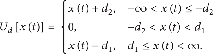
m is the mass of the system, k is the spring stiffness, c is the damping coefficient, f(t) is the applied force, x(t) is the displacement response of the system, k _d U _d [x(t)] is the nonlinear force caused by clearance, where k _d is the equivalent contact stiffness of clearance, and d₁, d₂ are the value of each clearance. The dynamic response of the system can be derived by this second-order nonlinear differential equation. Later the restoring force can be defined as

$f_r\left(x\left(t\right),\dot{x}\left(t\right)\right)=c\dot{x}\left(t\right)+kx\left(t\right)+k_d{U}_d\left[x\left(t\right)\right]=f\left(t\right)-m\ddot{x}\left(t\right)$

(3)

which is a nonlinear function of the displacement and velocity. In addition, the pure nonlinear term f _n (x(t)) = k _d U _d [x(t)] is shown in Figure 2. The turning point in the figure indicates the clearance value and the slope of the line is contact stiffness.

Figure 2:

Pure nonlinear term f _n (x).

2.1. RFS Method

The restoring force can be plotted in a three-dimensional graph against x(t) and $\dot{x}\left(t\right)$ . However, a more suitable representation of the restoring force can be obtained by taking the slice of this three-dimensional plot along the axes where either x(t) or $\dot{x}\left(t\right)$ equals zero [34]. The clearance nonlinearity this paper is interested in is a function that depends on displacement, so just the stiffness curve is needed, and $\dot{x}\left(t\right)$ does not have to be strictly equal to zero for the damping coefficient in the engineering structure we focus on can be usually neglected. What is more, k and c are much less than contact stiffness k _d ; as a result, the linear terms $c\dot{x}\left(t\right)$ and kx(t) contribute a little to restoring force $f_r\left(x\right(t),\dot{x}(t\left)\right)$ . If the restoring force is plotted against displacement, it can well reflect the characteristics of clearance, just as only linear terms do. Then the turning points of the restoring force plot reflect the value of the clearance.

2.2. NIFO Method

The nonlinear identification through feedback of the outputs (NIFO) formulation is an effective method to estimate simultaneously the nonlinear parameters and the linear frequency response function (FRF) matrix throughout the system [27]. This formulation is based on a spatial perspective of the nonlinearity as an internal feedback force [28]. NIFO is a frequency domain identification technique. Applying the Fourier transform to (1), the equation in the frequency domain comes out:

$H_L\left(\omega \right)F\left(\omega \right)-k_d{H}_L\left(\omega \right)F\left[U_d\left(x\left(t\right)\right)\right]=X\left(\omega \right),$

(4)

in which H _L (ω) is the linear FRF, X(ω) and F(ω) are the Fourier transforms of the output x(t), and the F[·] is the Fourier transform operator. Recall that the Fourier transform is based upon the assumption that the signal is a totally observed transient or consists only of harmonics of the time period of observation. Rewrite (4) in the matrix form:

$X\left(\omega \right)=\left[\begin{array}{cc}{H}_L\left(\omega \right)& k_d{H}_L\left(\omega \right)\end{array}\right]\left(\begin{array}{c}F\left(\omega \right)\\ -F\left[U_d\left(x\left(t\right)\right)\right]\end{array}\right).$

(5)

Since the input and output are measured and since the nonlinear function can be calculated explicitly in terms of the measured output, (5) can be used to solve for the best squares estimates of the nonlinear parameter k _d and the linear FRF in a single step, which is not subjected to progressive errors.

We should emphasize that nonlinear characterization should be done before identifying nonlinear parameter using (5). In other words, if the system is not well characterized, the parameter estimation problem is not well-posed because the NIFO formulation involves a correlated source of noise, which produces biased parameter estimates [35]. In this paper, it is very clear that our research goal is clearance nonlinearity. So there is no need for characterization; the author just concentrates on the identification of the clearance value and contact stiffness. But clearance nonlinearity is different from most of other nonlinearities because it cannot be approximated by a mathematical series. The clearance value d does not appear in (2) in the form of coefficient, so clearance identification cannot be accomplished by using NIFO method only. The detailed identification process which is presented to verify the combined method is shown in Figure 3.

Figure 3:

Flow chart of recognition process.

As shown in Figure 3, there are three main steps for estimating the parameters in a SDOF system with clearance.

(1) Construct an Appropriate Model. In order to carry out the identification process, the corresponding mathematical model should be established to obtain the dynamic response.

(2) Identify the Value of Clearance through RFS Method. The clearance value should be identified firstly, because the clearance value is used in identification of contact stiffness. When the dynamic response of model is known, the clearance can be estimated immediately by the RFS method. Then check the identification; if the error is not within allowed error, the method should be examined or modified if necessary.

(3) Identify the Contact Stiffness Using NIFO Method. After identifying the value of clearance, the contact stiffness can be identified using the NIFO method. Then check the identification; if the error is not within allowed error, the method should be examined or modified if necessary.

2.3. Study of SDOF System

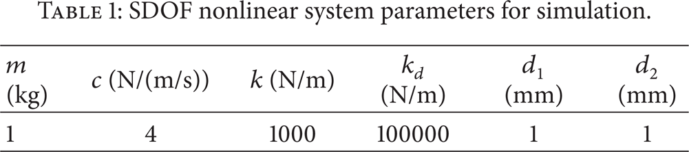
A SDOF system is shown in Figure 1, and the parameters of this system are given in Table 1. As discussed above, the clearance value is identified with the help of the restoring force against displacement x(t). The Gaussian inputs were chosen to excite both the linear model and the nonlinear model with clearance (the amplitudes of inputs are the same). The outputs of each system are shown in Figure 4. It is obvious that the existence of clearance limits the amplitude of displacement and makes the response signals more confusing. The restoring force is plotted against displacement x(t) and velocity $\dot{x}\left(t\right)$ in Figure 5, and Figure 6 shows the plot of restoring force against displacement x(t), which displays typical clearance nonlinearity. The abscissa of the turning point is the clearance value.

Table 1:

SDOF nonlinear system parameters for simulation.

m (kg)	c (N/(m/s))	k (N/m)	k d (N/m)	d1 (mm)	d2 (mm)
1	4	1000	100000	1	1

Figure 4:

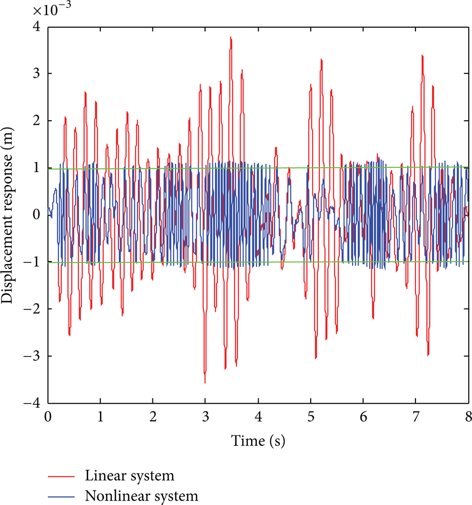
Outputs of linear SDOF system and nonlinear system with clearance.

Figure 5:

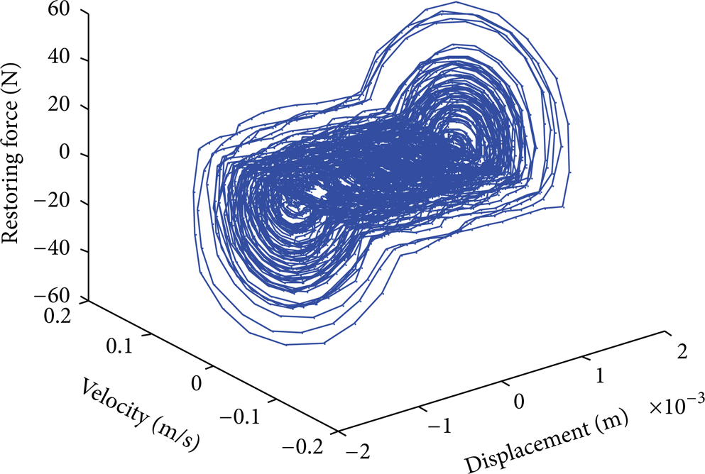
Restoring force $f_r\left(x\right(t),\dot{x}(t\left)\right)$ plot against x(t) and $\dot{x}\left(t\right)$ .

Figure 6:

Restoring force f _r (x(t)) plot against x(t).

However, Figure 6 is not as ideal as Figure 5, because there are thousands of turning points gathering around the true clearance value. In order to fit curves for restoring force surface, the software package Europe was used in Figure 7. The goal of the software package is to identify the simplest mathematical formulas which could describe the underlying mechanisms that produced the data [36]. The final result is expressed as

$y=\min \left[\max \left(101000x-\mathrm{100,997.5}x\right),100.1\right.\left.+101100x\right].$

(6)

Figure 7:

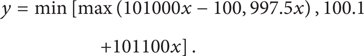
Restoring force f _r (x(t)) plot against x(t) plotted by Eurepa.

In Figure 7, the abscissas of the turning points are −0.001 and 0.001 apparently, which means the clearance is symmetrical and the clearance value is 0.001 m.

The linear parameter in (5) is H _L (ω), the FRF of the underlying linear system, and the nonlinear parameter is k _d . In this example k _d is constant; however, nonlinear parameters that vary with frequency can also be estimated. The nonlinear parameters and the FRF of the underlying linear system were estimated by writing (5) N times, where N was the number of averages, and solving the resulting set of equations using least squares techniques. The simulation was implemented in the commercial software package MATLAB. The following parameters were used in the solution of (5): 40 averages, a Hanning Window, 50% overlap, and a block size of 25000. In order to separate the clearance nonlinear from system, the clearance should be about 15% of the total Root-Mean-Square (RMS) value of the corresponding linear forces. Therefore amplitudes of the band limited Gaussian inputs were chosen to make nonlinear forces. If the SDOF system shown in Figure 2 had no clearance nonlinearity, the natural frequency of the SDOF system should be around 5 Hz. So the frequency range was chosen between 0 and 15 Hz.

The results are shown in Figures 8 and 9. Figure 8 displays the estimated contact stiffness k _d . Notice that the contact stiffness is very nearly independent of frequency, which is consistent with the assumed parameter above. The spectral mean of this estimate is 0.048% total RMS error of the true parameter in the interested frequency band. The upper and lower plots in Figure 9 show the magnitude and phase of two FRFs, respectively. The true FRF of the linear system is drawn with a solid line and the estimate of the linear FRF with a dotted line. Note that the estimate FRF matches well the true linear system FRF with a total squared error down to 0.5% in the view of both magnitude and phase.

Figure 8:

SDOF system estimation: (a) estimation of contact stiffness k _d , (b) estimation error.

Figure 9:

Magnitude and phase of the FRFs of the SDOF system with clearance (solid line: linear FRF; dotted linear: estimated FRF of linear system).

3. Modified RFS and NIFO Methods for Barrel-Cradle Structure with Clearance

3.1. Reduced Model of Barrel-Cradle Structure with Clearance

Barrel and cradle are two important parts of artillery system. The shape of the cradle determines how barrel is connected to the cradle. U-type cradle and composite cradle both have U-type frame and sliding guide. The sliding guides of the cradle and sliding slot on the barrel fit together to guide the recoiling and counter-recoiling rectilinear movement of the barrel. There is assembling clearance between the sliding guides and the sliding slot to ensure smooth sliding. The existence of clearance will have a significant impact on the dynamic response of artillery systems and then will affect firing accuracy and dispersion. Two key parameters, the clearance value and the contact stiffness, play an important role in the artillery system design. As mentioned in Section 2, three steps were established to identify the clearance value and the contact stiffness of the artillery systems. (1) Construct a simplified model of the fit of the sliding guides and the sliding with clearance. (2) Identify the clearance value through improved RFS method. (3) Identify the contact stiffness using improved NIFO method.

In order to obtain a general model, many details of barrel and cradle structure in an artillery system are neglected and some assumptions are made for ease of calculation. The reduced model named rigid-flexible coupled beam system with clearance is shown in Figure 10, in which beam 1 represents the cradle and beam 2 represents the barrel. Beam 1 is a cantilever with left end fixed and beam 2 is a beam free from any constraints. It is noticed that the influence of the material deformation on mechanical motion is very important [37]. So here the gravity is ignored for it will influence the shape of beam 2 seriously which makes more differences from the barrel-candle structure (due to the different moments of inertia). Beam 2 is driven by an applied force as system excitation. The displacement response of the beams is represented by the absolute displacements u(x₁, t) and v(x₂, t). The model is defined by the following parameters: beam length l _i (i = 1,2), cross-sectional areas A _i (i = 1,2), cross-sectional moments of inertia I _i (i = 1,2), density ρ and Young's modulus E of the two flexible parts, and the distance between left point of the two beams l _a (t). The contact between the beams is realized via discrete spring-damper systems in the form of so-called displacement condition (not a force condition) [38], the clearances d₁, d₂, the contact stiffness k _d , and damping coefficient c that are shown in Figure 9.

Figure 10:

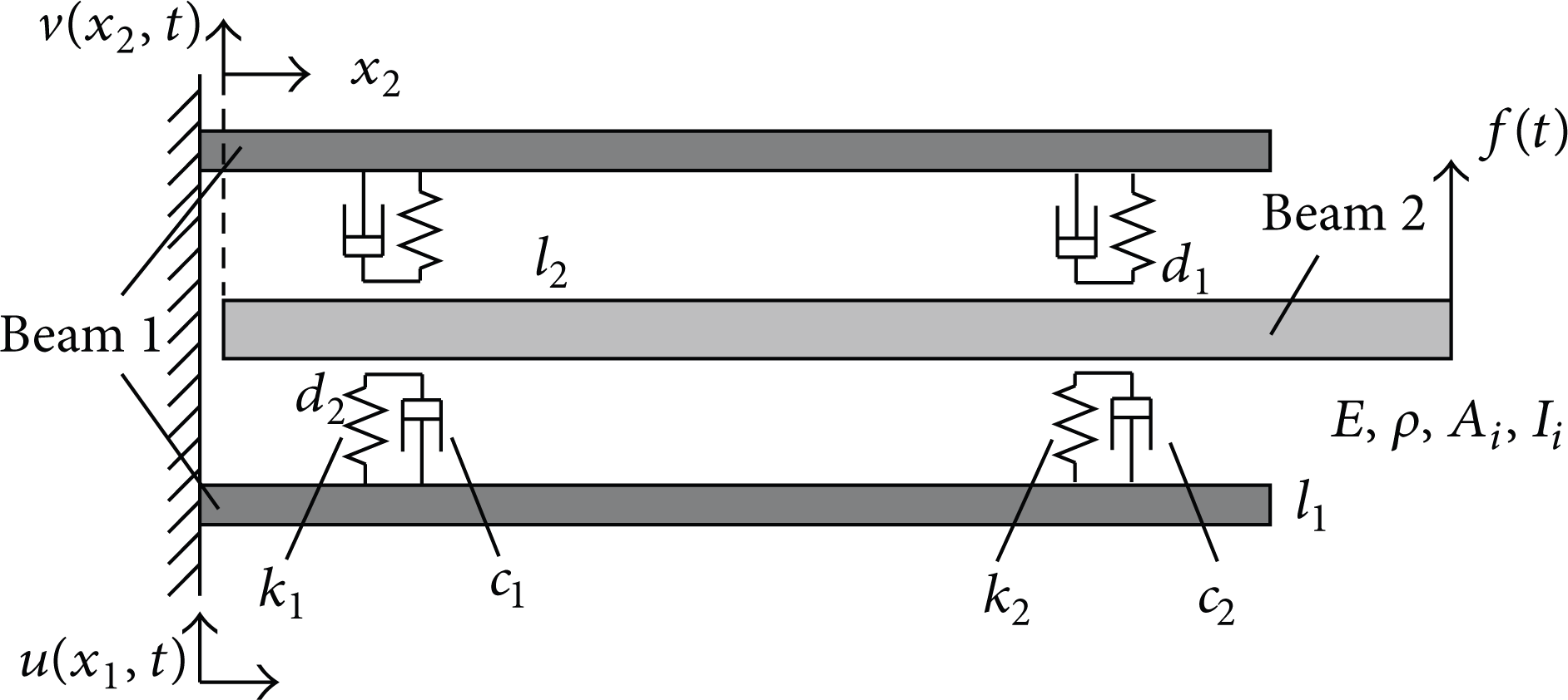
Simplified model: rigid-flexible coupling Euler beam model with clearance.

Applying Hamilton's principle

$\delta {{\displaystyle \int }}_{t_0}^{t_1}\left(T-U\right)\text{d}t+{{\displaystyle \int }}_{t_0}^{t_1}{W}_{\text{virt}}\text{d}t=0$

(7)

the governing boundary value problem can be derived. T is the kinetic energy, U is the potential energy, and W_virt is the virtual work of forces without potential of the considered system and t₁ and t₀ are the beginning and the end of time, respectively. When beam segments of uniform cross-sectional properties ρA₁, ρA₂, EI₁, and EI₂ are assumed, the kinetic energy can be written as

$T=\frac{1}{2}{{\displaystyle \int }}_0^{l_1}\rho A_1{u}_t^2\text{d}{x}_1+\frac{1}{2}{{\displaystyle \int }}_0^{l_2}\rho A_2{v}_t^2\text{d}{x}_2.$

(8)

If the action of the spring-damper systems is completely included into the virtual work, for the remaining potential energy one obtains

$U=\frac{1}{2}{{\displaystyle \int }}_0^{l_1}E{I}_1{u}_{x_1{x}_1}^2\text{d}{x}_1+\frac{1}{2}{{\displaystyle \int }}_0^{l_2}E{I}_2{v}_{x_2{x}_2}^2\text{d}{x}_2.$

(9)

The virtual work contains all the contact forces between the beams and the applied force on beam 2 which couple with the resulting field equation:

$W_{\text{virt}}={{\displaystyle \int }}_0^{l_1}{f}_1\delta w\hspace{0.17em}\text{d}{x}_1+{{\displaystyle \int }}_0^{l_2}{f}_2\delta v\hspace{0.17em}\text{d}{x}_2.$

(10)

Evaluating Hamilton's principle (7) by introducing T, U, and W_virt according to (8)–(10), respectively, we obtain the governing field equations

$\begin{array}{c}\rho A_1{u}_{tt}+E{I}_1{u}_{x_1{x}_1{x}_1{x}_1}=f_1\left(x_1,t\right)\\ \rho A_2{v}_{tt}+E{I}_2{v}_{x_2{x}_2{x}_2{x}_2}=f_2\left(x_2,t\right).\end{array}$

(11)

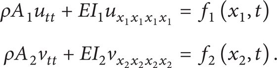
The corresponding boundary conditions are as follows:

$\begin{array}{c}u\left(0,t\right)=0,\\ u_{x_1}\left(0,t\right)=0,\\ u_{x_1{x}_1}\left(l_1,t\right)=0,\\ u_{x_1{x}_1{x}_1}\left(l_1,t\right)=0,\\ v_{x_2{x}_2}\left(0,t\right)=0,\\ v_{x_2{x}_2{x}_2}\left(0,t\right)=0,\\ v_{x_2{x}_2}\left(l_2,t\right)=0,\\ v_{x_2{x}_2{x}_2}\left(l_2,t\right)=0.\end{array}$

(12)

The two beams contact each other at the two points x₁ = l₁ and x₂ = 0 only, representing the interaction between the sliding guides and the sliding slot with a simple case. The concentrated forces are specified as

$\begin{array}{c}{f}_{\mathrm{1}}=-\delta \left(x_{\mathrm{1}}-l_a\right)\left[F_k\left({\eta }_{\mathrm{1}}\left(t\right)\right)+\frac{\text{d}}{\text{d}t}{\eta }_{\mathrm{1}}\left(t\right)·F_c\left({\eta }_{\mathrm{1}}\left(t\right)\right)\right]-\delta \left(x_{\mathrm{1}}-l_{\mathrm{1}}\right)\left[F_k\left({\eta }_{\mathrm{2}}\left(t\right)\right)+\frac{\text{d}}{\text{d}t}{\eta }_{\mathrm{2}}\left(t\right)·F_c\left({\eta }_{\mathrm{2}}\left(t\right)\right)\right],\\ f_2=\delta \left(x_2-\left(l_1-l_a\right)\right)\left[F_k\left({\eta }_2\left(t\right)\right)+\frac{\text{d}}{\text{d}t}{\eta }_2\left(t\right)·F_c\left({\eta }_2\left(t\right)\right)\right]+\delta \left(x_2\right)\left[F_k\left({\eta }_1\left(t\right)\right)+\frac{\text{d}}{\text{d}t}{\eta }_1\left(t\right)·F_c\left({\eta }_1\left(t\right)\right)\right]+\delta \left(x_2-l_2\right)F\left(t\right),\end{array}$

(13)

where

$\begin{array}{c}{F}_k\left(\eta \left(t\right)\right)=k\left[\eta \left(t\right)-\frac{1}{2}\left(\eta \left(t\right)+\frac{l_s}{2}\right)\mathrm{sign}\left(\eta \left(t\right)+\frac{l_s}{2}\right)\right.+\left.\frac{1}{2}\left(\eta \left(t\right)-\frac{l_s}{2}\right)\mathrm{sign}\left(\eta \left(t\right)-\frac{l_s}{2}\right)\right],\\ F_c\left(\eta \left(t\right)\right)=c\left[1-\frac{1}{2}\mathrm{sign}\left(\eta \left(t\right)+\frac{l_s}{2}\right)+\frac{1}{2}\mathrm{sign}\left(\eta \left(t\right)-\frac{l_s}{2}\right)\right],\\ {\eta }_1\left(t\right)=v\left(0,t\right)-u\left(l_a\left(t\right),t\right),\\ {\eta }_2\left(t\right)=v\left(\left(l_1-l_a\left(t\right)\right),t\right)-u\left(l_1,t\right).\end{array}$

(14)

The characteristic of F _k (η(t)) is just the same as shown in Figure 2. Figure 11 shows the damping force F _c (η(t)) versus the relative position η(t) of the contact points. Figures 2 and 11 show the fact that no forces can be transferred in the range of backlash.

Figure 11:

Damping characteristic F _c (η(t)).

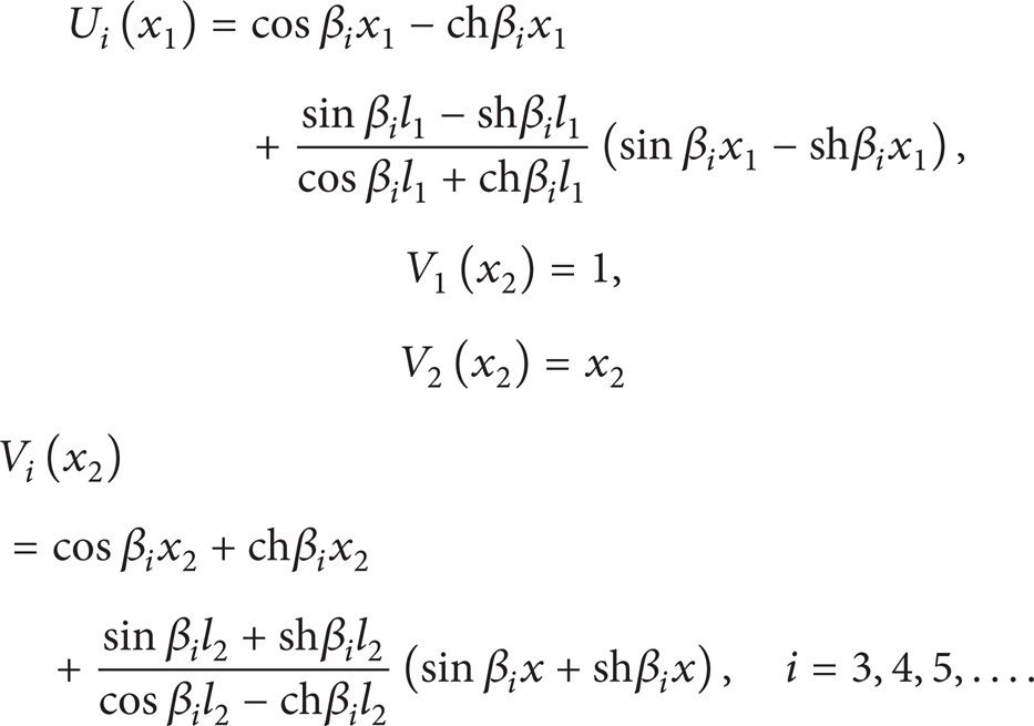
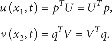
An assumed mode method is used to investigate the coupled partial differential equations (11) together with the corresponding boundary conditions (12). The approximate solutions u(x₁, t) and v(x₂, t) are represented by a series expansion using selected shape functions U _i (x₁) and V _i (x₂) (i = 1,2, …, N) fulfilling all boundary conditions (12):

$\begin{array}{c}u\left(x_{\mathrm{1}},t\right)={\displaystyle \sum }_{i=\mathrm{1}}^n{U}_i\left(x_{\mathrm{1}}\right)p_i\left(t\right)\\ v\left(x_2,t\right)={\displaystyle \sum }_{i=1}^n{V}_i\left(x_2\right)q_i\left(t\right),\end{array}$

(15)

where U _i (x₁) and V _i (x₂) are assumed modes and p _i (t) and q _i (t) are generalized or modal coordinates. The shape functions U _i (x₁) and V _i (x₂) which meet the boundary conditions are specified as

$\begin{array}{c}{U}_i\left(x_1\right)=\cos {\beta }_i{x}_1-\text{ch}{\beta }_i{x}_1+\frac{\sin {\beta }_i{l}_1-\text{sh}{\beta }_i{l}_1}{\cos {\beta }_i{l}_1+\text{ch}{\beta }_i{l}_1}\left(\sin {\beta }_i{x}_1-\text{sh}{\beta }_i{x}_1\right),\\ V_1\left(x_2\right)=1,\\ V_2\left(x_2\right)=x_2\\ V_i\left(x_2\right)=\cos {\beta }_i{x}_2+\text{ch}{\beta }_i{x}_2\hspace{1em}+\frac{\sin {\beta }_i{l}_2+\text{sh}{\beta }_i{l}_2}{\cos {\beta }_i{l}_2-\text{ch}{\beta }_i{l}_2}\left(\sin {\beta }_{i}x+\text{sh}{\beta }_{i}x\right),\hspace{1em}i=\mathrm{3,4},5,\dots .\end{array}$

(16)

Assume that

$\begin{array}{c}U={\left[\begin{array}{cccc}{U}_1\left(x_1\right)& U_2\left(x_1\right)& \cdots & U_n\left(x_1\right)\end{array}\right]}^T,\\ V={\left[\begin{array}{cccc}{V}_1\left(x_2\right)& V_2\left(x_2\right)& \cdots & V_n\left(x_2\right)\end{array}\right]}^T,\\ p={\left[\begin{array}{cccc}{p}_1\left(t\right)& p_2\left(t\right)& \cdots & p_n\left(t\right)\end{array}\right]}^T,\\ q={\left[\begin{array}{cccc}{q}_1\left(t\right)& q_2\left(t\right)& \cdots & q_n\left(t\right)\end{array}\right]}^T.\end{array}$

(17)

The displacement response can be written as

$\begin{array}{c}u\left(x_1,t\right)=p^{T}U=U^{T}p,\\ v\left(x_2,t\right)=q^{T}V=V^{T}q.\end{array}$

(18)

Further, taking the four-mode expansion as an example, the author should consider the translational mode and rotational mode to express rigid motion of beam 2. For each beam, there are four equations describing the approximate vibration response. A total of eight equations coupled together represent the above system. The relative displacements at the contact points η₁(t), η₂(t) are function of p _i (t) and q _i (t), so the nonlinear forces caused by clearance are also function of p _i (t) and q _i (t); as a result, the eight equations are coupled together:

$\begin{array}{c}{m}_{\mathrm{1}i}{\ddot{p}}_i+c_{\mathrm{1}i}{\dot{p}}_i+k_{\mathrm{1}i}{p}_i-U_i\left(l_a\right)F_{k\mathrm{1}}\left(t\right)-U_i\left(l_{\mathrm{1}}\right)F_{k\mathrm{2}}\left(t\right)=\mathrm{0},\hspace{1em}\left(i=\mathrm{1,2},\mathrm{3,4}\right),\\ m_{2i}{\ddot{q}}_i+c_{2i}{\dot{q}}_i+k_{2i}{q}_i+V_i\left(0\right)F_{k1}\left(t\right)+V_i\left(l_1-l_a\right)F_{k2}\left(t\right)=V_i\left(l_2\right)F\left(t\right),\hspace{1em}\left(i=\mathrm{1,2},\mathrm{3,4}\right).\end{array}$

(19)

3.2. Modified RFS Method

To apply the RFS method to the nonlinear system in Figure 9, (19) should be resorted to for drawing the restoring force curve against displacement response. Because the displacements at each point on beam system will disturb each other and appear as chaos phenomenon, if the displacement and acceleration response at the right end of the beam 2 are measured, and the measured results are applied into (3), the obtained restoring force plot against displacement could not represent the feature of clearance nonlinearity. The signals measured at different locations should be transformed into modal space. Since the first four mode shapes are taken into consideration, at least four gauging points should be deployed to each beam. Once the acceleration response ${\ddot{q}}_i$ and displacement response q _i in the ith-order are known, the restoring force can be calculated by

$F_{r2i}=c_{2i}{\dot{q}}_i+k_{2i}{q}_i+V_i\left(0\right)F_{k1}\left(t\right)+V_i\left(l_1-l_a\right)F_{k2}\left(t\right)=V_i\left(l_2\right)F\left(t\right)-m_{2i}{\ddot{q}}_i.$

(20)

The nonlinear terms are functions of the relative displacements at the contact point, so the abscissa in the restoring force plot should be η₁(t), η₂(t). Instead of having only one nonlinear term like (3), there are two nonlinear terms in (20). Under the actual situation, only the sum of the two nonlinear forces can be obtained. The characteristics of the two nonlinear terms are similar; they have the same turning point. The restoring force plot may not be as clear as Figure 6, so the relative displacements η₁(t), η₂(t) should be taken into consideration. The statistics of the occurrence of relative displacements η₁(t), η₂(t) can be regarded as good indexes to estimate clearance value, and the estimating result can be verified in the previous restoring force plot.

3.3. Modified NIFO Method

The method introduced here is based upon the NIFO method, and the continuous system is reduced to MDOF system through modal transformation matrix with nonlinear characteristics totally reserved. The advantage of this transformation is that the linear parts of the MDOF systems are decoupled, which greatly reduces the difficulty of the identification.

In order to apply NIFO method to rigid-flexible coupled beam system with clearance, the first sixteen modes are used to approach the displacement response of this system. However, for the sake of easy identification, the vibration response signal in the physical space should be transformed to the modal space that consists of first four modes. The transformation is expressed as

$\begin{array}{c}\left\{p\left(t\right)\right\}={\left[U_{\mathrm{trans}}\right]}^{-1}\left\{x_1\left(t\right)\right\},\\ \left\{q\left(t\right)\right\}={\left[V_{\mathrm{trans}}\right]}^{-1}\left\{x_2\left(t\right)\right\},\end{array}$

(21)

where U_{trans ⁡} and V_{trans ⁡} are transformation matrices and each column represents the values of a particular modal function at different measuring points. Then the measured data can be transformed into modal space.

Applying the Fourier transform to (19) frequency-domain equations come out

$-{\omega }^{\mathrm{2}}{m}_{\mathrm{1}i}{P}_i\left(\omega \right)+j\omega c_{\mathrm{1}i}{P}_i\left(\omega \right)+k_{\mathrm{1}i}{P}_i\left(\omega \right)-U_i\left(l_a\right)F_{k\mathrm{1}}\left(\omega \right)-U_i\left(l_{\mathrm{1}}\right)F_{k\mathrm{2}}\left(\omega \right)=\mathrm{0},\hspace{1em}\left(i=\mathrm{1,2},\mathrm{3,4}\right),$

(22)

$-{\omega }^2{m}_{2i}{Q}_i\left(\omega \right)+j\omega c_{2i}{Q}_i\left(\omega \right)+k_{2i}{Q}_i\left(\omega \right)+V_i\left(0\right)F_{k1}\left(\omega \right)+V_i\left(l_1-l_a\right)F_{k2}\left(\omega \right)=V_i\left(l_2\right)F\left(\omega \right),\hspace{1em}\left(i=\mathrm{1,2},\mathrm{3,4}\right),$

(23)

where P _i (ω) is the ith modal coordinate in the frequency domain, F(ω) is the modal force in the frequency domain, and F_k1(ω) and F_k2(ω) represent the nonlinear modal coupling terms transformed into the frequency domain. Recall that the Fourier transform is based upon the assumption that the signal is a totally observed transient or consists solely of harmonics of the time period of observation. Using the system normal modes in the transformation from physical space to the modal space, the linear terms are uncoupled, while nonlinear terms remain coupled. As each of the eight equations has nonlinear terms caused by clearance, the NIFO method can be applied to each equation.

Assume that

$\begin{array}{c}{F}_{k\mathrm{1}}\left(\omega \right)=k_{d\mathrm{1}}{U}_{d\mathrm{1}}\left(\omega \right),\\ F_{k2}\left(\omega \right)=k_{d2}{U}_{d2}\left(\omega \right).\end{array}$

(24)

Then (23) can be written as

$k_{d1}\left(\omega \right)H_{2i}\left(\omega \right){\tilde{U}}_{di}\left(\omega \right)+k_{d2}\left(\omega \right)H_{2i}\left(\omega \right){\tilde{U}}_{d2}\left(\omega \right)+H_{2i}\left(\omega \right)\tilde{F}\left(\omega \right)=X_{2i}\left(\omega \right),$

(25)

where

$\begin{array}{c}{\tilde{U}}_{d1}\left(\omega \right)=V_i\left(0\right)U_{d1}\left(\omega \right),\\ {\tilde{U}}_{d2}\left(\omega \right)=V_i\left(l_1-l_a\right)U_{d2}\left(\omega \right),\\ H_{2i}\left(\omega \right)=\frac{1}{-m_{2i}{\omega }^2+j\omega c_{2i}+k_{2i}},\\ \tilde{F}\left(\omega \right)=V_i\left(l_2\right)F\left(\omega \right).\end{array}$

(26)

Assume that

$\begin{array}{c}B=\left[\begin{array}{ccc}\tilde{F}\left(\omega \right)& {\tilde{U}}_{d1}\left(\omega \right)& {\tilde{U}}_{d2}\left(\omega \right)\end{array}\right]\hfill \\ b={\left[\begin{array}{ccc}{H}_{2i}\left(\omega \right)& k_{d1}\left(\omega \right)H_{2i}\left(\omega \right)& k_{d2}\left(\omega \right)H_{2i}\left(\omega \right)\end{array}\right]}^T\\ x=X_{2i}\left(\omega \right),\hfill \end{array}$

(27)

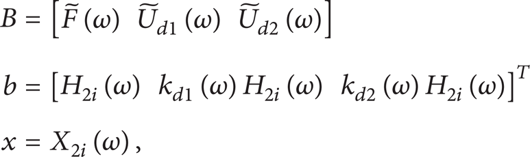
where B can be measured and the elements in b are unknown quantities needed to be identified; then (25) can be rewritten as

$Bb=x.$

(28)

Equation (28) can be regarded as a multivariate linear regression problem. The linear modal FRFs and nonlinear parameters can be estimated in a single step via least-squares method.

The NIFO method is modified to be applicable in continuous systems. The benefits of the modified NIFO method are obvious. (1) The method can be used in a continuous system with clearance nonlinearity. (2) By transforming the model from physical space to modal space, linear modal FRFs and nonlinear parameters can be identified at any order of natural frequency. (3) It makes no linearization assumption about nonlinear terms, so there is not any error caused by linear approximation in the identifying procedure. (4) The method can be applied to all kinds of nonlinear systems, even those containing more than one nonlinearity.

3.4. Simulation Results and Discussion

The transformation matrix should be firstly obtained before the RFS method and the NIFO method can be applied to the rigid-flexible coupled beam system with clearance. The transformation matrix converts the measured vibration response signal from physical space to modal space, which consists of the mode shape data at different measuring points.

The model is shown in Figure 9, and the parameters of this system are given in Table 2. In the controlled system the clearance plays the role of an external disturbance. As the controller has to work for every kind of contact, a very accurate estimation of c is not necessary [39]. So the damping coefficient c is also ignored.

Table 2:

Parameters of rigid-flexible coupled beam system with clearance.

l1 = l2 (m)	A1 = A2 (m2)	I1 = I2 (m4)	E (Pa)	ρ (kg/m3)	d1 = d2 (m)	k1 = k2 (N/m)
1	0.001	0.83e − 8	1.9e11	7850	0.005	1e6

As is discussed in Section 3.3, the oscillatory differential equations of the two beams are dispersed by employing the approach of assumed modes method. The first sixteen modes are hired to obtain the system's vibration response under the excitation of white noise. The displacement response in the middle and at the right end of the two beams is shown in Figures 12 and 13, respectively. It is obvious that the displacement response amplitude at the right end is larger than that in the middle, especially for beam 1 which is fixed at the left end. The beam 2 contains vibration type of rigid body: rigid motion and rigid rotation, which leads to the fact that the displacement response amplitude does not increase with x-coordinate. Through Figures 12 and 13, we can also conclude that the displacement response of beam 2 is sparser than that of beam 1, which is also caused by the existence of vibration type of rigid body.

Figure 12:

Displacement response in the middle of the two beams: (a) beam 1, (b) beam 2.

Figure 13:

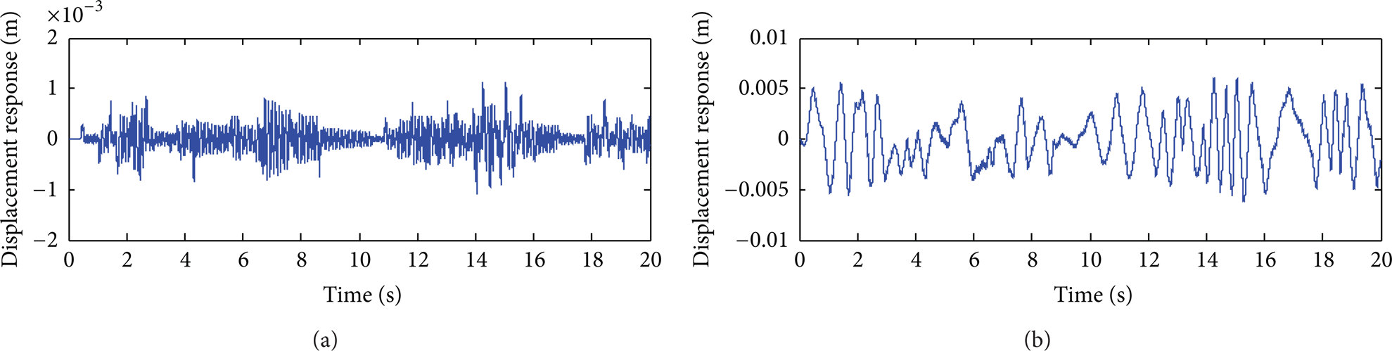
Displacement response at the right end of the two beams: (a) beam 1, (b) beam 2.

Figure 14 depicts the relative displacement at the contact point 1. The amplitude of the relative displacement is restricted between about −0.005 and 0.005. And the value above is the size of gap without question. In order to identify the system considered above, the RFS method should first be used to get clearance value. Under the third-order modal, the restoring-displacement curve (Figure 15) is plotted using calculated restoring force and relative displacement at contact point 1 (middle of the two beams). The clearance is identified as symmetrical with a value of 0.00502. This is because the occurrences of the displacement greater than 0.00502 decrease rapidly and the occurrences of the displacement less than 0.00502 remain about the same. It is the same case for the identification of −0.00502. It has to be mentioned that the identification error is 0.4%; this is acceptable. However the drawing result is not as good as Figure 7, which is mainly due to the following two reasons. (1) The restoring force contains two nonlinear forces and they cannot be separated in the restoring-displacement plot. (2) The restoring force contains linear forces which are caused by stiffness and damping which will make the curve deviate from ideal situation.

Figure 14:

Relative displacement at the contact point 1 (the middle of two beams): (a) contact point 1 (the middle of two beams), (b) enlarged drawing of (a).

Figure 15:

Identified clearance marked in the restoring-displacement curve.

The simulation was also implemented in the commercial software package MATLAB. The following parameters were used in the solution of (25): 40 averages, a Hanning Window, 50% overlap, and a block size of 25000. Amplitudes of the band limited Gaussian inputs were chosen to make nonlinear forces due to clearance at least about 15% of the total RMS value of the corresponding linear forces. It must be noted that the identification can be carried out when i is any value among 1, 2, 3, and 4. In the simulation, i was assigned 3 and the corresponding modal frequency was 53 Hz. The frequency range was chosen between 0 and 100 Hz.

The simulation results are displayed in Figure 16, which show the estimated value and estimated error of contact stiffness k₁ and contact stiffness k₂, respectively. It is obvious that the recognition precision is very low in the vicinity of the natural frequency. Although the maximum identification error reaches 60% and 100% for contact stiffness k₁ and contact stiffness k₂ at individual frequencies, respectively, the RMS error in 0–100 Hz is rather small: 0.115% and 2.65%. There are two main reasons for this phenomenon. One is that the frequency response function is very sensitive to leakage error in the vicinity of the peak. The other is that the correlation between the external exciting force and the two nonlinear forces increases significantly around the natural frequency.

Figure 16:

Estimation of contact stiffness k₁, contact stiffness k₂ and their identification errors: (a) k₁, (b) k₂.

Improving the frequency resolution is a common approach to solve the problem mentioned above. Figure 17 shows the estimation error of contact stiffness k₁ at different frequency resolutions. The maximum error of the identification decreases with the improvement of frequency resolution. Furthermore, the RMS errors listed in Table 3 decrease in order just like the maximum error.

Table 3:

RMS error at different frequency resolution.

Frequency resolution	RMS error of k1 (%)	RMS error of k2 (%)
0.005	0.181	2.68
0.0025	0.089	2.27
0.00125	0.043	2.11
0.000833	0.038	2.20

Figure 17:

Estimation error of contact stiffness k₁ and at different frequency resolutions: (a) 0.005, (b) 0.0025, (c) 0.00125, and (d) 0.000833.

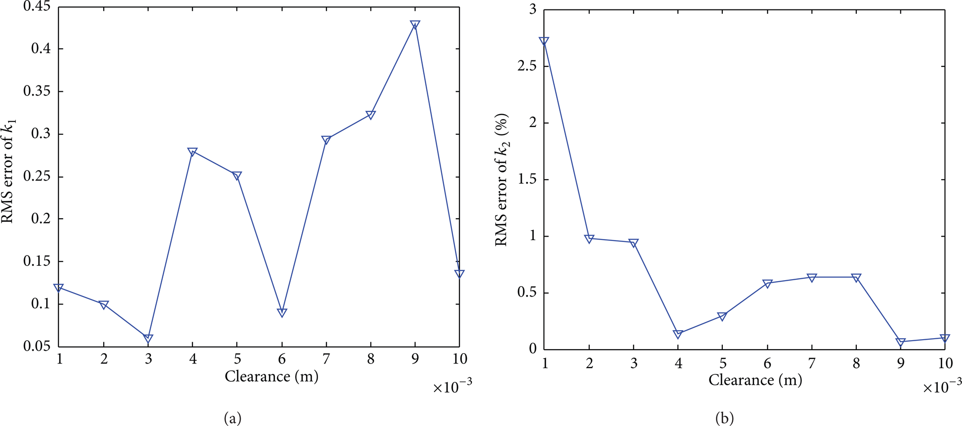
To study how contact stiffness affects the identification precision, the curves of the RMS error and contact stiffness are plotted in Figure 18 with our interested frequency range. The result shows that the RMS error is less than 2%, which indicates that the recognition precision is maintained at a very high level.

Figure 18:

RMS error at different contact stiffness: (a) contact stiffness k₁, (b) contact stiffness k₂.

A typical dynamical feature of the nonlinear response is the frequency-energy dependence of free oscillations [7]. In other words, the response of nonlinear system may be entirely different under different excitation energy. So it is essential to study the recognition error under different excitation energy. Figure 19 shows the curve of the RMS error and the exciting amplitude. It is plain that the error is fairly large when the excitation amplitude is small. But with the increase of the excitation amplitude, the recognition error first decreases and then increases. It must be noted that the change from being large to small or from being small to large is rather severe. The above characteristic can be explained as below. Under too small exciting force, the displacement response is so negligible that the clearance has no effect on the system. As a result, the response signal cannot reflect backlash nonlinear characteristic and the estimation is poor. When the excitation is big enough, the recognition precision grows significantly. However, if the excitation amplitude is too large, the characteristic signal caused by clearance will be submerged in the response signal. The identification effect will certainly be terrible.

Figure 19:

RMS error identified at different excitation amplitudes: (a) contact stiffness k₁, (b) contact stiffness k₂.

Clearance value is a prerequisite for the identification of contact stiffness by using NIFO method. Figure 20 depicts the curve of the clearance and the RMS error. It seems that the clearance value has little to do with the identification error under the same exciting force. Through the analysis above, there is an ideal range of the exciting force. If the change of the clearance does not affect the exciting force lying in the ideal range, then clearance value will not influence the identification. But if the change of the clearance makes the exciting force too small or big to the system, the clearance will surely affect the identification precision. In a word, the influence of the clearance depends on the amplitude of the exciting force.

Figure 20:

RMS error identified at different gaps: (a) contact stiffness k₁, (b) contact stiffness k₂.

4. Conclusions and Future Work

The paper focuses on the clearance identification and contact stiffness in the barrel-cradle structure of artillery system. Before carrying out the recognition process, the RFS method coupling the NIFO method was first applied to the SDOF system with clearance. The simulation results showed that the RFS method and NIFO method were effective to the system with clearance. Then a rigid-flexible coupled beam system with clearance was proposed to model the barrel-cradle structure. Then the two methods were modified to apply to the rigid-flexible coupled beam system with clearance. Based on the RFS method, clearance value was obtained by carefully analyzing the displacement response signal. The contact stiffness was identified by using NIFO method on the premise that clearance value was known. The relationship between the recognition precision and some physical quantities like clearance, contact stiffness, and amplitude of exciting force was also studied. The identification error in the vicinity of natural frequency decreases significantly with the improvement of the frequency resolution. In a word, the modified RFS and NIFO methods provide a good estimate of clearance and contact stiffness of the simplified barrel-cradle structure. Experiments on cannon clearance simulator will be carried out in the future work. It is not an easy work to conduct experiments associated with nonlinear, especially for those experiment devices which are close to the actual situation instead of being ideal. Even so it is expected that the developed method will be effective in the coming experiments and play a part in the engineering practice in the near future.

Conflict of Interests

The authors declare that there is no conflict of interests regarding the publication of this paper.