A lot of facts show that many researches just place emphasis on data aggregation or data fusion, which is not beneficial to analyze the sensed data thoroughly and will lead to the aggregation results' not being used fully; worse yet, the actual networks are always existed with lossy links; many now available aggregation algorithms are based on ideal network models and not any further analysis and fusion about aggregation results are done. Thus, we propose the concept of data fusaggregation so as to support processing sensed data while transmitting in large-scale probabilistic wireless sensor networks and propose a reliability-oriented data fusaggregation algorithm (RODFA) to assist users to get the monitoring information from the monitored geographic environment and measure the reliability of the information they get. RODFA also facilitates network administrator to improve the system sensing performance for large-scale probabilistic WSNs. In RODFA, the parameter η, which could reflect the reliability of aggregation result intuitively, is defined and calculated and it plays an important part in helping users to process aggregation result further. In our experiment, the validity of RODFA is verified by our simulation results, and the influence of network sizes and network performances on data fusaggregation is analyzed.
1. Introduction
Wireless sensor network (WSN) is a class of wireless ad hoc networks which consist of thousands of sensor nodes (SNs). Due to recent advance in microelectronics, wireless communications and sensor technologies have made the development of low-cost, low-power, multifunctional sensor nodes possible [1]. The capabilities of pervasive surveillance, sensor networks have attracted significant attention from many applications domains, such as habitat monitoring [2, 3], object tracking [4, 5], environment monitoring [6–8], military [9], traffic management [10], disaster management [11], and smart environments. In these applications, the aggregation and fusion of sensed data are very important for users to get the summary information from monitored areas. Many works about data aggregation and data fusion for WSNs emerged, which further promote the application domains of WSN [12–14]; however, firstly, the existing study rarely takes into consideration that SNs are restricted by resources due to low battery supply; secondly, most researches are aimed at studying the network capacity issue under ideal network model which does not match the actual network; thirdly, data aggregation and data fusion have different singular focus; for example, the focus of data aggregation is data transmitting while data fusion places emphasis on analyzing sensed data. Both data transmitting and analyzing are important to WSNs applications; lastly, there are few profound discussion and research on the network size's and network performance's influence on data fusaggregation result (which will be introduced in the next section). We will try to study these four issues in later sections.
Firstly, as energy resources provided for SNs are usually battery cells which are impossible to recharge during WSNs' working process, SNs are restricted by resources due to low battery supply. Consequently, in this paper, energy saving technology is taken into consideration, to make the network model more practical. For better energy utilization, we choose cluster-based WSNs [15, 16]. In cluster-based WSNs, SNs resident in nearby area would form a cluster and SNs can select one of the clusters to be their cluster-head nodes (CHs). The CH organizes data pieces received from SNs into an aggregated result and then forwards the result to the base station (sink node) along with the regular routing paths.
Secondly, to the best of our knowledge, lots of the studies mentioned above are based on ideal deterministic network model (DNM), where any pair of nodes in a network is either connected or disconnected. If two nodes are connected, that is, there is a deterministic link between them, and then a successful data transmission can be guaranteed as long as there is no collision. Otherwise, if two nodes are disconnected, the direct communication between them is assumed to be impossible. However, for real application, this DNM assumption is too ideal and not practical on account of the “transitional region phenomenon” [17, 18]. Because of the transitional region phenomenon, a large number of network links (probably more than 90%) become unreliable, which is named lossy links [17]. Even without collisions, data transmission over a lossy link is successfully conducted with a certain probability rather than being completely guaranteed. Therefore, a more practical network model for WSN is the probabilistic network model (PNM) [17], in which data communications over a link are successful with a certain probability rather than always being successful or always unsuccessful. For convenience, the WSNs considered under the DNM/PNM are called deterministic/probabilistic WSNs. Hence, in order to make our research much closer to the real network and get more practical value than existing studies, our research is under probabilistic WSN shown as the network model in Section 2.
Thirdly, in order to truly achieve processing sensed data while transmitting among network, users, and network administrator, we first present the concept of data fusaggregation which is based on the definitions of data aggregation and data fusion. In many applications, WSNs are mainly used for gathering data acquired from the physical environment to an external base station [19]. During a data gathering process, if the raw data can be aggregated and only an aggregation value is transmitted to the sink node, it is called data aggregation [20]. And data fusion is a widely adopted signal processing technique that can improve the system sensing performance by jointly considering the measurements of multiple sensors [21]. As data aggregation and data fusion are both playing important functions in many applications of WSNs and they have different focuses, the realization of processing sensed data while transmitting has started to become important for WSNs. Thus, data fusaggregation is presented in our research as follows.
Definition 1 (data fusaggregation).
The raw data can be aggregated; only one aggregation value will be transmitted to the sink node. And through analyzing the aggregation value, the sink node will get some other information which could measure the performance of network or be useful to users.
Lastly, on the basis of the concept of data fusaggregation, a data fusaggregation algorithm is proposed to comprehensively analyze and use sensed data to facilitate the improvement of system sensing performance. This algorithm is named reliability-oriented data fusaggregation algorithm (RODFA). In this algorithm, firstly, the parameter η (the lower limit value of reliability) is defined to measure the reliability of aggregation result. Then we obtain the formula for calculating the value of η through theoretical derivation. Lastly, the aggregation result and the parameter η will be sent to users through the sink which could be a reference for users' handling the information they get. In our experiment part, we first study the influence of network size and network performance on RODFA result.
The rest of this paper is organized as follows. In Section 2, the network model is discussed; it includes the assumptions of this model and the problem definitions. In Section 3, we describe the mathematic foundations of RODFA. The calculation of η for one is given in Section 4. Section 5 shows the validity of RODFA. And we discuss factors affecting the RODFA (network size and network performance) in Section 6. In the last section, we conclude the paper.
2. Network Model
2.1. Assumptions of the Model
In this paper, we consider that a large-scale probabilistic WSN consists of N sensors. Let be the number of active SNs in the monitored area at time t. is varying with time and unknown by the sink. Let be the sensed data of active sensor node i at time t, and let be the set of all the sensed data in monitored area at time t. is stored in the active sensor node i for . Since all sensed data are bounded, we use to denote the upper bound of all sensed data.
On the basis of the analysis in Section 1, for better energy utilization, we apply the dynamic minimal spanning tree routing protocol (DMSTRP) to our network model and our radio power model is similar to [22]. The DMSTRP is a cluster-based routing protocol for large-scale wireless sensor networks which is proposed in [23]. According to [23], in our network model, the monitored geographical area is divided into a number of clusters which are formed similar to [24], and the clusters are disjoined with each other. Here, assume that the monitored geographical area is fully covered by active sensors, and it is divided into n clusters. Let ω be the maximum of network's layers at time t, and let be the numbers of nodes in the , at time t, respectively. Let be the set of all sensed data in layer 1 at time t, and let be the set of all sensed data in at time t, respectively.
When the sink node initiates one time of data collection at time t, we let d be the distance of all lossy links, the lossy links are successfully conducted with a certain probability q, and let be the set of all sensed data which are sensed successfully to sink from layer 1 at time t. Thus, the sensed data of layer 2, layer 3,…, layer ω will be sent successfully to the sink with a certain probability , respectively, and let be the set of all sensed data which are sensed successfully to sink node from the at time t, respectively. And the function relationship between q and d will be presented in the next section.
2.2. Problem Definition
In this paper, when researching on data fusaggregation, we take SUM operation, for example, and propose RODFA to comprehensively analyze and use sensed data for facilitating further promotion of WSNs' application domains. The exact sum of the monitored area at time t is defined as . We will briefly introduce some related definitions of reliability as follows before introducing the steps of RODFA.
Definition 2 (ε-estimate).
is called as an ε-estimate of if for any ε ().
Definition 3 (reliability).
For a given network and ε (), reliability is the probability of whether is the ε-estimate of .
Definition 4 (η).
For a given network and ε (), η () is the lower limit value of probability of whether is the ε-estimate of ; that is, and we call it the lower limit value of reliability.
η is an important parameter which could measure the reliability of aggregation results. It will be sent to users for facilitating the next handling of aggregation result, should the users regard the aggregation result as a decision-making or just a reference point, even discard this aggregation result directly. The calculation of η will be completed in RODFA. The main steps of RODFA are shown as Figure 1, and they can be described as follows in detail.
The main steps of RODFA.
Step 1.
Sink node launches one time of data collection and sends the data acquisition command to every cluster, and the clusters will retransmit this command to their own child nodes.
Step 2.
According to [22], every node will send its sensed data to its cluster node. And after analyzing and processing the sensed data, the cluster will retransmit the processing result to sink node.
Step 3.
Sink node will get an approximate sum which will be discussed in Section 3: .
Step 4.
According to the formula of η (where , and the derivation process of this formula will be given in Section 4), sink node will calculate the value of η and turn it back to users with together, or turn it back to the network administrator for facilitating the administrator to improve the system sensing performance. And the algorithm stops.
Combined with the above steps of RODFA, the key of RODFA is to obtain the value of η of . And the problem of computing the value of η is defined as follows.
Input:
, ;
ε (), ω, and q;
aggregation operator sum.
Output:
The value of η of the mathematic estimator of sum: .
For facilitating the later analysis, we will give the other two definitions of unbiased estimate and delay.
Definition 5 (unbiased estimate).
is an unbiased estimate of if the mathematical expectation of is equal to , that is, ; otherwise is a biased estimator of .
Combining [23], DMSTRP connects nodes in clusters by MSTs. In each cluster, all nodes including the CH are connected by a MST and then the CH as a leader to collect data from the whole tree. All CHs are connected by another MST to route toward sink. And the processing of data fusing is handled along with the tree route. The average transmission distance of each node can be reduced by using MSTs as Figure 2 shows, and thus the energy dissipation of transmitting data is reduced.
A MST in DMSTRP.
In Figure 2, node 1, node 2, and node 6 are leaf nodes; node 3 and node 5 are father nodes; node 4 is the cluster head node. Because node 1 and node 2 have the same father, only node 1 can transmit in the first period. Thus the first period transmitting queue is ; this means node 1 and node 6 can transmit their data at the same time. We can get the transmitting queue in the following period as and . Based on the above analysis, we define delay as follows.
Definition 6 (delay).
The amount of periods from the sink node initiates a data collection command to all sensed data from SNs being sent to the sink node, no matter how long it will last. This amount of time is called one delay.
According to the concept of delay, we can get that the delay of Figure 2 is Figure 3.
Verifying the validity of RODFA for network with 5000 m × 5000 m size, and for the red forked line, as when all relevant information in the network is fixed and immovable, the values of q and ω are constant, and the value of η of will show a trend of increase with the increase of the relative error bound ε. Thus, we just describe the calculation results for η on a scale of 0 to 1; that is .
3. Mathematic Foundations
The calculation of probability q is the foundation of RODFA. Existing studies show that the probability q will be a function of distance d (the distance between any pair of nodes is connected). Next, we will briefly describe the derivation of this function and then do research on the estimator of sum.
3.1. Relationship between q and Distance d
Let r be the receiving signal-to-noise ratio (SNR) and let f be the length of one frame, and then the functional relationship between q and r can be described as [18]
In this paper, the propagation model is lognormal shadowing model [25], and the relationship between r and the distance d will be obtained in next section.
Let be the path loss for one certain location, the reference distance, β the path loss exponent, and Gaussian random variable available for zero mean. Then the relationship between and d can be described by formula (2) and in units of dBm:
On the basis of formula (2), we assume that is the output power of the sender and is the power that the receiver received. Then can be obtained from the following:
Let be the platform noise and combined with the relationship (3) between the SNR and the power received by the receiver; we can see that
Once the model is determined, all of the parameters in the above formulas will be only given. As we set the propagation model to be lognormal shadowing model, the parameter settings for our experiment are similar to [26]. Combined with the above formulas (1)–(4), we can obtain the relationship between q and d that can be shown as
3.2. Estimator of Sum
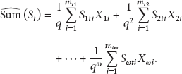
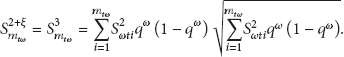
Let be the sets of sensed data in layer 1, layer 2, layer 3, …, layer ω at time t, respectively, and let be the sets of all sensed data which are sensed successfully to sink node from the layer 1, layer 2, layer 3, …, layer ω at time t, respectively. The mathematic estimator of sum is denoted by , and the can be computed by
where q is the probability in which lossy links are successfully conducted at time t. And according to the above definition of the unbiased estimate, Theorem 7 shows that is the unbiased estimator of the exact sum .
Theorem 7.
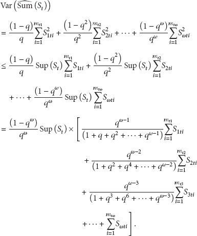
Let be the mathematical expectation of and let be the variance. Then,
Proof.
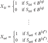
For any , set random variables satisfy the following equations, respectively:
Clearly, there are , , , ,…, , and . Meanwhile, according to the lognormal shadowing model, for , there exist the random variables and that are independent of each other (). Furthermore, according to the distribution of , there are , , , .
Theorem 7 shows that the mathematic estimator of sum is the unbiased estimator of the exact sum . The upper limit of the variance value is inversely proportional to the probability q. That is to say, with the probability q increasing, the upper limit of can be arbitrarily small. Thus, referring to [27], with the increase of q, the relative error between and will gradually decrease, and if q is sufficiently large, this relative error can be arbitrarily small.
4. Calculating η of
According to the steps of RODFA in Section 2.2, the key step is to calculate η of . Thus, we will research on this issue next.
The steps of calculating the value of η are (1) proofing that obeys the normal distribution; (2) transforming the normal distribution into standard normal distribution; and (3) utilizing the characteristics of standard normal distribution to calculate the value of η.
For any i, let the variable () be as follows:
There is . Firstly, we need to proof that obeys normal distribution. In view of the linear combination of n independent normal distribution functions still obey normal distribution through proofing that the sum of each layer data obeys normal distribution to proof that obeys the normal distribution. Reference [28] shows that, if each layer data conforms to Lyapunov condition, the sum of each layer data will be in accordance with the application conditions of the central limit theorem; that is, the sum of each layer data will obey the normal distribution. And Theorem 8 proofs that the data in layer 1, layer 2, …, layer ω conform to Lyapunov condition, respectively.
Theorem 8.
The ω groups of sequence of random variables () satisfy the Lyapunov condition; that is satisfy the following formula:
Among them, , is the number of data in layer k at time t, , and for , there are and .
Proof.
Combining Section 2, the sensed data of the layer 1, layer 2, layer 3,…, layer ω will be sent successfully to the sink with a certain probability , respectively. are the set of all sensed data in layer 1, layer 2, layer 3, …, layer ω at time t, respectively, and are the sets of all sensed data which are sent successfully to sink node from layer 1, layer 2, layer 3, …, layer ω at time t, respectively.
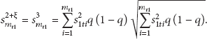
For Layer 1 . There is , and .
Order , according to the above analysis, for , there is
Among them, and , respectively, present the lower limit and upper limit of sensed data in layer 1. , ; hence . Meanwhile, and ; therefore . In conclusion, ; that is, when , there is to satisfy formula (14) in Theorem 8, and satisfies the Lyapunov condition. According to [28], meets the application conditions of central limit theorem; that is, obeys normal distribution.
Omitting the analysis of other layers (the researching method for other layers is same as ), we will then describe the analysis of layer ω; that is, .
For Layerω. Same as the analysis of , when , there are and . For , if we let , then there will be
Combining formula (18) with formula (19), there is
That is, for layer ω, satisfies the formula (14) in Theorem 8 to make , and also satisfies the Lyapunov condition. According to [28], meets the application conditions of central limit theorem; that is, obeys the normal distribution.
Theorem 8 shows that the ω groups of random variable sequences () satisfy the Lyapunov condition. That is, the sum of each layer data obeys normal distribution. As whether the sensed data in each layer can be sent successfully to sink node is independent of each other, so is the sum of these ω independent variable normal distributions . Thus obeys normal distribution. For a given relative error limit ε, Theorem 9 describes the calculation of η of .
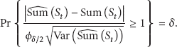
Theorem 9.
Supposing , is the quantile of standardized normal distribution, if satisfies the following formula:
Then, the probability that the relative error between and satisfies the given error limit ε will be equal or greater than η; that is,
Proof.
From formula (21), there is . As and are, respectively, the lower limit of and the lower limit of the value of all sensed data, so there is . Hence,
Theorem 7 shows that , , and as obeys normal distribution, from formula (23), there is
Combining the knowledge of standard normal distribution quantile [29], (23), (24), and , there is
5. Validity of RODFA
To evaluate RODFA, we use Matlab to simulate a sensor network of 5000 nodes. Using the above 5000 nodes and 285 cluster-heads randomly deployed in network area of 5000 m × 5000 m, 10000 m × 10000 m, 15000 m × 15000 m, we make the DMSTRP protocol running in the simulation network system to connect all nodes and cluster-heads into a whole. For time t in ready phase, we can obtain the maximum of network's layers ω through counting the numbers of layers of all clusters. As all the nodes are randomly deployed in network area, and as far as possible to ensure uniformity in the process of deploying, we can randomly select one cluster from the network, and then to obtain the distance d of all lossy links through calculating the mean distance of all distances between every two linked nodes in this cluster. Plugging this distance d into formula (5), then we can get the probability q at time t.
This group experiments are to investigate whether RODFA is valid. As data communications over a link is successful with a certain probability rather than always being successful or always fail in probabilistic WSNs [17], every time we calculate the reliability of , we will get the different reliability value even if all relevant information of the network is fixed and immovable (i.e., the number of active nodes, the structure of the cluster, the number of clusters, the number of nodes in every cluster, the distance of all links, and the layout of all nodes are changeless).
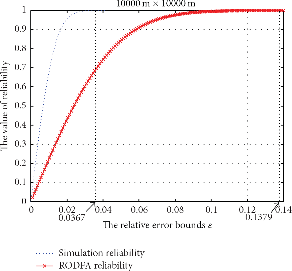
We do 10000 times of calculations when all relevant information in the network is fixed and immovable and let the initial energy of sink node, cluster-heads, and nodes be large enough (no node will die in experiment process). For these 10000 calculations, we calculate the relative error between and ( and obtained from our simulation network. In order to get the value of , in this experiment, we assume that the CHs will not only retransmit the aggregation result to sink node but also relay all sensed data that are from other SNs or CHs and then do statistics analysis on cumulative probability under different relative error bounds ε, shown as the blue dashed lines in Figures 3, 4, and 5, and we call this reliability as statistical reliability. Furthermore, according to the above analysis, sink node can get the values of ω and q for time t easily, and after putting ω and q in , we can calculate the value of η of for every relative error bound ε and then describe the line of η as the red forked lines in Figures 3, 4, and 5, and we call this reliability as RODFA reliability.
Verifying the validity of RODFA for the network with 10000 m × 10000 m size and we only describe the calculation results for ε on a scale of 0 to 0.14 in the red forked line.
Verifying the validity of RODFA for the network with 15000 m × 15000 m size, where we only describe the calculation results for ε on a scale of 0 to 0.18 in the red forked line.
Figures 3, 4, and 5, respectively, illustrate the statistical results from simulation experiments (statistical reliability) and the calculation results from RODFA (RODFA reliability) for network area of 5000 m × 5000 m, 10000 m × 10000 m, 15000 m × 15000 m. In Figure 3, the blue dashed line shows that the statistical reliability for ε = 0.0225 is 0.9999, and the red forked line shows that, when the RODFA reliability η of reaches 0.9999, the relative error bound ε between and will be 0.0907, and the difference between 0.0225 and 0.0907 is 0.0682. Furthermore, the blue dashed line also demonstrates that, for the network with 5000 m × 5000 m size, the maximum of the relative error bound ε between and from the network simulation results is 0.0234. In Figure 4, it can be found that when the statistical reliability of (shown as the blue dashed line) reaches 0.9999, ε is equal to 0.0367; and the calculation results of RODFA demonstrate that, when RODFA reliability η reaches 0.9999, the relative error bound ε will be 0.1379, and the difference between 0.0367 and 0.1379 is 0.1012. In addition, the blue dashed line also shows that the maximum of the relative error bound ε between and from the network simulation results is 0.0413. In Figure 5, when the statistical reliability of reaches 0.9999, the relative error bound ε is equal to 0.0508; and the red forked line shows that, when RODFA reliability η of reaches 0.9999, the relative error bound ε will be 0.1768, and the difference between 0.0508 and 0.1768 is 0.126. Furthermore, the blue dashed line also demonstrates that the maximum of the relative error bound ε in the network simulation results is 0.0513.
After describing the comparative analysis of each figure separately, we will investigate and analyze the relevant feature details shown in Figures 3, 4, and 5 later.
Firstly, the three figures show that the maximums of relative error bounds ε for blue dashed lines are all small. These numbers show that the data aggregation method in our paper has better approximating effect, and it is also corresponding to the proof that is an unbiased estimate of . Secondly, there is a gap between blue dashed line and red forked line in each figure, and reasons for this phenomenon are as follows: (1) the zooming out in the formula derivation process of upper limit variance of ; (2) just considering the distance d and neglecting other factors which also affect the value of q between two connected nodes. (3) In these three figures, due to the increase of network area, the statistical reliabilities go down (for a same relative error value) and the maximums of relative error bounds ε between and grow bigger (from 0.0234 to 0.0513, shown as the blue dashed lines in these three figures). (4) With the increase of network area, the RODFA reliability η is falling, but its changing rate is greater than that of the statistical reliability ().
The above analysis indicates that the RODFA is validity, and η of which is calculated by RODFA has a greater likelihood to be the minimum of reliability.
6. Discussing the Factors Affecting RODFA
The aim of the former part of the experiment is to demonstrate the effectiveness of RODFA. Next we will turn RODFA embedded in our simulation network and investigate the factors affecting RODFA. We use Matlab simulator to implement a wireless sensor network. To ensure that the simulation results in this paper are correct, we use our simulator to do the same experiments (the network lifetime) of DMSTRP that use C/C++ in [23] and get the approximately same results. And the optimal number of clusters in our simulative network is adopted according to [30].
In this section, the first group of experiments is to describe the changing trend of the value of η of (calculated by RODFA) with the increase of network running rounds. And the experiment results for different network areas are shown in Figure 6.
η of in network area of 5000 m × 5000 m (blue), 10000 m × 10000 m (red), and 15000 m × 15000 m (green). From the blue line, we can find that the value of η is 0 from the 0th to the 9th round, and in the 9th round, the value of η leaps to 0.9611 and lasts for 400 rounds. In the 409th round, the value of η suddenly reduces to 0.9457 and lasts for 210 rounds, and then there has a sudden drop of η in the 619th round. Then η has a sustained downward trend until its value becomes 0. The red line shows the η of in network area of 10000 m × 10000 m. We can find that, among the first 11 rounds, the value of η is 0, and then it leaps to 0.9133 in the 11th round and lasts for 300 rounds. In the next 200 rounds (from the 311th round to the 511th round), η is 0.8742, and in the 511th round, the value of η reduces to 0.8504 again. After a sudden drop in the 631th round, η has a sustained downward trend until its value becomes 0. The green line describes the η of in network area of 15000 m × 15000 m. η = 0 for the first 13 rounds, and in the 413th round, η has a sudden drop, and then its value continues to fall until it becomes 0.
Due to these three lines belonging to the same type of experimental result, we will just analyze the blue curve shape in Figure 6. The blue line describes the changing trend of η with the increase of network running rounds for network of 5000 m × 5000 m (when ). As the establishment of clusters will take a certain amount of time (how long does it take is based on network area and active nodes number), that is why η is 0 from the 0th round to the 9th round. After the sink node obtaining the values of q and ω (ω = 3 and q = 0.9308), RODFA will work out the value of η and η leaps to 0.9611 in the 9th round.
Based on the above analyses, the values of q and ω mainly depend on network area, active nodes number, and internal structure of cluster and so on. As all of these three lines are describing the simulation results of network with certain area, thus we do not need to investigate the inference of network area on q and ω. From the blue line, we can find that the number of active nodes is 5000 in the first 610 rounds. But near the 400th round, clusters are remodeled, which makes the network structure changed; it also changes the values of q and ω. Thus, following the 409th round, η suddenly reduces to 0.9457 and lasts for 210 rounds. Secondly, the active nodes number begins to decline from the 600th round. As setup phase and ready phase continuously cycle in the network, the values of q and ω are different for different time. That leads to the result that η has a sustained downward trend until its value becomes 0 from the 619th round. Lastly, we also find that η is lower in the subsequent 123 rounds (from the 811th round to the 934th round). That is because the active nodes number remains at a low level in the subsequent rounds of network running, while less active nodes deploy in the network with a certain area, the value of ω will be larger and q will be smaller, which makes η small.
The second group of experiments is to investigate the influence of network size on RODFA. According to , the value of η required given ε, q, and ω. Based on the above analysis, the values of q and ω depend on network size when the routing protocol is certain. And as the value of ε is given by user's application requirement, η will change with the difference of network area. As shown in Figure 7, when ε is, respectively, set to be 0.01, 0.03, and 0.05, η decreases with the growth of network size.
The influence of network size on RODFA, where ε, respectively, is set to be 0.01, 0.03, and 0.05. The number of nodes is 5000. The values of η for these three ε are calculated while the network size increases from 5,000 to 15,000.
The last group of experiments is to analyze the network delay. According to the definition of delay in Section 2, we can get the delays of simulation network models with size of 5000 m × 5000 m, 10000 m × 10000 m, and 15000 m × 15000 m and describe them in Figure 8. Figure 8 shows that the network delay fluctuates up and down in 524 when the number of alive nodes is more than 1500; while when the number of alive nodes is less than 1500, the value of network delay begins to decrease until its value becomes 0. Probably this is due to the numbers of links and clusters in the network, and the value of network ω decreases with the decrease of alive nodes in the network, which lead to the changing trend of network delay shown in Figure 8.
The delay of network under different size.
7. Conclusions
Our proposed algorithm, RODFA, belongs to a data fusaggregation algorithm which mainly includes aggregating sensed data from large-scale wireless sensor networks and doing fusion analysis of the aggregation results. We choose SUM to design RODFA in this paper and the main idea of RODFA is to calculate the parameter η of through auto analysis and synthesizing of . It can provide η to users and facilitate them to do the next handling of ; also it can facilitate the network administrator to improve system sensing performance. Experiments in Section 5 indicate that the parameter η, which is calculated by RODFA, has a greater likelihood to be the minimum of reliability and RODFA is valid. In Section 6, we first investigate the influences of network size and network performanceon data fusaggregation to guide the network administrator on improving the system sensing performance.
Footnotes
Conflict of Interests
The authors declare that there is no conflict of interests regarding the publication of this paper.
Acknowledgment
The project is supported by The National Key Technology Research and Development Program of the Ministry of Science and Technology of China (Grant no. 2012BAH82F04).
References
1.
HuangG.ZomayaA. Y.DelicatoF. C.PiresP. F.Long term and large scale time synchronization in wireless sensor networksComputer Communications201437779110.1016/j.comcom.2013.10.003
2.
RozyyevA.HasbullahH.SubhanF.Indoor child tracking in wireless sensor network using fuzzy logic techniqueResearch Journal of Information Technology20113281922-s2.0-8005478715110.3923/rjit.2011.81.92
3.
SzewczykR.OsterweilE.PolastreJ.HamiltonM.MainwaringA.EstrinD.Habitat monitoring with sensor networksCommunications of the ACM200447634402-s2.0-424311408710.1145/990680.990704
4.
WangZ. B.LouW.WangZ.MaJ. C.ChenH. L.A hybrid cluster-based target tracking protocol for wireless sensor networksInternational Journal of Distributed Sensor Networks201320131649486310.1155/2013/494863
5.
GarciaO.QuinteroA.PierreS.A global profile-based algorithm for energy minimization in object tracking sensor networksComputer Communications20103367367442-s2.0-7604909061910.1016/j.comcom.2009.11.020
6.
ZhangJ.SongG. M.QiaoG. F.LiZ.WangA. M.A wireless sensor network system with a jumping node for unfriendly environmentsInternational Journal of Distributed Sensor Networks20122012856824010.1155/2012/568240
7.
SabriN.AljunidS. A.AhmadB.YahyaA.KamaruddinR.SalimM. S.Wireless sensor actor network based on fuzzy inference system for greenhouse climate controlJournal of Applied Sciences20111117310431162-s2.0-8005284495010.3923/jas.2011.3104.3116
8.
KumarD.Monitoring forest cover changes using remote sensing and GIS: a global prospectiveResearch Journal of Environmental Sciences2011510512310.3923/rjes.2011.105.123
9.
BekmezciI.AlagözF.Delay sensitive, energy efficient and fault tolerant distributed slot assignment algorithm for wireless sensor networks under convergecast data trafficInternational Journal of Distributed Sensor Networks2009555575752-s2.0-7044962515110.1080/15501320802300123
10.
ChenY. L.LaiH. P.A fuzzy logical controller for traffic load parameter with priority-based rate in wireless multimedia sensor networksApplied Soft Computing20141459460210.1016/j.asoc.2013.08.001
11.
TsengY.-C.PanM.-S.TsaiY.-Y.Wireless sensor networks for emergency navigationComputer200639755622-s2.0-3374636913910.1109/MC.2006.248
12.
DeligiannakisA.KotidisY.RoussopoulosN.Processing approximate aggregate queries in wireless sensor networksInformation Systems20063187707922-s2.0-3374870425010.1016/j.is.2005.02.001
13.
FanY.-C.ChenA. L. P.Efficient and robust sensor data aggregation using linear counting sketchesProceedings of the 22nd IEEE International Parallel and Distributed Processing Symposium (IPDPS '08)April 20081122-s2.0-5104910574810.1109/IPDPS.2008.4536265
14.
TanR.XingG. L.YuanZ. H.LiuX.YaoJ. G.System-level calibration for data fusion in wireless sensor networksACM Transactions on Sensor Networks20132893128
15.
EliasJ.Optimal design of energy-efficient and cost-effective wireless body area networksAd Hoc Networks201413, part B56057410.1016/j.adhoc.2013.10.010
16.
ChenY.-L.LinJ.-S.Energy efficiency analysis of a chain-based scheme via intra-grid for wireless sensor networksComputer Communications20123545075162-s2.0-8485641501910.1016/j.comcom.2011.12.002
17.
LiuY.ZhangQ.NiL.Opportunity-based topology control in wireless sensor networksIEEE Transactions on Parallel and Distributed Systems20102134054162-s2.0-7674915497210.1109/TPDS.2009.57
18.
ZunigaM.KrishnamachariB.Analyzing the transitional region in low power wireless linksProceedings of the 1st Annual IEEE Communications Society Conference on Sensor and Ad Hoc Communications and Networks (IEEE SECON '04)October 20045175262-s2.0-20344378689
19.
WangT. C.QinX. L.LiuL.An energy-efficient and scalable secure data aggregation for wireless sensor networksInternational Journal of Distributed Sensor Networks201320131184348510.1155/2013/843485
20.
WanP.-J.HuangS. C.-H.WangL.WanZ.JiaX.Minimum-latency aggregation scheduling in multihop wireless networksProceedings of the 10th ACM International Symposium on Mobile Ad Hoc Networking and Computing (MobiHoc '09)May 20091851942-s2.0-7045017743110.1145/1530748.1530773
21.
VarshneyP. K.Distributed Detection and Data Fusion1996Springer
22.
HeinzelmanW. R.ChandrakasanA.BalakrishnanH.Energy-efficient communication protocol for wireless microsensor networksProceedings of the 33rd Annual Hawaii International Conference on System SiencesJanuary 20002232-s2.0-0033877788
23.
GuangyanH.XiaoweiL.JingH.Dynamic minimal spanning tree routing protocol for large wireless sensor networksProceedings of the 1st IEEE Conference on Industrial Electronics and Applications (ICIEA '06)May 2006Singapore152-s2.0-4274909967110.1109/ICIEA.2006.257220
24.
MuruganathanS. D.MaD. C. F.BhasinR. I.FapojuwoA. O.A centralized energy-efficient routing protocol for wireless sensor networksIEEE Communications Magazine2005433S8S132-s2.0-1774437620010.1109/MCOM.2005.1404592
25.
FazioP.de RangoF.SottileC.A new interference aware on demand routing protocol for vehicular networksProceedings of the International Symposium on Performance Evaluation of Computer and Telecommunication Systems (SPECTS '11)June 2011981032-s2.0-80052645976
26.
HeS. M.Research on the Key Technology of Opportunistic Routing in Multi-Radio Multi-Channel Wireless Mesh Network2013Hunan, ChinaHunan University
27.
BernsteinS.BernsteinR.Elements of Statistics Ii: Inferential Statistics20041stColumbus, Ohio, USAMcGraw-Hill
28.
FischerH.A History of the Central Limit Theorem: From Classical to Modern Probability Theorem20111stNew York, NY, USASpringer
29.
ShenZ.XieS. Q.PanC. Y.Probability Theory & Mathematical Statistics2005Beijing, ChinaHigher Education Press
30.
LindseyS.RaghavendraC.SivalingamK. M.Data gathering algorithms in sensor networks using energy metricsIEEE Transactions on Parallel and Distributed Systems20021399249352-s2.0-003676661610.1109/TPDS.2002.1036066