Motion of Passive Scalar by Elasticity-Induced Instability in Curved Microchannel

Abstract

This paper presented a direct numerical simulation (DNS) study on the elasticity-induced irregular flow, passive mixing, and scalar evolution in the curvilinear microchannel. The mixing enhancement was achieved at vanishingly low-Reynolds-number chaotic flow raised by elastic instabilities. Along with the mixing process, the passive scalar transportation carried by the flow was greatly affected by the flow structure and the underlying interaction between microstructures of viscoelastic fluid and flow structure itself. The simulations are conducted for a wide range of viscoelasticity. As the elastic effect exceeds the critical value, the flow tends to a chaotic state, while the evolution of scalar gets strong and fast, showing excellent agreement with experimental results. For the temporal changing of scalar gradients, they vary rapidly in the form of isosurfaces, with the shape of “rolls” in the bulk and evolving into “threads” near the wall. That indicates that the flow fields should be related to the deformation of viscoelastic micromolecules. The probability distribution function analysis between micromolecular deformation and flow field deformation shows that the main direction of molecular stretching is perpendicular to the main direction of flow field deformation. It implies they are weakly correlated, due to the confinement of channel wall.

1. Introduction

Chaotic flow occurs for the viscoelastic fluids at very low Reynolds number (Re). Since the inertial effect is trivial, such kind of flow state is called purely elastic instability or elastic turbulence which have been identified in a vast range of macroscopic and microscopic flow geometries with curvilinear streamlines, such as Taylor-Couette device, parallel-disk, cone-and-disk, and serpentine microchannels [1–3]. The viscoelastic fluids are typically the solutions of polymers or surfactants, and they have analogous flexible microstructures which deform with the flow. Considering the nature of elastic effect of viscoelastic fluid in different flows, these instabilities are driven by large positive primary normal stress difference N₁ and suppressed by negative second normal stress difference N₂. On the balance of fluid nature and the flow geometries, the elegant Pakdel-McKinley condition unifies the critical threshold for the onset of elastic instabilities [4]. Combination between fluid elasticity and curvatures of device is concluded to be the premise to excite the purely elastic instabilities or elastic turbulence. Without the confinement of curved walls, instabilities can hardly happen for very-low-Reynolds-number flow if no external perturbation is imposed. It is worth noting that the slow three-dimensional recirculation flow of shear-banded fluids in the straight microchannel is due to the interfacially driven undulation caused by the jump in second normal stress across the interface [5, 6]. And if the disturbance is not sufficiently large, the disturbance itself will damp by viscous forces [7]. As the elastic instability grows, the purely elasticity-driven turbulence hereby emerges. Also, recently there are numerical and experimental evidence of that the nonlinear elastic instability and even elastic turbulence could be generated in the straight microchannels [7, 8]. Note that their irregular flow state should be sustained by the outside perturbation, for instance, like numerically introducing a sinusoidal force term into the momentum equation and also constitutive equation or placing a variable number of obstacles in the center microchannel. In contrast, those perturbations are not necessary for curved geometries since they could maintain the nonlinearity by themselves. For the excitation and persistence of elastic turbulence in curved geometries, their functioning mechanism is suggested to be similar to “dynamo effect” [9]. The perturbation imposed in the flow induces the additional wavy deformation on the curved streamlines which associate the flexible long-chain molecular structures. And in turn, such deformations in the long-chain molecules raise local variation of stresses to the flow field as feedback. Thus, perturbation reveals itself in a positive way with the viscoelastic fluid flow, and the flow accelerates the perturbation via the flexible molecular motion. As such nonlinearity of elastic effect increases, the flow is proven to be chaotic, which resembles the developed turbulence condition in the statistic characteristics [3, 4]. However, it behaves stochastic in time, but smooth in space, which differs from the hydrodynamic turbulence.

As aforementioned, the elastic instabilities and turbulence stem from the peculiar fluid structures and their motion, which lead to the fast energy transportation. Therefore, as to the passive particles carried by those elasticity-induced irregular flows, they could be transported much forcefully than that in Newtonian fluids cases. Newtonian fluids are known to completely remain laminar flow at very-low Reynolds. So the elastic turbulence is promising for the mixing process and reagents reaction in the microfluidic applications, besides of the electrokinetic effect, electrophoresis, acoustic stream, magnetic driving and other active methods [10–12] to promote mixing. It could be widely employed for most of microfluidic manipulation circumstances, as a passive way of mixing. In this regard, it is probably the optimal option for microfluidic field where needs to mix fluids by the flow itself.

Chaotic mixing by viscoelastic fluid flow in the microfluidic devices has been intensively investigated, with a wide variety of layouts of microchannels [4, 11, 13]. And by the curved microchannel, efficient mixing enhancement has been achieved due to the chaotic flow. Whilst the mixing effect by elastic turbulence has been studied a lot in aspects of mixing length, mixing time, and scalar statistic moment, studies of scalar evolution and motion with time during the mixing process have been much scarcer, especially in the confined microchannels. Ottino and Wiggins proposed that the key factor to mixing enhancement lies in the effectiveness of the magnitude of cross-sectional flow, that is, to create as many contact interfaces as possible between two fluids in the cross-section of the flow direction [14]. The stretching and folding of the interfaces indicate that the flow structure forms Swiss-roll-like shape, which could be accomplished with the flexibility and elasticity of viscoelastic fluids in the motion. Along with the rolling process, the flow-carried scalars are thus transferred by this kind of “forced” chaotic convection, and their evolution is in a ramp-cliff variation temporally and spatially [15, 16]. As for a developed inertial turbulence, the scalar evolution has been studied in a three-dimensional straight channel flow, and it is found that the scalar dissipation shows a thin-layer structure, which is strongly related to the orientation of scalar gradient [17]. Considering the disparities of how the turbulence flow is driven, the scalar evolution should be accordingly behaving unusual in an elasticity-induced irregular flow. And that should be bound up with the motion and deformation of internal microstructures of working fluids.

For scalar transportation in the viscoelastic fluids flow in the curvilinear microchannel, so far there is no information of scalar gradient evolution and its relationship to fluid nature have been reported, to our knowledge. The present authors are of the opinion that a detailed perspective of scalar transportation for a three-dimensional chaotic viscoelastic flow has not been reached yet. The previous work by coauthors [18] has already made a comprehensive analysis on the vortex structures, scalar transportation by elastic instability in the curved channel. The present work further attempts to get a deep understanding on the scalar transportation evolution and its mechanism. The objective of this paper is to investigate the passive particles (scalar) transportation carried by the irregular viscoelastic fluids flow, combining the numerical simulations with the former experimental results. By direct numerical simulation (DNS) conducted in a curved microchannel unit geometry, the relationship between flow structures and the deformation of flexible molecules is elucidated. Also the mixing effect and mixing efficiency with elasticity variation are displayed, and the comparison with the experiments makes the mixing enhancement straightforward. Furthermore, simulations on various flow conditions would clarify our understanding of the essence of the mixing promotion in the confined curvilinear microchannel and the role of flexible microstructures in the elastically turbulent flows.

2. Numerical Simulation Procedures

Three-dimensional DNS was carried out for viscoelastic fluid flow in the curvilinear microchannel. For a liquid flow, to handle the microscaled flow as a continuum medium is to simulate the flow fluid from the macroscopic view; thus, a nondimensional strategy for the governing equations is considered during the conduction of DNS.

2.1. The Governing Equations

The viscoelastic fluid is usually considered as a solution composing of the flexible long-chain molecular part and simple Newtonian solvent part, for its mathematic description. To simulate an incompressible viscoelastic fluid flow, the governing equations read as follows.

The continuum equation is as follows:

$\nabla ·\overrightarrow{u}=\mathrm{0}.$

(1)

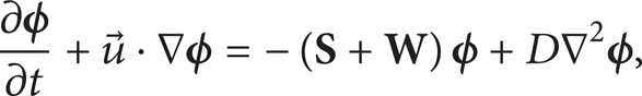
The modified Navier-Stokes equation after introducing of elastic stress term is as follows:

$\rho \left(\frac{\partial \overrightarrow{u}}{\partial t}+\overrightarrow{u}·\nabla \overrightarrow{u}\right)=-\nabla p+\mu {\nabla }^{\mathrm{2}}\overrightarrow{u}+\nabla ·{\tau }_p,$

(2)

where p is the pressure field and μ is viscosity of the Newtonian solvent. The elastic stress term τ _p is to be presented in the constitutive equation of viscoelastic fluid, which depicts the relationship between the micromolecules’ deformation and the elastic stress. And this this relationship reads

${\tau }_p=\frac{\left(\mathbf{C}-\eta \mathbf{I}\right)}{\lambda },$

(3)

where C is the conformation tensor of flexible molecules, I is the unit tensor, η is the viscosity of the elastic part, and λ is the relaxation time of viscoelastic fluid, respectively. By introducing the Giesekus constitutive model, the elastic term is then connected to the flow field; that is,

${\tau }_p+\lambda [\frac{\partial {\tau }_p}{\partial t}+\overrightarrow{u}·\nabla {\tau }_p-{\tau }_p·\nabla \overrightarrow{u}-\nabla {\overrightarrow{u}}^T·{\tau }_p+\frac{\alpha }{\eta }\left({\tau }_p·{\tau }_p\right)]=\eta \left(\nabla \overrightarrow{u}+\nabla {\overrightarrow{u}}^T\right),$

(4)

where α≠0 is the mobility factor and a value of 0.001 is used in the numerical computation.

For the passive scalars θ being transported along with the flow, they are depicted by

$\frac{\partial \theta }{\partial t}+\overrightarrow{u}·\nabla \theta =D{\nabla }^{\mathrm{2}}\theta ,$

(5)

where D is the diffusion coefficient of fluids.

2.2. Computing Domain and Nondimensional Procedures

The model for numerical simulation is one unit of curvilinear microchannel, as displayed in Figure 1, where periodic condition is used for both streamwise and spanwise directions, and radial direction is confined by the upper and lower no-slip walls. In the Cartesian coordinates, the dimensions of the geometry is nondimensionally set, with the range of [− 4, 4] in x direction, [− 4, 4] in y direction, and [0, 4] in z direction, respectively, and the computing domain is meshed by 64 × 64 × 64 grids. The computation is hereby carried out in a manner of that in Cartesian coordinates.

Figure 1:

The computational model of curved channel flow.

The height of the channel is defined between the walls, as 2H. Hereby, parameters of the half-height H, mean friction velocity $u_{\tau }={({\tau }_w/\rho )}^{\mathrm{1}/\mathrm{2}}$ , time scale H/u_τ, and pressure scale ρu_τ² are utilized to work out the nondimensional variables of length, velocity, time, and pressure involved in the computations; that is,

$\begin{array}{c}{\overrightarrow{x}}^{*}=\frac{\overrightarrow{x}}{H},\hspace{1em}\hspace{1em}{\overrightarrow{u}}^{*}=\frac{\overrightarrow{u}}{u_{\tau }},\hspace{1em}\hspace{1em}{t}^{*}=\frac{t}{\left(H/u_{\tau }\right)},\\ p^{*}=\frac{p}{\left(\rho {u_{\tau }}^{\mathrm{2}}\right)}={\stackrel{-}{p}}^{*}+p^{\prime *},\end{array}$

(6)

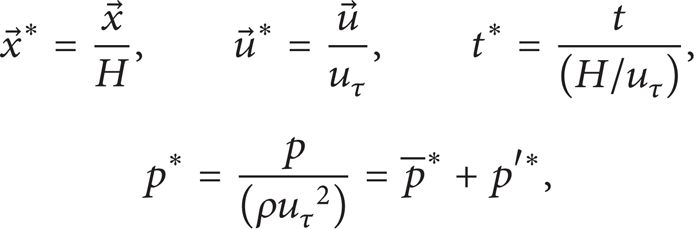
where τ _w is the mean wall shear stress on the entire wall and the nondimensionalized pressure p* is decomposed into average pressure part ${\stackrel{-}{p}}^{*}$ and the fluctuating pressure part p ^′* . With this method, $\partial {\stackrel{-}{p}}^{*}/\partial x$ is equal to unity along the geometry. As for conformation tensor, the nondimensional format is

${\mathbf{C}}^{*}=\frac{\mathbf{C}}{\eta }.$

(7)

For the nondimensional parameters appearing in as follows, such as Weissenberg number Wi_τ, Reynolds number Re_τ, Schmidt number Sc, Péclet number Pe, and ratio of solvent viscosity to solution viscosity β, are then defined as

$\begin{array}{c}\text{W}{\text{i}}_{\tau }=\frac{\lambda u_{\tau }}{H},\hspace{1em}\hspace{1em}\text{R}{\text{e}}_{\tau }=\frac{\rho u_{\tau }H}{\mu +\eta },\hspace{1em}\hspace{1em}\text{Sc}=\frac{\mu +\eta }{D},\\ \text{Pe}=\text{R}{\text{e}}_{\tau }·\text{Sc},\hspace{1em}\hspace{1em}\beta =\frac{\eta }{\mu +\eta }.\end{array}$

(8)

For convenience, Weissenberg number based on the nondimensional mean velocity U _m is also defined, read as Wi _m = U _m Wi_τ. According to the previous work [18], Wi_τ was regarded as the nominal Wi and Wi _m was the effective Wi that could be comparable with experiments.

Therefore, dropping the symbol “*”, the nondimensional governing equations for viscoelastic fluid flow and scalar transportation read as

$\nabla ·\overrightarrow{u}=\mathrm{0}$

(9)

$\frac{\partial \overrightarrow{u}}{\partial t}+\overrightarrow{u}·\nabla \overrightarrow{u}=-\nabla p^{\prime }+\frac{\beta }{\text{R}{\text{e}}_{\tau }}{\nabla }^{\mathrm{2}}\overrightarrow{u}+\frac{\mathrm{1}-\beta }{\text{R}{\text{e}}_{\tau }·\text{W}{\text{i}}_{\tau }}\nabla ·\left(\mathbf{C}-\mathbf{I}\right)-\nabla \stackrel{-}{p},$

(10)

$\frac{\partial \mathbf{C}}{\partial t}+\overrightarrow{u}·\nabla \mathbf{C}=\mathbf{C}·\nabla \overrightarrow{u}+\nabla {\overrightarrow{u}}^T·\mathbf{C}-\frac{\left[\mathbf{I}+\alpha \left(\mathbf{C}-\mathbf{I}\right)\right]·\left(\mathbf{C}-\mathbf{I}\right)}{\text{W}{\text{i}}_{\tau }}+\kappa {\nabla }^{\mathrm{2}}\mathbf{C}\mathbf{,}$

(11)

$\frac{\partial \theta }{\partial t}+\overrightarrow{u}·\nabla \theta =\frac{\mathrm{1}}{\text{Pe}}{\nabla }^{\mathrm{2}}\theta .$

(12)

For the computation of scalar transportation, (12) is taken into calculation after the flow reached the numerically steady status. Specifically, the scalar θ is initially set to be 0 and 1 for the upper and lower half channel, respectively (also shown in Figure 5 later). And as time marching, it evolves with the deformation of carrier flow.

2.3. Numerical Procedures

An at least second-order difference method is adopted to discretize the differential equations. For spatial variables, the convective term and the conformation tensor transportation equation, the QUICK scheme, and MINMOD scheme are utilized, respectively. And for time-related terms, the second-order Crank-Nicholson method is used, and the time step is set as 10⁻⁵. Also an artificial diffusion term κ∇²C (κ is the relaxation factor) is added in (11) to eliminate the solution unsteadiness, where a sufficiently small artificial coefficient (less than 10⁻³) does not qualitatively change the flow behaviors [19].

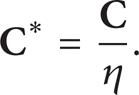
For the specific flow conditions, the details are listed in Table 1.

Table 1:

Numerical cases and relative parameters.

Cases	Reτ	Wiτ	β	α	κ	$\nabla \stackrel{-}{p}$
Newtonian fluid	1	0	—	—	—	−1
Viscoelastic fluid	1	0.5, 1, 2, 3, 5, 10, 20 35, 50, 80, 100, 150, 200, 300, 500	0.25	10−3	10−3	−1

3. Results and Discussions

In an early experimental study on the irregular flow field in the curvilinear microchannel, Li et al. [20] have shown the velocity distributions at the different planes along depth direction by micro-PIV measurement, indicating that a disordered flow state develops for the viscoelastic fluids even at an ultralow flow rate. The previous DNS study [18] on the elastic instability inception and development has clearly explained the chaotic state started at a critical Weissenberg number of about 2, after that the friction factor C _f = 2/U _m ² grew sharply due to the generation of unstable secondary flow in the cross-section, where the secondary flow was perpendicular in the streamwise direction [18]. For the carried scalars, the temporal evolution of the ensemble root mean square (rms) of concentration decays exponentially, being excellently consistent with the experimental results [3]. Consequently, while the contribution of viscous effect on the kinetic energy (also mixing effect) maintained at low level, the elastic effect contribution predominated the flow and the inertial effect kept approximately zero. That could suggest that the flow almost depended on the motion of the flexible long-chain molecules of the solute, such as the stretching by the flow and curling or oscillating by the geometry. This would be the premise of the current work, since the scalar motion is completely dependent on the flow structures.

3.1. Flow Structures

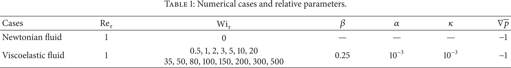
To illustrate how the scalar behaves in the elastically chaotic flow, the flow structures should pay special attention at the outset. The substantial stretching of the flexible long-chain molecules will be attained as the flow state turns more irregular. This can be depicted by the trace of the molecular conformation tensor tr⁡(C) = C₁₁ + C₂₂ + C₃₃ in the whole flow field. As presented in Figure 2, both the ensemble average value and the maximum value of trace come to a sudden augment around Wi _m ~2, and so was the ratio of elastic stress to viscous stress. With the maximum value of the trace, the strong extension emerges close to the inner wall with the small radius of curvature, where the sign of curvature shifts. Intensive stretching arising out of the great local velocity gradient near the wall gives birth to the “energy transfer” into the bulk. Thus a rational deduction is that the extended long-chain molecules will be flung into the center of channel after they are stretched to break, and if not, they should burst into the bulk with a certain frequency according to the fluid properties and flow conditions. It is worth noticing that a quasiperiodic unsteady flow in the cross-section by the previous numerical study is in accordance with the analysis above [18]. Furthermore, this is actually observed in the experiments by using a CTAC/NaSal solution flow in such a serpentine curved microchannel (experimental settings can be found in [21]), as displayed in Figure 3. Note the bright stripes carry the passive scalars, directly exhibiting the motions of flow inside. The flow conditions in the experiments have a range of Wi around 7.5~15. As for simulation, a critical Wi _m ~2 is found over which the flow turns into irregular state. Thus these flow conditions are in comparable range; hereby, both simulations and experiments imply that scalar evolution is coherent with deformation of the viscoelastic molecules.

Figure 2:

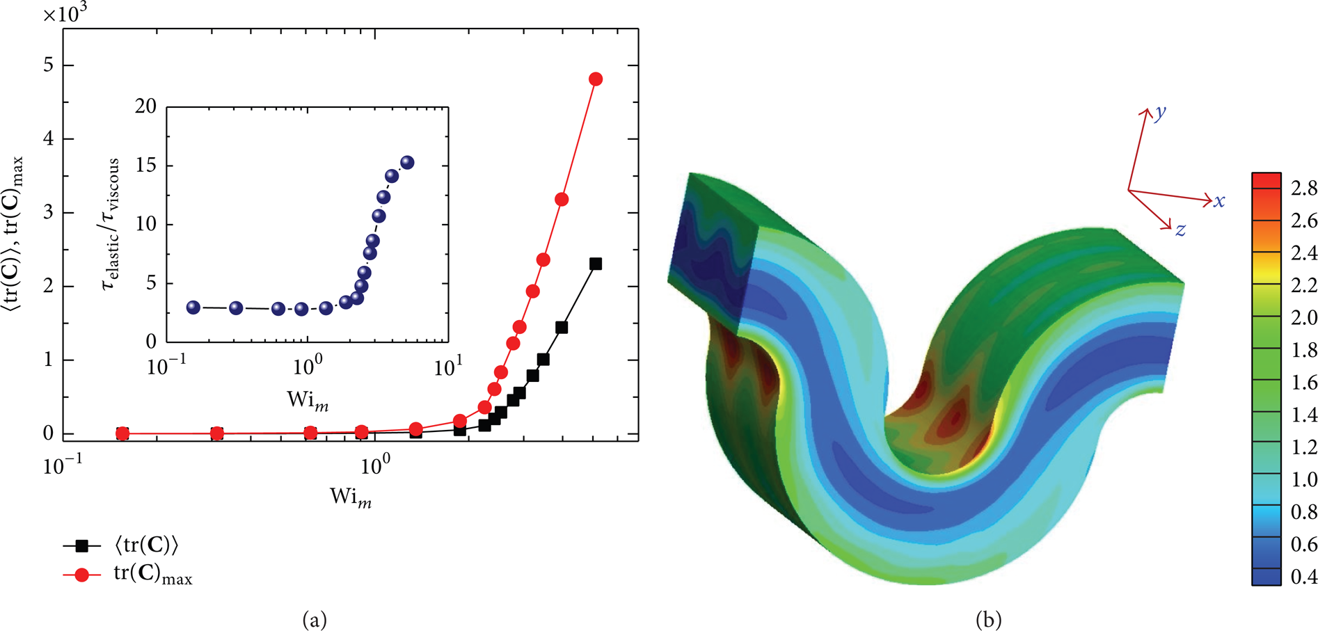
Extension of flexible molecules versus Wi; inset is the relative importance of elastic stress to viscous stress. The right is the extension contour for the flow field, tr⁡( C )/〈tr⁡( C )〉; flow condition: Wi_τ = 100.

Figure 3:

Illustration of stretched stripes near the inner wall.

Along with the strong extension of viscoelastic fluid, the fluctuation of scalar concentration in the spatial field would be affected at various length scales. This can be illuminated by the decay of the two-dimensional scalar spectral function E_θ(k). According to Williams et al. [22], it is defined as

$E_{\theta }\left(k\right)=\mathrm{2}\pi k\Delta \left(k\right),$

(13)

where $\Delta \left(k\right)=\Delta \left(\overrightarrow{k}\right)$ is the two-dimensional energy spectrum of scalar field $\theta \left(\overrightarrow{x}\right)$ , if the scalar distribution is statistically stable, and it read as

$\Delta \left(\overrightarrow{k}\right)={\left(\frac{\mathrm{2}\pi }{a}\right)}^{\mathrm{2}}{\left|\Theta \left(\overrightarrow{k}\right)\right|}^{\mathrm{2}}.$

(14)

Therein, $\Theta \left(\overrightarrow{k}\right)$ is the Fourier transformation of $\theta \left(\overrightarrow{x}\right)$ and is the size of field of view and k is the wave number. Therefore, we could establish the scalar spectral function decay from the scalar field by experiments, and it is presented in Figure 4.

Figure 4:

Scalar power spectra by experiments in the wave number domain at different flow units (a), and the fling stripes in the burst events (b). Flow condition is about Pe = 4.78 × 10⁷.

Figure 5:

Scalar and scalar gradient for initial condition (t = 0).

Figure 4(a) displays the experimental results of scalar power spectra, where N represents the different flow units along the flow direction. As the flow gets fully developed, they show the similar decay in the space. One could identify the scalar spectra function decay with an exponential index of −0.95, which fairly agrees with the theoretical value of −1 predicted by Batchelor and Kraichnan [23, 24]. However, it should be noticed that the scalar spectra decay shows wiggles at the small wave number region, implying the stretched stripes with concentrated scalars fling in the bulk flow, according to relatively large-scale motion. This can also be explained by the fling motion as shown in Figure 4(b). In the experiments, the time-dependent motion of stripes is from strongly extended long-chain molecules where the fluorescent particles (scalars) concentrate. They are captured by using a high-speed CMOS camera. It can be seen that these stripes are mainly extended near the region of small curvature radius. The curved stripes are showing the fling motion from near-wall region to the bulk, and they have a quasiperiodic behavior. The above finding is consistent with the simulation results presented above.

3.2. Scalar Gradient Structures

To calculate the gradient for (5), one can get

$\frac{\partial \mathit{\varphi }}{\partial t}+\overrightarrow{u}·\nabla \mathit{\varphi }=-\left(\mathbf{S}+\mathbf{W}\right)\mathit{\varphi }+D{\nabla }^{\mathrm{2}}\mathit{\varphi },$

(15)

where ϕ = ∇θ is the scalar gradient and $\mathbf{S}=(\nabla \overrightarrow{u}+\nabla {\overrightarrow{u}}^T)/\mathrm{2}$ and $\mathbf{W}=(\nabla \overrightarrow{u}-\nabla {\overrightarrow{u}}^T)/\mathrm{2}$ are the strain rate tensor and rotation tensor of flow field, respectively. The information of the scalar gradient ϕ immediately expresses the uniformity of the scalar distribution promoted by the “energy transfer” effect. To begin with, Figure 5 gives the initial conditions for the scalar concentration and the scalar gradient at t = 0. The scalars are set as 1 and 0 for the lower half part and upper half part, respectively; therefore, as an initial state, the scalar gradient only happens at the centerline of the flow field. This boundary condition of scalar distribution holds the same for both Newtonian fluid and viscoelastic fluid cases. Note that the scalar transportation computation is introduced after the flow becomes developed, so the scalar motion is always transported by the fully developed flow.

In Figure 6, the contours represent the temporal evolutions of scalar concentration under some certain flow conditions, where the parameter t indicates the nondimensional computation time. As for a Newtonian fluid (Wi_τ = 0), the carried scalars are in the motion of diffusion. The interface between the two layers of differently concentrated scalars becomes smearing, while the newly generated layers remain parallel along the flow direction. There is no spanwise motion found for all the time instant. In contrast, for a viscoelastic fluid flow, its state is dominated by the convection effect, and the scalars are promptly transported by the vortices to reach uniform distribution in the whole geometry. The flow components both in spanwise direction and radial direction are much stronger than Newtonian case, and scalar motion is quite fast.

Figure 6:

Scalar contour versus time at different flow conditions.

Comparing with the previous work on the flow structures [18], it is obvious that the evolution of secondary flow structures show the similar features with that of scalar transportation. For the flow inside the curved channel, the new vortex structures with opposite rotating directions continuously generate near the wall and then move to the opposite walls. It would imply that the scalar is effectively transported with such irregular flow. Thus the scalar gradients in the flow geometry should relate to these special flow structures.

Accordingly, the scalar gradient evolution is visualized in the forms of isosurfaces of |ϕ| (Figure 7), both with full range of gradient value and a cut-off threshold of two times of average gradient value TH = 2〈|ϕ|〉 (TH represents the threshold). As expected, stratified patterns of scalar gradient form for the Newtonian fluid flow. In consequence of long-time decay, they transform into dispersively fine granular structures. This is apparently dissimilar to that in the developed turbulence flow and indicates that the decay of scalar gradient driven by diffusion seems much local in its motion. For viscoelastic fluid, the scalar gradient structures shape into closed curved surfaces or tubes, which subsequently change into flat tubes and then long stripes. These structures are different from that found in the developed inertial turbulence [17]. In inertial channel turbulence, the scalar gradients evolve into thin layer structures. Thus the motion and deformation of viscoelastic fluid are crucially responsible for the scalar gradient structures, and this will be addressed in the next section.

Figure 7:

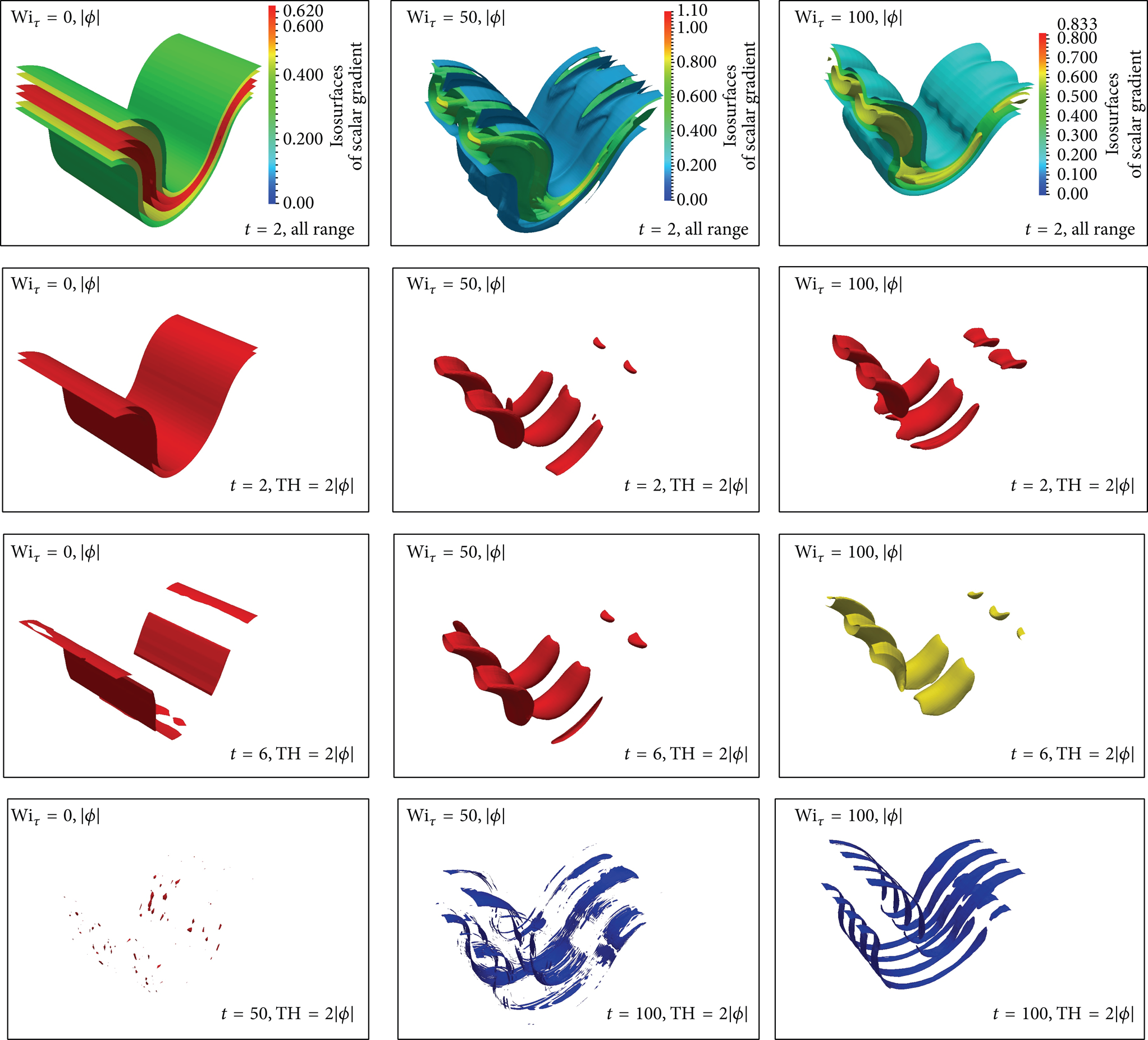
Scalar gradient structures versus time at different flow conditions. The isosurfaces are set to all range of scalar gradient magnitude and 2 times mean value of their magnitude as threshold (TH = 2〈|ϕ|〉), respectively.

As a whole, the scalar gradient evolves as follows in a confined elasticity-induced chaotic flow. The structures of the scalar gradient initiate from the closed surfaces in the center which are characterized by the vortices’ development (rolling) and then are extended in streamwise direction and compressed in radial direction by the carried flow. When the isosurfaces with large scalar gradient vanish in the bulk, some remain near the wall boundaries. That means that the scalars are transported universally by flow extension and rotation movements in the microchannel and finally concentrated at places where the shear effect dominates. Moreover, the thin threads of scalar gradient are probably a result of microstructure stretching effect, relating with the flow structures.

3.3. Characteristics of Microstructures

From the discussion above, the flow structures and the deformation of flexible molecules should be to a certain extent connected to each other. It is worth investigating such a relationship by using the probability distribution function (PDF) analysis between micromolecular conformation tensor C (with eigenvectors a _i ) and flow field strain rate tensor S (with eigenvectors e _i ). Those PDFs look into the parallelism of corresponding eigenvectors of two tensors, to an extent indicating the correlation of two variables. At first the eigenvectors are calculated from the tensors for the whole flow field and then the cosine of the angles between those eigenvectors are computed for PDF analysis.

Figure 8 displays the PDFs of cosine value of the angles between eigenvectors e _i and a _i . The results seem to be not well related since both $({\mathbf{e}}_{\mathbf{1}},{\mathbf{a}}_{\mathbf{1}})$ and $({\mathbf{e}}_{\mathbf{2}},{\mathbf{a}}_{\mathbf{2}})$ are perpendicular to each other, respectively, and $({\mathbf{e}}_{\mathbf{3}},{\mathbf{a}}_{\mathbf{3}})$ mainly make an angle of 45 degrees. Indeed, strong secondary flow in the cross-section perpendicular to the streamwise primarily contributes to the flow rotation motion $\left({\mathbf{e}}_{\mathbf{2}}\right)$ , while long-chain molecules are in major stretching along the streamwise direction $\left({\mathbf{a}}_{\mathbf{1}}\right)$ . This finding reveals that the molecular deformations do not directly evoke the flow instabilities or turbulence in this case but through the variation and confinement of geometry; that is, they are weakly correlated with the deformations of flow field. In particular, in a homogenous isotropic turbulence excited by elasticity, (e _i ,a _i ) should be remarkably correlated [25]. Concerning the scalar transportation, thus, the fast evolution attributes to elastically enhanced secondary flow.

Figure 8:

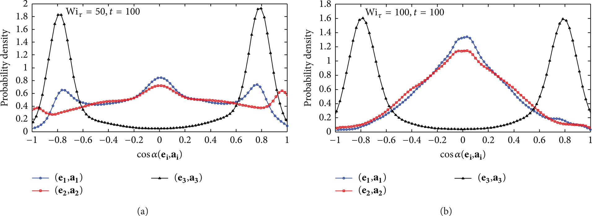
PDFs of cosine of the angles between eigenvectors e _i and a _i .

To further elucidate this viewpoint, the relationship between the vorticity ω and the molecular deformation were also presented as in Figure 9. The primary molecular stretching direction $\left({\mathbf{a}}_{\mathbf{1}}\right)$ is mainly in parallel and antiparallel configuration with the flow vorticity. Meantime, the molecular stretching in the other directions ( ${\mathbf{a}}_{\mathbf{2}}$ and ${\mathbf{a}}_{\mathbf{3}}$ ) is in small quantity and mainly perpendicular to the vorticity direction. Since the vorticity direction is perpendicular to the vortex, thus, it can be deduced that the stretched long-chain molecules devote largely to the chaotic flow.

Figure 9:

PDFs of cosine of the angles between eigenvectors a _i and vorticity ω.

As an interesting side, we would like to investigate how the scalar gradients correlate with velocity vectors, as shown in Figure 10. It suggests that the direction of velocity is always orthogonal to the scalar gradient. Since the scalars are carried by the fluid motion, the scalars transportation speed changes at different velocity layers. Therefore, in this shear-dominated flow, the scalar gradients turn out the layer structures. As passively transported by the vortices of secondary flow, they form a closed tube appearance in the center of channel.

Figure 10:

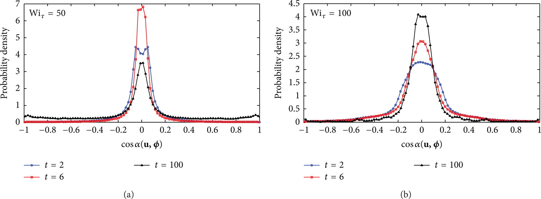
PDFs of cosine of the angles between velocity vectors u and scalar gradients ϕ.

4. Conclusion

In summary, this work focuses on the passive particle motion in an irregular flow with viscoelastic fluid. Purely elasticity-induced chaotic flow and scalar mixing in the curvilinear microchannel has been investigated by a three-dimensional DNS study. The scalar evolution characteristics are well consistent with the experimental findings. For the structures of scalar gradients, their isosurfaces vary from “rolls” in the bulk to “threads” near the wall. The weak correlation between micromolecular deformation and flow field deformation tend to imply the importance of geometry layout. And the strong secondary flow again indicates stretching of viscoelastic micromolecules works as a medium for the enhancement of scalar transportation in the flow field. With the analysis on the PDFs of eigenvectors’ parallelism, the mechanism for scalar evolution, molecules’ stretching, and the scalar gradients’ structures are elucidated.

Conflict of Interests

The authors declare that there is no conflict of interests regarding the publication of this paper.