Sage Journals: Discover world-class research

Abstract

Camera robots are high-speed redundantly cable-driven parallel manipulators that realize the aerial panoramic photographing. When long-span cables and high maneuverability are involved, the effects of cable sags and inertias on the dynamics must be carefully dealt with. This paper is devoted to the optimal cable tension distribution (OCTD for short) of the camera robots. Firstly, each fast varying-length cable is discretized into some nodes for computing the cable inertias. Secondly, the dynamic equation integrated with the cable inertias is set up regarding the large-span cables as catenaries. Thirdly, an iterative optimization algorithm is introduced for the cable tension distribution by using the dynamic equation and sag-to-span ratios as constraint conditions. Finally, numerical examples are presented to demonstrate the effects of cable sags and inertias on determining tensions. The results justify the convergence and effectiveness of the algorithm. In addition, the results show that it is necessary to take the cable sags and inertias into consideration for the large-span manipulators.

1. Introduction

In the recent years, redundantly cable-driven parallel camera robots (camera robots for short, see Figure 1) have been developed for the increasing requirements of the aerial panoramic photographing [1]. Besides the camera robots, rocker cameras, crank arm lift trucks, and helicopters are often employed for the aerial panoramic photographing. However, rocker cameras and crank arm lift trucks suffer from the limited shooting angles and interrupt audience's view of scene; helicopter shootings are subject to the vibration, noise, and expensive cost. Thanks to the camera robots, it is easy to take pictures from some perspectives that a conventional camera cannot achieve [2], leading to the convenient realization of the large range of aerial panoramic photographing.

Figure 1:

Schematic of a camera robot configuration.

When a camera robot works normally, its speed and acceleration may be considerately great. Thus, a proper and exact OCTD is essential for guaranteeing its stable operation. Many researchers have investigated the OCTD problem. Hassan and Khajepour [3] presented a method based on convex theory for the OCTD. Pott et al. [4] developed a closed-form OCTD algorithm. Borgstrom et al. [5] computed the safe tensions through a linear program by introducing a slack variable. Gosselin and Grenier [6] presented a noniterative algorithm of OCTD. But all of these OCTD algorithms are not applicable to the camera robot. Furthermore, the cables in the above literature are all regarded as massless straight lines due to the small-dimension size of the manipulators. For a camera robot, this assumption is invalid owing to the sags caused by the nonnegligible self-mass of the large-span cables [7]. The effects of the cable sags on the kinematics and dynamics must be taken into account for large-span cables [8 –13].

Yao et al. [14] approximated the catenary as a parabola for a four-cable-driven parallel manipulator of the large radio telescope. Gouttefarde et al. [15] explored a simplified approach for the large-dimension cable-driven manipulator. Du et al. [16] presented a simple dynamic modeling approach of large workspace cable-driven parallel manipulators. However, these works only involve the end-effectors’ inertias without taking cable inertias into consideration. Du et al. [17] studied the large-span cable dynamics through the finite element method. Nevertheless, the cable inertias are not considered completely due to the slow motions and the manipulator is not driven redundantly. For a large-span cable-driven manipulator, it cannot achieve the desired control effects for force or force/position control without considering cable inertias and sags, especially in the case of high-speed motions.

Compared with the manipulators in the above literature, the camera robots offer three obvious features. (1) Due to the large-span cables, the sags must be taken into consideration. (2) Because of the high maneuverability, the cable inertias cannot be ignored. (3) Owing to the redundant actuation, the tension distribution among the cables does not have the unique solution. The three features lead to a difficulty in determining the OCTD, which motivates the research on the OCTD of the camera robot in this paper. Since the cable sags and inertias have all nonnegligible effects on dynamics, we establish the dynamic equation combined with both the cable sags and inertias. In order to find the unique solution to cable tension distribution, an iterative optimization algorithm is introduced based on the dynamic equation.

The paper is organized as follows. Section 2 describes the camera robot. The dynamic equation of the camera robot is set up in Section 3. In Section 4, an optimization model for the cable tension distribution is established. In Section 5, an iterative optimization algorithm is introduced. Section 6 verifies the effectiveness of the algorithm and illustrates the necessity of taking the cable sags and inertias into account. Finally, Section 7 concludes this paper.

2. Description

2.1. Description of the Camera Robots

In order to fully control the motion of a camera robot, redundant actuation must be employed [18]. The camera robot structure is displayed in Figure 1, consisting of a moving camera platform with 3 translational DOF driven by four cables. The four cables are connected to the four pulleys, which are attached to the ceiling of masts, respectively. The camera platform moves freely in any direction because the cables can be shortened and lengthened controlled by four servomotors according to the commands sent from the central controller.

By means of a composite hinge structure, the demand for translation and rotation decoupling of the camera platform can be satisfied, so the camera platform can look like an ideal mass point. A global fixed frame, noted as {Oxyz}, is attached to the ground as shown, where O is the origin point. $P = {(x_{p}, y_{p}, z_{p})}^{T}$ is a position vector representing the position of the camera platform in {Oxyz}. Point B _i, at which thecable i (i = 1, 2, 3, 4) is tangent to the pulley, isassumed to be fixed to the global fixed frame. Obviously, vectors $B_{i} = {[B_{i, x}, B_{i, y}, B_{i, z}]}^{T}$ are constant position vectors connecting O to B _i in {Oxyz}.

2.2. Catenary Equation of the Cable

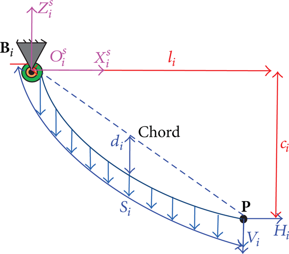
In order to guarantee the normal work of the camera robot, the cables must offer high strength and elastic modulus. As a result, the cables are inextensible. As shown in Figure 2, a local cable frame, noted as {o_i^sx_i^sz_i^s}, is attached to B _i, in which the z^s axis of the cable frame points in the same direction with the global z-axis.

Figure 2:

Catenary cable i in its vertical plane.

The catenary equation can be applied for describing the profile of the cable under the sag influence. When the camera robot works normally, the camera platform moves stably. As a consequence, the profile of the cable i is the catenary within the o^sx^sz^s plane, which can be expressed as follows [19]:

z_{i}^{s} = \frac{H_{i}}{ρ g} [\cosh α_{i} - \cosh (\frac{2 β_{i} x_{i}^{s}}{l_{i}} - α_{i})],

(1)

where x_i^s and z_i^s are x- and z-direction coordinates in {o_i^sx_i^sz_i^s}; ρ is linear density of the inextensible cable; g = 9.8 m/s² is the gravitational acceleration with the direction along the negative direction of the z-axis; α_i = sinh⁡₋₁⁡[β_i(c_i/l_i)/sinh⁡⁡β_i] + β_i, β_i = ρgl_i/2H_i; H_i and V_i are the horizontal and vertical components of each cable tension at the cable end P ; l_i and c_i are the horizontal and vertical spans of each cable, respectively. The length of the cable S_i can be calculated as follows:

S_{i} = \sqrt{1 + {(\frac{d z_{i}^{s}}{d x_{i}^{s}})}^{2}} = l_{i} - \frac{H_{i} β_{i}}{ρ g l_{i}} [\frac{l_{i}}{16 β_{i}} (e^{4 β_{i} - 2 α_{i}} - e^{- 4 β_{i} + 2 α_{i}}) + \frac{1}{2}] .

(2)

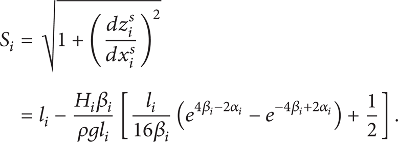
The corresponding sag d_i is

d_{i} = \frac{8 H_{i} \sinh β_{i} \sinh^{- 1} ((ρ g c_{i} / 2 H_{i}) / \sinh β_{i}) - c_{i} ρ g}{2 ρ g} .

(3)

It can be found from (3) that the sag depends on H_i. In practical applications, the sag-to-span ratio is often employed for evaluating tautness of the cable. In order to ensure the normal work of camera robot, the cable should be kept as taut as possible. Namely, the sag-to-span ratio is as small as possible.

3. Dynamics of the Camera Robot

3.1. Dynamics of a Fast Varying-Length Cable

As shown in Figure 3, the cable is equally divided by n nodes with the cable length S_i. Thus, the distance between any two adjacent nodes r_i = S_i(t)/(n − 1), in which S_i(t) is the time-varying length of the corresponding cable i. Let {B_is_i} be the curve length frame of cable i, in which s_i is the curve length away from B _i. The p_ij (j = 1, 2, …,n) is the jth node on the cable i, whose curve length away from B _i is s_ij(t) at time t, in which t is the time variable (s_ij(t) is abbreviated to s_ij in this section). For each cable, the end node p_i1 is fixed at B _i with s_i1 = 0 and p_in is connected to the camera platform P commonly with s_in = S_i. Denote the position vector of the node p_ij by $q_{i j} (s_{i j}, t) = {[x (s_{i j}, t), y_{i j} (s_{i j}, t), z_{i j} (s_{i j}, t)]}^{T}$ ; τ(s_ij,t) is the unit vector tangent to the node p_ij. q _ij(s_ij,t) and τ(s_ij,t) are all the functions with regard to the curve length coordinate s_ij and the time variable t.

Figure 3:

A cable with the discrete nodes.

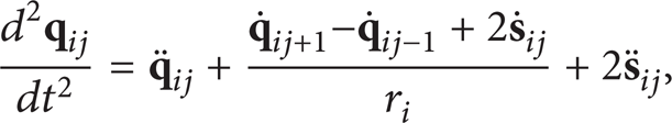
As shown in Figure 4, the motion of p_ij is composed of the spatial motion and the axial motion with the cable length variations [16]. Due to the high maneuverability of the camera robot, the cable lengths change rapidly. Hence, the cable's axial velocity and acceleration cannot be ignored, leading to the nonnegligible inertia. For simplification, q _ij(s_ij,t) is abbreviated to q _ij for (5)–(9). As a result, the governing equation of inertia for a node p_ij is given by [11, 16]

ρ \frac{d^{2} q_{i j}}{d t^{2}} \partial s_{i} = \frac{\partial}{\partial s_{i}} [σ (s_{i j}, t) τ (s_{i j}, t)] + W_{e} (s_{i j}, t) - ρ g d s_{i},

(4)

where σ(s_ij,t) is the cable tension at node j; $τ (s_{i j}, t) = {(τ_{i j x}, τ_{i j y}, τ_{i j z})}^{T}$ is the unit vector of the tangent at node p_ij; $W_{e} (s_{i j}, t) = {[W_{e x}, W_{e y}, W_{e z}]}^{T}$ is the external force per unit length of the cable. In this paper, W _e(s_ij,t) = [000]^T.

Figure 4:

The motion of p(s_ij,t) on cable i.

The velocity and acceleration of the node p_ij can be calculated by taking the first and second derivatives of q _ij with respect to time t in the following expression, respectively [16]:

\begin{matrix} \frac{d q_{i j}}{d t} = \frac{\partial q_{i j}}{\partial t} + \frac{\partial q_{i j}}{\partial s_{i j}} {\dot{s}}_{i j} \end{matrix}, \begin{matrix} \frac{d^{2} q_{i j}}{d t^{2}} = \frac{\partial^{2} q_{i j}}{\partial t^{2}} + 2 \frac{\partial^{2} q_{i j}}{\partial s_{i j} \partial t} + \frac{\partial^{2} q_{i j}}{\partial s_{i j}^{2}} {\dot{s}}_{i} + \frac{\partial q_{i j}}{\partial s_{i j}} {\ddot{s}}_{i j}, \end{matrix}

(5)

where ${\dot{s}}_{i j} = d s_{i} / d t$ and ${\ddot{s}}_{i j} = d^{2} s_{i} / d t^{2}$ . ∂² q _ij/∂t² is caused by the cable's spatial motion; $(\partial q_{i j} / \partial s_{i j}) {\ddot{s}}_{i j}$ is caused by the cable's axial motion; ∂² q _ij/∂s_ij∂t and $(\partial^{2} q_{i j} / \partial s_{i j}^{2}) {\dot{s}}_{i}$ are caused by the cable's both spatial and axial motions. The first and second derivatives of q _ij(s_ij,t) with respect to the curve length coordinate s_ij can be obtained as follows:

\begin{matrix} \frac{\partial q_{i j}}{\partial s_{i j}} = \frac{q_{i j + 1} - q_{i j - 1}}{2 r_{i}}, \\ \frac{\partial q_{i j}}{\partial s_{i j} \partial t} = \frac{{\dot{q}}_{i j + 1} - {\dot{q}}_{i j - 1}}{2 r_{i}}, \\ \frac{\partial^{2} q_{i j}}{\partial s_{i j}^{2}} = \frac{q_{i j + 1} - 2 q_{i j} - q_{i j - 1}}{r_{i}^{2}}, \end{matrix}

(6)

where ${\dot{q}}_{i j} = \partial q_{i j} / \partial t = ({\dot{q}}_{i j} (s_{i j}, t + Δ t) - {\dot{q}}_{i j}) / Δ t$ , in which Δt is the tiny time increment. The motion direction of cable length variation at node p(s_ij,t) can be regarded as the direction of tangent τ(s_ij,t). Since the cable is inextensible, there is no relative motion between any two cable nodes. As a result, ${\dot{s}}_{i j} = {\dot{S}}_{i} τ (s_{i j}, t)$ and ${\ddot{s}}_{i j} = {\ddot{S}}_{i} τ (s_{i j}, t)$ ; $∥ {\dot{s}}_{i j} ∥ = Δ {\dot{S}}_{i} / Δ t$ and $∥ {\ddot{s}}_{i j} ∥ = Δ {\ddot{S}}_{i} / Δ t$ . Suppose that the cables of the camera robot offer small sag-to-span ratio and then ∥( q _{ij + 1} − q _{ij − 1})/2r_i∥ ≈ 2 and ∥( q _{ij + 1} − 2 q _ij − q _{ij − 1})/r_i²∥ ≈ 2/r_i. Substitute (6) into (5), and simplify

\frac{d^{2} q_{i j}}{d t^{2}} = {\ddot{q}}_{i j} + \frac{{\dot{q}}_{i j + 1} - {\dot{q}}_{i j - 1} + 2 {\dot{s}}_{i j}}{r_{i}} + 2 {\ddot{s}}_{i j},

(7)

where ${\ddot{q}}_{i j} = \partial^{2} q_{i j} / \partial t^{2} = {\dot{q}}_{i j} / Δ t$ . Let T _i = σ(S_i,t)τ(S_i,t) be the tension of cable i along the tangent direction at the cable end node P . Noting that the left side of (4) denotes the inertia of p_ij caused by cable's motion, thus integrating (4) with respect to s_i leads to the following dynamic equation for the inertia of the whole cable:

ρ \sum_{j = 1}^{n} ({\ddot{q}}_{i j} + \frac{{\dot{q}}_{i j + 1} - {\dot{q}}_{i j - 1} + 2 {\dot{s}}_{i j}}{r_{i}} + 2 {\ddot{s}}_{i j}) d s_{i} = \int_{0}^{S_{i}} \frac{\partial}{\partial s_{i}} σ (s_{i j}, t) τ (s_{i j}, t) d s_{i} - \int_{0}^{S_{i}} ρ g d s_{i} .

(8)

By noting that ∥ds_i/r_i∥ = 1, ${σ (s_{i j}, t) τ (s_{i j}, t) |}_{0}^{S_{i}} = T_{i}$ , $\int_{0}^{S_{i}} d s_{i} = S_{i}$ , and ∑_{j = 1}ⁿds_i = S_i. (8) can be further reduced to

ρ \sum_{j = 1}^{n} S_{i} (p_{va} + {2 S}_{va}) = T_{i} - ρ g S_{i},

(9)

where $p_{v a} = {\ddot{q}}_{i j} + ({\dot{q}}_{i j + 1} - {\dot{q}}_{i j - 1}) / S_{i} = {(q_{i j x}, q_{i j y}, q_{i j z})}^{T}$ ; $S_{va} = {\dot{s}}_{i j} / S_{i} + {\ddot{s}}_{i j} = {(s_{i j x}, s_{i j y}, s_{i j z})}^{T}$ .

3.2. Dynamic Equation of the Camera Robot

The cable tension T _i at the cable end node P (i.e., the camera platform) can be written in terms of $T_{i} = {[H_{i} \cos θ_{i} H_{i} \sin θ_{i} H_{i} \tan γ_{i}]}^{T}$ . θ_i is the angle between x^s in {o^sx^sz^s} and x-axis in {Oxyz}; V_i = H_itanγ_i; γ_i is the angle between H_i and T _i. As shown in Figure 5, the tension T _i is decomposed into the x-, y-, and z-directions at P , and then the dynamic equation of the camera robot system can be written as follows:

\begin{matrix} m_{p} {\ddot{x}}_{p} + 2 ρ \sum_{i = 1}^{4} \sum_{j = 1}^{n} (q_{i j x} + s_{i j x}) \cos θ_{i} = \sum_{i = 1}^{4} H_{i} \cos θ_{i} + f_{e, x}, \\ m_{p} {\ddot{y}}_{p} + 2 ρ \sum_{i = 1}^{4} \sum_{j = 1}^{n} (q_{i j y} + s_{i j x}) \sin θ_{i} = \sum_{i = 1}^{4} H_{i} \sin θ_{i} + f_{e, y}, \\ m_{p} {\ddot{z}}_{p} + 2 ρ \sum_{i = 1}^{4} \sum_{j = 1}^{n} (q_{i j z} + s_{i j x}) \tan γ_{i} = \sum_{i = 1}^{4} H_{i} \tan γ_{i} - \sum_{i = 1}^{4} ρg S_{i} - m_{p} g + f_{e, z}, \end{matrix}

(10)

where $a = {[{\ddot{x}}_{p}, {\ddot{y}}_{p}, {\ddot{z}}_{p}]}^{T}$ is the acceleration of the camera platform. Equation (10) can be written in the following matrix form:

M_{p} a + 2 J M_{c} \sum_{j = 1}^{n} (S_{va} + p_{va}) = J H - f_{g} - f_{G} + f_{e},

(11)

where $M_{p} = [\begin{smallmatrix} m_{p} & 0 & 0 \\ 0 & m_{p} & 0 \\ 0 & 0 & m_{p} \end{smallmatrix}]$ , m_p is the mass of the camera platform; $M_{c} = [\begin{smallmatrix} m_{c} & 0 & 0 \\ 0 & m_{c} & 0 \\ 0 & 0 & m_{c} \end{smallmatrix}]$ , m_c = ρ∑_{i = 1}⁴S_i is the total mass of the four cables. $H = {[\begin{bmatrix} H_{1} & H_{2} & H_{3} & H_{4} \end{bmatrix}]}^{T}$ is the vector describing horizontal components of all the cable tensions at the cable end P . f _g = ρg S ; $S = {[\begin{bmatrix} S_{1} & S_{2} & S_{3} & S_{4} \end{bmatrix}]}^{T}$ is the vector consisting of all the cable lengths. f _G ∈ R ³ is the gravitational force of the camera platform. f _e ∈ R ³ is the generalized external force on the camera platform. Up to now, (7) can be reduced to a simpler form:

J H = Q,

(12)

where Q = M _p a + f _cab + f _g + f _G − f _e; $J = {[J_{1} J_{2} J_{3} J_{4}]}_{3 \times 4}$ is the structure matrix of the camera robot; $J_{i} = {[\cos θ_{i} \sin θ_{i} \tan γ_{i}]}^{T} (i = 1,2, 3,4)$ ; f _cab = 2 JM _c∑_{j = 1}ⁿ( S _va + p _va), named as the cable inertia term.

Figure 5:

Components of a cable tensionat the cable end P .

4. Optimal Model of the Cable Tension Distribution

4.1. Cable Tension Distribution Equation

Because the camera robot is a redundant driven mechanism, the structure matrix J is not a square matrix. With the introduction of Moore-Penrose generalized inverse matrix J ⁺ of the structure matrix J , H can be determined from the following equation [5, 6, 18]:

H = H_{s} + H_{h},

(13)

where H _s is the special solution to the cable tension; H _h is the homogeneous solution to the cable tension; H _s and H _h are calculable as follows:

H_{s} = {[\begin{bmatrix} H_{s}^{1} & H_{s}^{2} & H_{s}^{3} & H_{s}^{4} \end{bmatrix}]}^{T} = J^{+} Q,

(14)

H_{h} = N (J) λ,

(15)

where $N = {[N_{1} N_{2} N_{3} N_{4}]}^{T}$ is the kernel of the matrix J , and λ is an arbitrary scalar. As Figure 5 shows, the vertical component of the tension at the cable end P of cable i is as follows:

V_{i} = H_{i} \tan γ_{i} (i = 1,2, 3,4) .

(16)

Thus, the cable tension of cable i at the cable end P is obtained from the following equation:

T_{i} = H_{i} \sqrt{1 + \tan^{2} γ_{i}} (i = 1,2, 3,4) .

(17)

4.2. Constrained Conditions of the Optimization Model

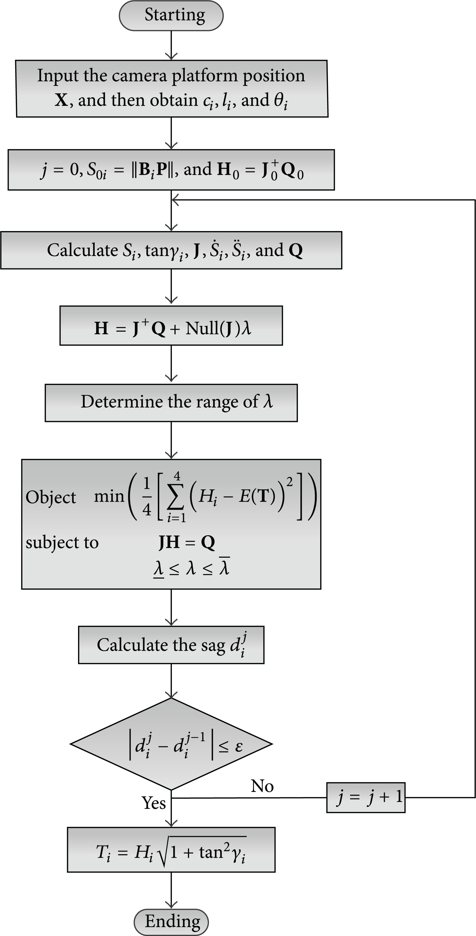
In order to ensure the normal work of the camera robot, the tension T_i must meet the following condition:

T_{\min} \leq T_{i} \leq T_{\max},

(18)

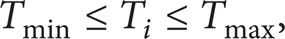
where the lower bound of the cable tension T_min is required to keep cables taut, whereas upper bound of the cable tension T_max is limited by the output torques of the servomotors and the maximum tension of the cable can withstand without breaking.

Substituting (13)–(17) into (18) yields the following expression:

λ_{i}^{t} \in R_{i}^{t} (i = 1,2, 3,4),

(19)

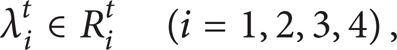
where λ_i^t is the range of λ satisfying (18). Since the camera robot has four cables, (20) consists of four expressions. Hence, the range of λ is expressed as

λ^{T} = R_{1}^{T} \cap R_{2}^{T} \cap R_{3}^{T} \cap R_{4}^{T} .

(20)

A significant measure to ensure that the camera robot works normally is to keep the cables taut, which can be guaranteed through making the sag-to-span ratio q_i meet the following condition:

q_{i} = \frac{| d_{i} |}{l_{i}} \times 100 % \leq 10 % .

(21)

Substituting (3) and (13)–(17) into (21), the range of λ is expressed as

λ^{d} \in R_{i}^{d},

(22)

where λ_i^d is the range of λ meeting (21). Similar to (20), (22) also comprises four expressions. Hence, the range of λ is expressed as

λ^{d} = R_{1}^{d} \cap R_{2}^{d} \cap R_{3}^{d} \cap R_{4}^{d} .

(23)

Combining (20) and (23) gives the following expression:

λ = λ^{T} \cap λ^{d} = [\underline{λ}, \bar{λ}],

(24)

where $\underline{λ}$ is the lower bound of λ; $\bar{λ}$ is the upper bound.

4.3. Optimal Model of the Cable Tension Distribution

It can be known from (15) that the homogeneous solution H _h is infinite due to the arbitrariness of λ. The problem of finding a unique solution to cable tension distribution among the four cables can be dealt with by using optimizations [3 –6, 18, 20].

For the stable operation of the camera robot, a severe deviation must be avoided. Thereby, a reasonable cable tension distribution is to make the tension deviations as small as possible. Consequently, the stable operation of the camera robot may be anticipated. Thus, the minimum variance can be used as the optimal object. If (12) and (24) are the constraint conditions, the optimization comes out a constrained optimization. Mathematically, the optimal model of the constrained optimization can be expressed as follows:

\begin{matrix} Object f (λ) = \min_{} (\frac{1}{4} [\sum_{i = 1}^{4} {(H_{i} - E (H))}^{2}]) \\ subject to J H = Q \\ \underline{λ} \leq λ \leq \bar{λ}, \end{matrix}

(25)

where H_i = H_sⁱ + Nλ, E( H ) = (∑_{i = 1}⁴(H_sⁱ + N_iλ))/4. Substituting (13)–(17) into (25) leads to a second-order polynomial in terms of a single variable λ as follows:

F (λ) = α_{1} λ^{2} + α_{2} λ + α_{3},

(26)

where α₁, α₂, and α₃ depend on H_i and N_i. The optimal solution λ* can be figured out with the following 3 types:

\begin{matrix} (Ι) r_{i}^{*} \geq \bar{λ}, λ^{*} = \bar{λ}, \\ (Ι Ι) \underline{λ} < r_{i}^{*} < \bar{λ}, λ^{*} = r_{i}^{*}, \\ (Ι Ι Ι) r_{i}^{*} \leq \underline{λ}, λ^{*} = \underline{λ}, \end{matrix}

(27)

where r_i* = − α₂/2α₁ [20].

5. An Iterative Optimization Algorithm of the Cable Tension Distribution

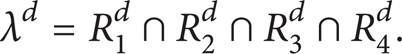
Equation (12) is a highly nonlinear equation. In order to solve the nonlinear equation, we introduce an iterative optimization algorithm to solve the cable tensions. It is well known that the initial iterative values have a significant impact on the iterative method. After several trails, we use the cable tensions and lengths obtained by massless straight line model as the initial ones. Thus, the iterative optimization algorithm of tension distribution can be summarized as follows.

Input the camera platform position X in the workspace, and obtain l_i, c_i, and θ_i.

Calculate the initial length S_0i = ∥ B _i P ∥ of cable i, which is the chord length, input the linear cable density ρ, and then calculate ${\dot{S}}_{0 i}$ , ${\ddot{S}}_{0 i}$ , and Q ₀.

Calculate the initial value $\tan γ_{0 i} = \frac{c_{i}}{l_{i}}$ at the cable end node P of every cable; the initial value $J_{0} = {[J_{01} J_{02} J_{03} J_{04}]}^{T}$ of J , in which $J_{0 i} = {[\cos θ_{i} \cos θ_{i} \tan γ_{0 i}]}^{T}$ . Calculate the initial value H ₀ = J ₀⁺ Q ₀ of H .

Obtain the range of λ due to (18)–(24).

Calculate H = J ⁺ Q + N ( J )λ according to (13).

Calculate d_i according to (3).

Update the new value of S_i, $\tan γ_{i} = d z_{i}^{s} / {d x_{i}^{s} |}_{x_{i}^{s} = l_{i}} = - \sinh {((2 β_{i} x_{i}^{s} / l_{i}) - α_{i}) |}_{x_{i}^{s} = l_{i}}$ , J , ${\dot{S}}_{i}$ , ${\ddot{S}}_{i}$ , and Q .

Judge whether the condition |d_i^j − d_i^{j − 1}| ≤ ε (ε is the iterative stop threshold) is satisfied or not. If it is, stop the iterative process. If it is not, go to (e), and repeat the process from (e)–(h), j = j + 1.

Calculate T_i according to (17).

The flowchart of the cable tension iterative optimization algorithm is shown in Figure 6.

Figure 6:

Flowchart of the cable tension iterative optimization algorithm.

6. Numerical Examples

6.1. Convergence and Effectiveness of the Algorithm

This example is used to verify the good convergence and effectiveness. The parameters of the camera platform model used in this example are listed in Table 1.

Table 1:

Parameters of the camera robot model.

System parameters	Symbol	Value

Linear density of the cable	ρ	0.188 kg/m
Discrete node number of each cable	η	60
Mass of the camera platform	m _p	50 kg
Lower bound of the cable tension	T _min	55 N
Upper bound of the cable tension	T _max	4000 N
Iterative stop threshold	ε	0.01 m
Position of 1# pulley (see Figure 1)	B ₁	(0,0,50)^T m
Position of 2# pulley	B ₂	(100,0,50)^T m
Position of 3# pulley	B ₃	(100,80,50)^T m
Position of 4# pulley	B ₄	(0,80,50)^T m

Seeing Figures 7 and 8, suppose that the motion trajectory is a spatial spiral described as follows:

\begin{matrix} x = R \cos (ω t) + 50, \\ y = R \sin (ω t) + 50, \\ z = v t + 10, \end{matrix}

(28)

where R = 20 m; ω = 0.2π rad/s; v = 1.5 m/s. t = 0: Δt: t_dur is a series of discrete time points; the duration time of the entire trajectory t_dur = 10 s; the discrete time step Δt = 0.1 s. The starting position of the trajectory is (70, 50, 10)^T m; the ending position of the trajectory is (70, 50, 25)^T m.

Figure 7:

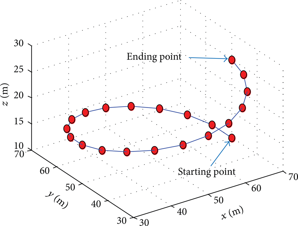
Spiral trajectory of the camera platform.

Figure 8:

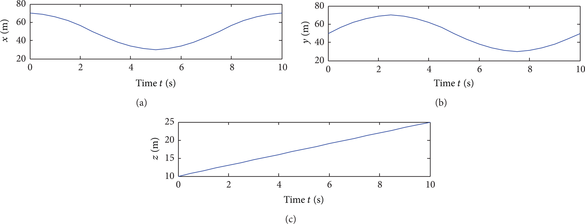
Spiral trajectory description in x-, y-, and z-component.

Figure 9(a) depicts the iterative number in every point of the trajectory. The maximum iterative number is 5, which confirms the good convergence of the algorithm presented in this paper. It also verifies the rationality selection of the initial iterative. Figure 9(b) shows the continuous variation of λ*, which is the optimal value of λ in every point. The trajectory is continuous, so λ* varies continuously.

Figure 9:

Iterative number and λ* in every point along the trajectory using the iterative optimization algorithm.

In order to verify the validity of the iterative optimization algorithm, we compute the variances under two conditions: one is the variance of the special solutions to the tensions (excluding the optimization algorithm); the other is the variance of the tensions (including the optimization algorithm). As shown in Figure 10, variances of the tensions including optimization algorithm are obviously smaller than those excluding the optimization algorithm.

Figure 10:

Variances excluding and including the optimization algorithm along the trajectory.

As Figures 11(a) and 11(b) illustrate, the cable lengths and tensions vary continuously. Due to (28), the height of the camera platform at the ending point rises by 15 m from the starting point. Thus, the lengths of the four cables at the ending point are all shorter than those at the starting point. Nevertheless, the angles between the tensions T_i and their vertical components V_i increase with the height rising of the camera platform, so the tensions must increase to withstand the weights and inertias of the cables and camera platform. Consequently, the tensions of the four cables at the ending point are larger than those at the starting point. The results verify the reasonability of the algorithm.

Figure 11:

Cable lengths and tensions of four cables along the trajectory with the iterative optimization algorithm.

6.2. Necessity of Considering the Cable Sags and Inertias

In order to show the necessity of taking the cable sags and inertias into account, we compute the tensions using the catenary and massless straight line model, respectively. The maximal relative difference of tensions can be used for assessing the divergences between the two models [15], which can be expressed as follows:

χ_{i} = \max_{i = 1,2, 3,4} (\frac{T_{i} - T_{i}^{'}}{T_{i}^{'}} \times 100 %),

(29)

where T_i is the tension in the cable i at cable end P obtained with the catenary model and T_i′ is the tension in cable i obtained by the massless straight line model. In order to study the maximal relative difference in detail, we compute it across z-direction horizontal workspace sections in three cases: the large-dimensional one, medium-dimensional one, and small-dimensional one. The camera platform has an acceleration of (0, 0, 2) m/s² at every point across the three workspace sections; other system parameters are listed in Table 1. The fixed pulleys positions of these three cases are listed in Table 2. The results are plotted in three nephograms as shown in Figures 12(a)–12(c).

Table 2:

Positions of the fixed pulleys for the three cases.

Positions of the fixed pulleys	Symbol	Case 1	Case 2	Case 3

Position of 1# pulley (see Figure 1)	B ₁	(0, 0, 50)^T m	(0, 0, 25)^T m	(0, 0, 3)^T m
Position of 2# pulley	B ₂	(100, 0, 50)^T m	(50, 0, 25)^T m	(5, 0, 3)^T m
Position of 3# pulley	B ₃	(100, 80, 50)^T m	(50, 40, 25)^T m	(5, 4, 3)^T m
Position of 4# pulley	B ₄	(0, 80, 50)^T m	(0, 40, 25)^T m	(0, 4, 3)^T m

Figure 12:

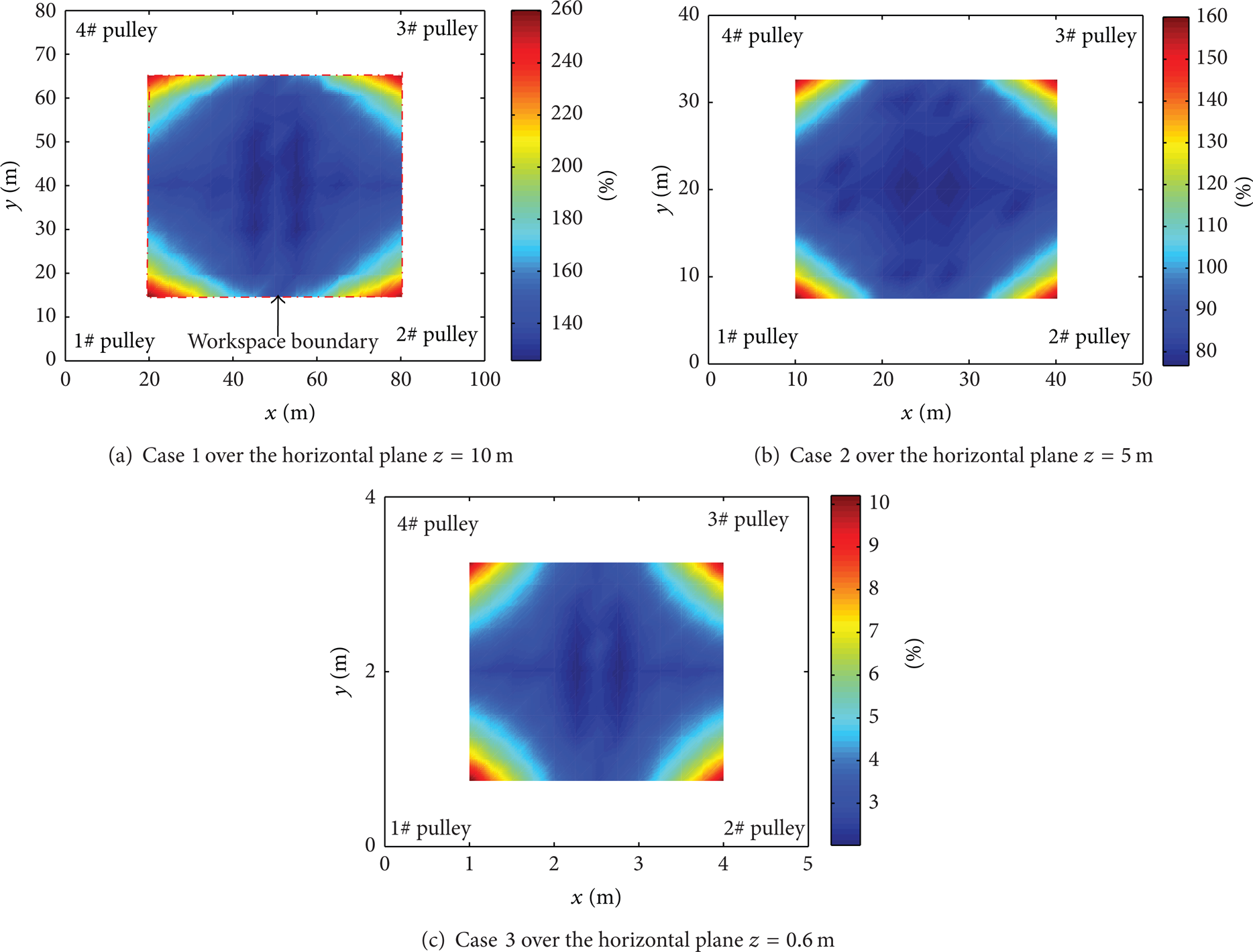
Maximal relative differences (%) on the cable tensions over the z-direction horizontal workspace sections (catenary model versus massless straight line model).

Figure 12(a) shows the obvious relative differences on all cables across the plane z = 10 m, and the maximal relative differences of four cables are about 260%. This demonstrates that taking the cable sags and inertias into account for the large-dimensional case is very necessary.

Figure 12(b) illustrates the big relative differences on all cables across the plane z = 5 m, and the maximal relative differences of four cables are about 160%. It is necessary to take the cable sags and inertias into consideration in the medium-dimensional case.

Figure 12(c) depicts the slight relative differences on all cables across the plane z = 0.6 m, and the maximal relative differences of four cables are 10%. Thus, the cable sags and inertias can be ignored in small-dimensional case. Straight line model can be employed for determining OCTD instead of the catenary model.

Note that all the three figures demonstrate a same phenomenal; namely, the values of χ_i are relatively large in the four corners but small in the central areas of the planes. The farther the areas away from the center of the workspace planes, the bigger the values of χ_i. It means that the cable is prone to slack in these areas; it also indicates that the divergences between the two models are relatively small in the central areas. At corner areas, the lengths of the cables are longer than those at other areas, so the weighs of the cables are greater than those at other areas. As a result, the tensions at the corner areas get larger than those at the central areas.

As for the small-dimensional case, the maximal relative differences are slight. Consequently, we can use the straight line model instead of the catenary model. But for the medium- and large-dimensional cases, the relative differences are rather great. Thus, ignoring the influence of the cable sags and inertias will yield relatively serious errors. For the force or force/position control, it is very possible to deviate from the desired forces or positions. Consequently, it is very necessary to take the cable sags and inertias into consideration when the sizes of the manipulators are large.

6.3. Sag-to-Span Ratio Characteristics

We also analyze the characteristics of sag-to-span ratio in the workspace. The parameters are the same as the ones of Case 1 in Section 6.2. Figure 13 draws the sag-to-span ratio of cable 2 across the horizontal plane z = 10 m; yet, due to the symmetry, it is easy to obtain the similar sag-to-span ratios across the plane z = 10 m of cables 1, 3, and 4. The maximum value of sag-to-span ratio is about 7%, which is less than 10%. The result verifies the ability of limiting the sag-to-span ratio of the algorithm.

Figure 13:

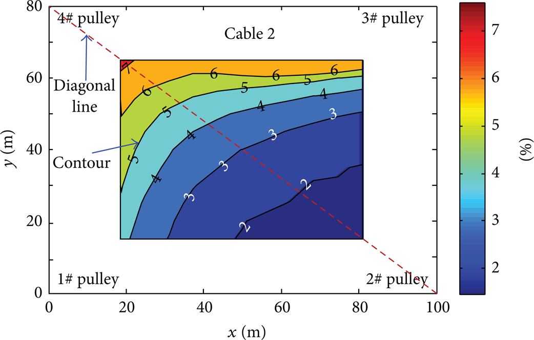
Sag-to-span ratio of cable 2 over the plane z = 10 m for a 50 kg camera platform (Case 1, the large-dimensional case).

We can see an obvious tendency; that is, the farther the distance from the 2# pulley, the larger the sag-to-span ratio. This finding agrees well with the common practice. The reason of this phenomenal is that the self-weight of the cable increases with the elongation of the cable length, leading to the radial increase of the sags. The contours in this figure denote the identical sag-to-span ratios in the workspace plane. The contours seem to be the curves, whose centers of the curves are at 2# pulley. The cable 2 is the longest along the diagonal line from 2# pulley to 4# pulley, so the contours protrude to 4# pulley. It is obvious that the sag-to-span ratio is the largest at the upper left corner of the workspace; it also means that the divergence between the catenary and straight line is the largest at this point, which fits well with Figure 12.

7. Conclusions

The camera robot is a large-span redundantly parallel cable-driven manipulator with high maneuverability. As a consequence, the dynamic model of the camera robot must include both cable sags and inertias. In order to compute the inertias of the cables, the fast length-varying catenary cables are discretized. Then, the dynamic model of the camera robot combined with the cable sags and inertias can be established which, to the best of our knowledge, has never been applied to high-speed redundantly parallel cable-driven camera robots. Furthermore, this kind of dynamic modeling can be applicable to other large-span parallel cable-driven manipulators with high-speed motions.

By using the proposed dynamic equation and sag-to-span ratio as the constraint conditions, we establish the optimal model for the cable tension distribution among the four cables. Based on the optimal model, an iterative optimization algorithm is introduced to determine the unique solution to cable tension distribution among the infinite solutions.

The simulation results show that the algorithm offers the validity, reasonability, and good convergence. The three nephograms (Figures 12(a)–12(c)) depict the three different tension maximal relative differences in the three cases. It can be concluded by analysis that the cable sags and inertias can be neglected for the small-dimensional cable-driven manipulators, but the cable sags and inertias must be taken into consideration for the medium- and large-dimensional ones. The contour map (Figure 13) illustrates the ability to limit sag-to-span ratio of the algorithm and distribution regularity of the sag-to-span ratio.

Conflict of Interests

The authors declare that there is no conflict of interests regarding the publication of this paper.

Footnotes

Acknowledgment

The authors gratefully acknowledge the financial support of National Natural Science Foundation of China under Grants nos. 51175397 and 51105290.

References

Vincent

T. L.

, “Applications of control—stabilization for film and broadcast cameras,” IEEE Control Systems Magazine, vol. 28, no. 1, pp. 20–25, 2008.

spidercam, “Technical,” 2013, http://www.spidercam.org/en/technical.

Hassan

and Khajepour

, “Optimization of actuator forces in cable-based parallel manipulators using convex analysis,” IEEE Transactions on Robotics, vol. 24, no. 3, pp. 736–740, 2008.

Pott

Bruckmann

, and Mikelsons

, “Closed-form force distribution for parallel wire robots,” in Computational Kinematics, pp. 25–34, Springer, Berlin, Germany, 2009.

Borgstrom

P. H.

Jordan

B. L.

Sukhatme

G. S.

Batalin

M. A.

, and Kaiser

W. J.

, “Rapid computation of optimally safe tension distributions for parallel cable-driven robots,” IEEE Transactions on Robotics, vol. 25, no. 6, pp. 1271–1281, 2009.

Gosselin

and Grenier

, “On the determination of the force distribution in overconstrained cable-driven parallel mechanisms,” Meccanica, vol. 46, no. 1, pp. 3–15, 2011.

Riehl

Gouttefarde

Krut

Baradat

, and Pierrot

, “Effects of non-negligible cable mass on the static behavior of large workspace cable-driven parallel mechanisms,” in Proceedings of the IEEE International Conference on Robotics and Automation (ICRA '09), pp. 2193–2198, May 2009.

Kozak

Zhou

, and Wang

, “Static analysis of cable-driven manipulators with non-negligible cable mass,” IEEE Transactions on Robotics, vol. 22, no. 3, pp. 425–433, 2006.

Riehl

Gouttefarde

Pierrot

, and Baradat

, “On the static workspace of large dimension cable-suspended robots with non negligible cable mass,” in ASME International Design Engineering Technical Conferences and Computers and Information in Engineering Conference (IDETC/CIE '10), pp. 261–270, Montreal, Canada, August 2010.

10.

Bao

Duan

, and Cui

, “Jacobian analysis of a long-span cable-driven manipulator and its application to forward solution,” Mechanism and Machine Theory, vol. 45, no. 9, pp. 1227–1238, 2010.

11.

Duan

, and Bao

, “Static stiffness of a cable-supporting system with the cable sag effects considered,” Journal of Mechanical Engineering, vol. 46, no. 17, pp. 29–34, 2010.

12.

Ottaviano

and Castelli

, “A study on the effects of cable mass and elasticity in cable-based parallel manipulators,” in ROMANSY 18 Robot Design, Dynamics and Control, pp. 149–156, Springer, Vienna, Austria, 2010.

13.

Zhu

Z.-C.

, and Du

J.-L.

, “Analysis and control of the cable-supporting system including actuator dynamics,” Control Engineering Practice, vol. 19, no. 5, pp. 491–501, 2011.

14.

Yao

Tang

Wang

, and Huang

, “Dimensional optimization design of the four-cable-driven parallel manipulator in fast,” IEEE/ASME Transactions on Mechatronics, vol. 15, no. 6, pp. 932–941, 2010.

15.

Gouttefarde

Collard

J-F.

Riehl

, “Simplified static analysis of large-dimension parallel cable-driven robots,” in IEEE International Conference on Robotics and Automation River Centre, pp. 2299–2305, Saint Paul, Minn, USA, May 2012.

16.

J. L.

Wen

, and Bao

, “Cable vibration analysis for large workspace cable-driven parallel manipulators,” in Cable-Driven Parallel Robots, pp. 437–449, Springer, Berlin, Germany, 2013.

17.

Bao

Cui

, and Yang

, “Dynamic analysis of cable-driven parallel manipulators with time-varying cable lengths,” Finite Elements in Analysis and Design, vol. 48, no. 1, pp. 1392–1399, 2012.

18.

Verhoeven

, Analysis of the workspace of tendon-based stewart platforms [Ph.D. dissertation], University of Duisburg-Essen, Duisburg, Germany, 2004.

19.

Irivne

H. M.

, Cable Structures, MIT Press, Cambridge, Mass, USA, 1981.

20.

Liu

, On the mechanism performance analysis and motion control of the two types of parallel manipulators [Ph.D. dissertation], Xidian University, 2009.

Optimal Cable Tension Distribution of the High-Speed Redundant Driven Camera Robots Considering Cable Sag and Inertia Effects

Abstract

1. Introduction

2. Description

2.1. Description of the Camera Robots

2.2. Catenary Equation of the Cable

3. Dynamics of the Camera Robot

3.1. Dynamics of a Fast Varying-Length Cable

3.2. Dynamic Equation of the Camera Robot

4. Optimal Model of the Cable Tension Distribution

4.1. Cable Tension Distribution Equation

4.2. Constrained Conditions of the Optimization Model

4.3. Optimal Model of the Cable Tension Distribution

5. An Iterative Optimization Algorithm of the Cable Tension Distribution

6. Numerical Examples

6.1. Convergence and Effectiveness of the Algorithm

6.2. Necessity of Considering the Cable Sags and Inertias

6.3. Sag-to-Span Ratio Characteristics

7. Conclusions

Conflict of Interests

Footnotes

Acknowledgment

References