
Abstract
Global sensitivity is used to quantify the influence of uncertain model inputs on the output variability of static models in general. However, very few approaches can be applied for the sensitivity analysis of long-term degeneracy models, as far as time-dependent reliability is concerned. The reason is that the static sensitivity may not reflect the completed sensitivity during the entire life circle. This paper presents time-dependent global sensitivity analysis for long-term degeneracy models based on polynomial chaos expansion (PCE). Sobol’ indices are employed as the time-dependent global sensitivity since they provide accurate information on the selected uncertain inputs. In order to compute Sobol’ indices more efficiently, this paper proposes a moving least squares (MLS) method to obtain the time-dependent PCE coefficients with acceptable simulation effort. Then Sobol’ indices can be calculated analytically as a postprocessing of the time-dependent PCE coefficients with almost no additional cost. A test case is used to show how to conduct the proposed method, then this approach is applied to an engineering case, and the time-dependent global sensitivity is obtained for the long-term degeneracy mechanism model.
1. Introduction
Nowadays, with the development of the computer science, simulation models (such as fluid dynamics (CFD) models, structural mechanics models, and kinematics models) play an important role in the areas of uncertainty quantification (UQ), reliability analysis (RA), and reliability-based design optimization (RBDO). In order to obtain the accurate estimate of the uncertainty of model output, we have to run a great number of model simulations. Consequently, the simulation burden is intractable especially for long-term degeneracy model. Sensitivity analysis (SA) helps to quantify the relative importance of each input parameter [1]. Thus, the parameters that are less important may be treated as deterministic in RA or constant in RBDO. That means the model can be simplified and the simulation burden will also be greatly reduced. As a result, both RA and RBDO can benefit from the SA.
Methods of SA are usually classified into two categories: local SA and global SA [2]. The former focuses on how little variations of the inputs in the vicinity of given values influence the model response. The latter is related with quantifying the output uncertainty due to changes of the input parameters (which is taken singly or in combination with others) over their entire domain of variation [3]. Comparing to local SA, global SA is superior when considering cases where the assumption of linearity is invalid [4]. Besides, it evaluates the effect of a factor while all other factors are varied as well and thus it accounts for interactions between variables and does not depend on the choice of a nominal point [5, 6].
In the last decade, numerous endeavors have been made to develop the global SA methods, such as Fourier amplitude sensitivity test (FAST), Morris method, and Sobol’ method. Among all the global SA methods, this paper is interested in the Sobol’ method because the Sobol’ indices provide a clear and accurate indication on the selected uncertain parameters [7] and have been shown to be robust [8]. However, the Sobol’ sensitivity indices are always calculated using crude Monte Carlo simulation. The computation cost is unacceptable when the demanding model is complex. Thus, these indices are hardly applicable for engineering practice [9].
In order to overcome the above issues, some papers proposed to conduct global SA using a surrogate model called polynomial chaos expansion (PCE) in recent years. The surrogate model can approximate the computational simulation model analytically with acceptable numerical error. Then, the Sobol’ indices can be obtained straightforward through the PCE. Sudret [7] proposed generalized PCE to build a surrogate model which allows to compute the Sobol’ indices analytically as a postprocessing of the PCE coefficients. Crestaux et al. [10] used PCE for SA and proposed that the PC-based method has some disadvantages in large dimensional problems because the number of coefficients to be computed grows dramatically with the size of the input random vector. To circumvent this problem, Blatman and Sudret [3] proposed the sparse PCE to compute Sobol’ indices; this method can handle the problem with high dimensions well. Formaggia et al. [11] conducted UQ for a basin-scale geochemical compaction model. The method is based on sparse grid sampling techniques in the context of a generalized PCE.
In recent decades, many studies have been devoted to the time-dependent RA [12] and time-dependent RBDO [13–15]. The inputs (such as design parameters, loads, and material properties) of the degeneracy model vary with time, so the interested output is time-dependent consequently. To deal with the time issue, time-dependent RA and time-dependent RBDO are extremely time-consuming. As mentioned, global SA is an effective tool for static RA or RBDO since the simulation effort can be greatly reduced according to the ranking of sensitivity indices. However, the global sensitivity indices at the initial instant cannot reflect the completed sensitivity during the product life cycle. In this case, time-dependent global SA is necessary for the long-term degeneracy model. Most literatures on the global SA concentrate on the static models, and time-dependent global SA for time-dependent RBDO is rarely investigated so far. Sandoval et al. [16] proposed the global SA for dynamic models using the method of PCE. The paper concentrates on the sensitivity function of the dynamic model during a short time, for example, 10 seconds. In order to obtain the accurate sensitivity with time, PCEs have to be generated at a very small time step, for example, 0.2 s. However, as for a long-term degeneracy model, it is not quite practical because of the unacceptable computation burden.
In order to meet the needs of time-dependent RBDO for the long-term degeneracy simulation model, this paper proposes the time-dependent global SA method, which aims at quantifying the relative importance of uncertain input variables onto the output of a long-term degeneracy system during the whole life cycle. To overcome the difficulty of generating PCEs for long-term degeneracy model, this paper proposes a MLS-based time-dependent PCE coefficients computation method. Thus, the computation burden of the time-varying Sobol’ indices can be greatly simplified.
The paper is organized as follows: long-term degeneracy simulation model for mechanical considering wear is presented in Section 2. In Sections 3 and 4, time-dependent global SA and time-dependent PCE for the model output are presented, respectively. Section 5 proposes a MLS-based time-dependent PCE coefficients computation method. Section 6 proposes a PC-based method to compute time-dependent Sobol’ indices. In Section 7, the procedure of the work is formulated. A test case and an airborne retractable case are studied, respectively, in Section 8. Conclusions are drawn in Section 9.
2. Long-Term Degeneracy Simulation Model for Mechanism Considering Wear
As mentioned in Section 1, many models can be viewed as long-term degeneracy models because of the time-variant parameters and loads. As a consequence, the interested output of model may be influenced and changed with time. For instance, as for a linkage mechanism, wear of the hinges (degradation of the parameters) would affect the kinematic stability and raise the stress in hinges (the interested output of model).
In Section 8.2, our case also uses the model considering wear, because wear is one of the most critical failures in mechanical model. Wear substantially deteriorates the kinematic reliability and structural reliability of mechanisms in their service life.
In this section, a long-term degeneracy multidiscipline simulation model that includes kinematics model, structural finite element (FE) model, and wear model is constructed.
2.1. Wear Model
As for the plastically dominated wear, Archard's law would serve as the appropriate model as discussed by Lim and Ashby [17]. According to this model, the worn out volume is considered to be proportional to the normal load.
The model is expressed mathematically as follows:

where dw/dt is defined to be the wear volume loss rate, K is the dimensionless wear coefficient, F
N
is the applied normal force,

where h is the wear depth, dh/dt is the wear rate, and P is the contact pressure. We have K H = K/H, and it is defined as the wear coefficient with the dimension of (Pa−1).
2.2. Long-Term Degeneracy Simulation Model for Mechanical Considering Wear
In Archard's wear law, the wear rate is a function of both the pressure and the relative sliding velocity of two contact surfaces. The pressure can be obtained through nonlinear FE analysis (FEA), while the relative sliding velocity requires kinematics analysis.
For a linkage mechanism, the multidiscipline simulation model considering wear includes kinematics model and structural FE model. For the sake of simplicity, this paper assumes the wear depth of each task is a constant denoted by Δh. In order to compute Δh, the kinematics model of the mechanism is constructed to obtain the relative sliding velocity v of hinges, and loads on hinges can also be given by the kinematics model. Then these loads are transmitted into the structural FE model, which is built by commercial finite element software ANSYS. FE model of hinges is solved by the nonlinear contact analysis to compute the contact pressure p. After that, the conduct pressure and sliding velocity are delivered to the wear model to calculate the wear depth Δh. The procedure to compute Δh is represented in Figure 1.
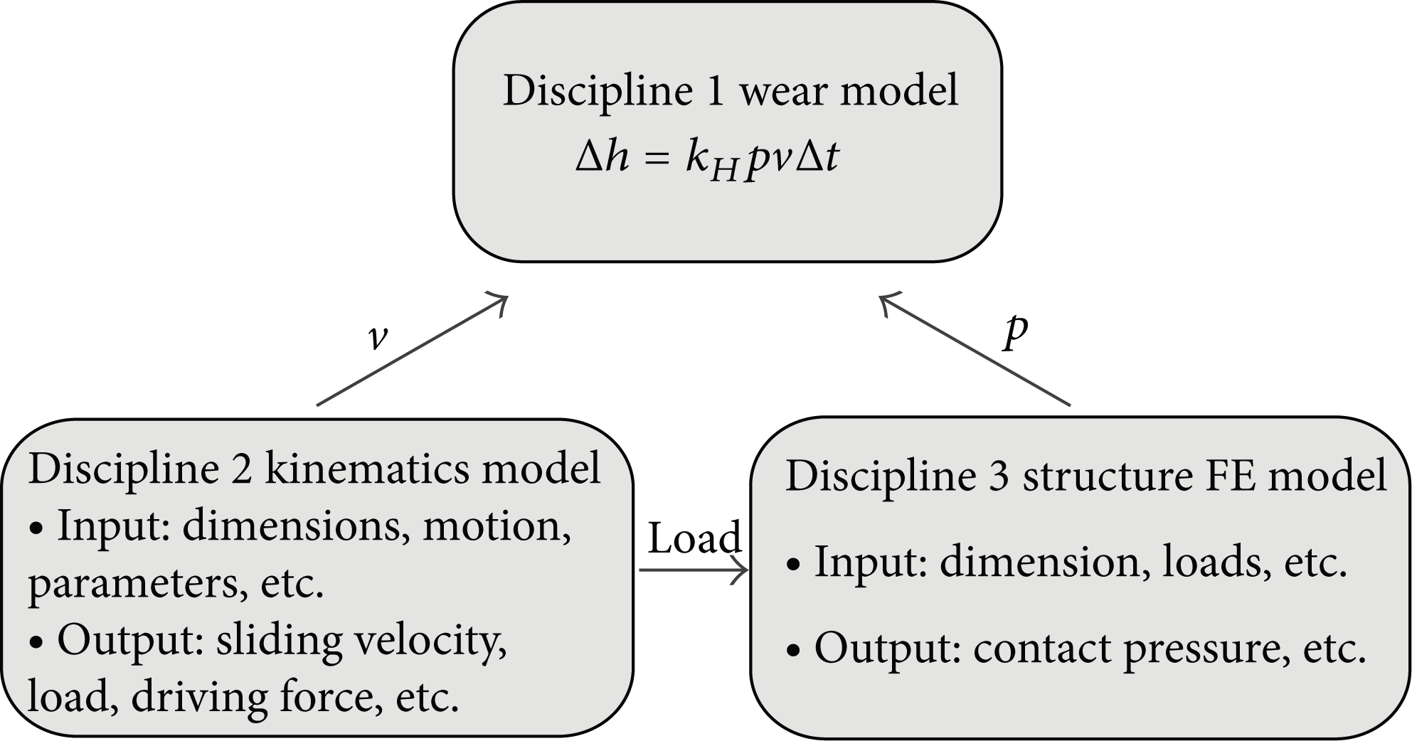
Schematic of the computation of Δh.
Thus, we can define our long-term degeneracy simulation model for mechanism considering wear as follows:

where y is the interested output,
3. Time-Dependent Global SA
As mentioned in Section 1, this paper uses the time-dependent Sobol’ indices for global SA. First, the time-dependent Sobol’ function decomposition is investigated; then the time-dependent Sobol’ indices are defined.
3.1. The Time-Dependent Sobol’ Functional Decomposition
Let us consider a time-dependent model y(t) = y(t,

The number of Ω in the right-hand side of (4) is k, according to [18]; at each time instant, the output of model y can be decomposed as follows:
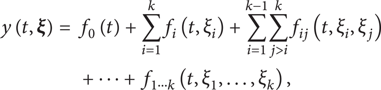
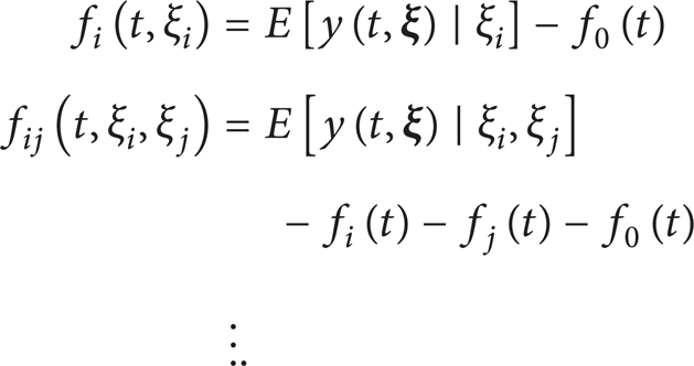
where y(t,

Besides, the integral of each summand

Thus, the summands are orthogonal to each other:

where {i1,…,i s }≠{j1,…,j m }.
From the representation above, the decomposition in (5) is unique whenever y(t,
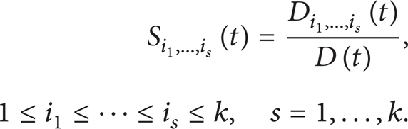
3.2. The Time-Dependent Sobol’ Sensitivity Indices
Following the above representation, the variance of y(t,
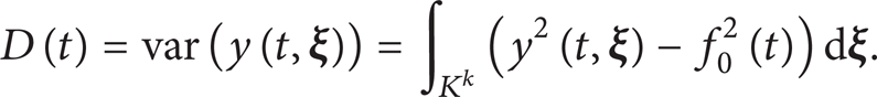
The D(t) can be derived straightforward as follows:

with

As the model is a time-dependent one, the output of the model y(t,
By definition, according to (11), the following expression is obtained:

Each
The total sensitivity function of parameter ξ i is defined by

which accounts for the total contribution to the output variation due to the parameter ξ i at each time instant.
However, the Sobol’ indices are practically computed using Monte Carlo simulation, which makes them hardly applicable for computational simulation models [7], especially as they are required to perform at each time instant. To solve this problem, a surrogate model called time-dependent PCE used to represent the response of the long-term degeneracy model is invested. The next section will introduce the time-dependent PCE in detail.
4. Time-Dependent PCE for the Model Output
Polynomial chaos expansion is a promising surrogate model that uses a set of orthogonal polynomial basis to approximate the random space of the system response [19]. There are two types of PCE methods: intrusion approach and nonintrusive approach according to the method to compute the coefficients of PCE. Intrusion approach is difficult, expensive, and time consuming for many complex computational problems [20]. Thus, this paper employs nonintrusive method to compute the coefficients of PCE.
The polynomial chaos for a dynamic system response can be described as follows [21–23]:

where r(t,

where

where

where n is the number of random variables in the system.
The multidimensional Hermite polynomials form an orthogonal basis for the space of square-integrable PDFs, and the PCE is convergent in the mean square sense [25]. In general, the approximation accuracy rises with the order of the PCE. Except for Hermite polynomials, one can also use other orthogonal polynomials from the generalized Askey scheme for some standard non-Gaussian input uncertainty distributions, for example, Laguerre polynomials for gamma distributions, Jacobi polynomials for beta distribution, and Charlier polynomials for Poisson distribution, and so forth [19]. For any arbitrary input distribution, a Gram-Schmidt orthogonalization can be employed to generate the orthogonal family of polynomials [26].
If the distribution types of each parameter are not unified, we have to represent all uncertain parameters in terms of a set of standardized random variables (SRVs), in order to get an orthogonal basis for the related polynomials. This paper suggests mapping the different distribution random variables onto the standardized normal random variable. The transformation functions are given in Table 1. The reason is that they have been extensively studied and their functions are typically well behaved [25]. What is more, this paper derives that the standardized normal random variables also have some advantages on numerical characters of statistics (see (42) in Section 6). Besides, if the input parameters are not mutually independent, a transformation process with a covariance matrix is necessary. The steps of transformation process can be seen in [25].
Transformation of common distribution of standardized normal random variables.

Once the time-dependent PCE is available, the time-dependent Sobol’ indices can be easily obtained (see Section 6). One of the critical issues for time-dependent PCE is how to estimate the time-dependent PCE coefficients efficiently. In the next section, we propose a new method to compute the time-dependent PCE coefficients. The PCE is only required to build at some selected time points; thus, the simulation cost is highly saved.
5. Computation of the Time-Dependent PCE Coefficients
As for a static model, probabilistic collocation method (PCM) is one of the most efficient methods to compute the coefficients of PCE in nonintrusive PCE method [15]. The coefficients of the PCE are obtained according to evaluations of the system responses at selected collocation points, and these collocation points correspond to the roots of the polynomial of one degree higher than the order of the PCE [20]. Furthermore, the probabilistic collocation method just requires calls of the simulation the same as the number of PCE coefficients; thus, it is very efficient.
However, collocation methods are inherently unstable, especially with PCE of high order [25]. Thus, the paper proposes an extensive probabilistic collocation method based on regression, which needs to select a number of points equaling twice the number of coefficients. The case in the paper indicates that the estimation of the coefficients of PCE through this method is more robust than the collocation method.
This paper proposes an algorithm which is based on the extension of PCM and moving least squares (MLS) to compute the time-dependent PCE coefficients. In this section, we start by recalling the extension of PCM method to obtain the estimation of the PCE coefficients and the MLS method. Then, we introduce our algorithm to calculate the time-dependent PCE coefficients.
5.1. The Extension of PCM Method
The extension of PCM method is a regression-based method which uses regression in conjunction with an improved input sampling method to simulate the response of the model. The collocation points are selected based on an improvement of the standard orthogonal collocation method of [27]. The rule of selecting the points is that each value of standard normal random variable ξ i has two choices, zero or the roots of the higher order Hermite polynomial. The concrete sampling scheme of this method can be found in [25].
The matrix form of the extension of PCM method is described as follows:

where
As a linear algebraic equation, if the condition number of

5.2. Moving Least Squares
MLS is a generalization of the least squares technique, and it has become a widespread and powerful tool in interpolating and approximating implicit surfaces [28–30]. MLS starts with a weighted least squares formulation for an arbitrary fixed point in R
d
, and then this point moves over the entire parameter domain, where a weighted least squares fit is computed and evaluated for each point individually. Suppose a compact set Ω⊆R
d
is given and a continuous function f will be reconstructed from its values f(x1),f(x2),…,f(x
N
) on scattered pairwise distinct centers

where d represents the dimension of the function f,q represents the order of
The weighting function is nonnegative, (∥x − x i ∥) > 0, inside the support domain Ω.
The weighting function has compact support, w(∥x − x i ∥) > 0, outside the support domain Ω.
The weighting function should be normalized, ∫Ωw(∥x − x i ∥)dΩ = 1.
The weighting function should be monotone decrease, and the weight values should decrease with the increase of the distance from x.
The most common weighting functions are spline function, compactly supported radial basis function (CSRBF), Gaussian function, and so forth. Among these weighting functions, the spline functions are used widely because their order can be chosen to obtain high approximation accuracy. Note that the higher order of the spline functions would not necessarily perform a better approximation, and the order of the spline function is decided by the highest order of the approximated function derivative.
The approximation function can be written as

where

It is defined as

where
and

where

Therefore, the approximation function can be derived as
where
5.3. MLS-Based Time-Dependent Coefficients Computation
The long-term degeneracy simulation model is simulated step by step, and one step is defined as a task execution in which the mechanism would perform a required function. The PCE is constructed on system responses at some selected steps along the service life. After this, MLS method is employed to estimate the time-dependent functions of PCE coefficients. Total Ns tasks need to be completed which is decided by the length of service life and frequency of task arrival. t i is defined as the ith selected step (or task), and m is the total number of selected steps that PCEs are required to be built on. According to (22), the coefficients for all of the PCEs are solved by the following equation:

where

where
After the calculation of Λ, a new matrix
where

where
Once the time-dependent PCE is available, the next step is computing the time-dependent Sobol’ indices. The next section proposes a PC-based method to compute these indices analytically.
6. PC-Based Time-Dependent Sobol’ Indices
The sensitivity measures are the quantitative indices of the effects of each uncertain input parameter onto the response of a simulation model and their propagation through the model. Among all kinds of literatures on sensitivity measures, the Sobol’ indices [1] have been paid much attention since they provide a clear and accurate indication on the selected uncertain parameters. In [7], Sudret first established a link between PC expansion and the Sobol’ indices. Then the computation of Sobol’ indices is much more efficient than the previous method of Monte Carlo Simulation. The author proved that the computation Sobol’ indices of a surrogate PC are analytical when the input uncertain parameters are uniformly distributed in [0, 1] and the selected polynomial basis is Legendre.
Following the ideas of Sudret, we can obtain the PC-based time-dependent Sobol’ indices.
Firstly, the mean and the variance of the r(t,

Secondly, the Sobol’ decomposition of the PCE should be derived. In order to separate the different contributions, the polynomials {ψ
j
,j = 1,…,N
c
− 1} in (18) can be reordered and the Sobol’ decomposition of r(t,

where

Thirdly, PC-based time-dependent Sobol’ indices

The (j1,…,j
t
) in (40) is a given integer sequence, and the

PC-based Sobol’ indices can be computed analytically since
Besides, if the orthogonal basis for the polynomials is Hermite, this paper derives that

7. The Procedure of the Proposed Approach
Time-dependent global SA using PCE can be conducted for a three-stage strategy (see different colors of Figure 2).

Procedure of time-dependent global SA using PCE.
(A) PC Decomposition
(A1): Polynomial Type. Choose the related type of basis for the PCE according to the types of distributions of the uncertain parameters. If uncertain parameters have different types of distribution, one must represent all the inputs in terms of a set of SRVs (see Section 4).
(A2): Transformation. If the input parameters are correlated, a transformation process with a covariance matrix ∑ is necessary.
(A3): PC Degree. Set the appropriate order n for the PC. If the order used for the PCE is p = n, then p = n + 1 should also be considered for the sake of comparing the erro r t among the real value r t obtained through simulation of model, the response r t n estimated from n-order PCE, and the response r t n + 1 estimated from (n + 1)-order PCE (see Figure 2). The cyclical process helps to judge a final n as the order of PCE.
(A4): PC Truncation. Compute the number of N c − 1 summands in (18) according to (19).
(B) Time-Dependent PCE Coefficients. Compute the time-dependent PCE coefficients according to the proposed method in Section 5.3. Firstly, the PCEs are built at some selected time points, and the condition number of
(C) Time-Dependent Sobol’ Indices. Once the time-dependent PCE coefficients are available, the PC-based time-dependent Sobol’ indices can be computed analytically according to (39) to (40).
8. Case Study
8.1. Test Case
To illustrate the contribution of this paper, an ideal mass-spring-damper system is considered, with a mass m, a spring constant b, and a viscous damping coefficient k, subject to a constant force F, as represented in Figure 3. k is assumed as a degradation parameter. We assumed that the life of this system is 2000 tasks.

Mass-spring damper system.
This system can be described by the following differential equation:

where y(t) is the output of the system, which means the mass position. Figure 4 is the simulation for a task when m = 1, b = 1, and k = 4.5.
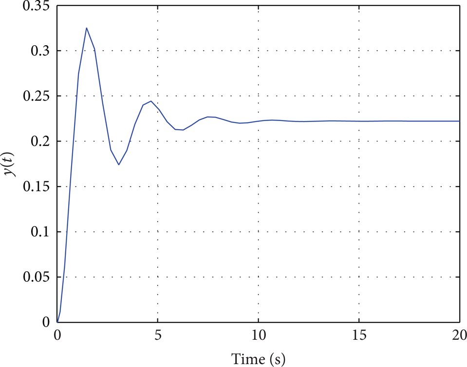
Mass position simulation.
In this case, the maximum mass position max- y in every task is the interested output of the system. The sensitivity of the uncertainty parameters m, b, and k (listed in Table 2) on the max- y is considered, where k with a decreased constant of 2.5e − 4 at each step.
List of three uncertain parameters.
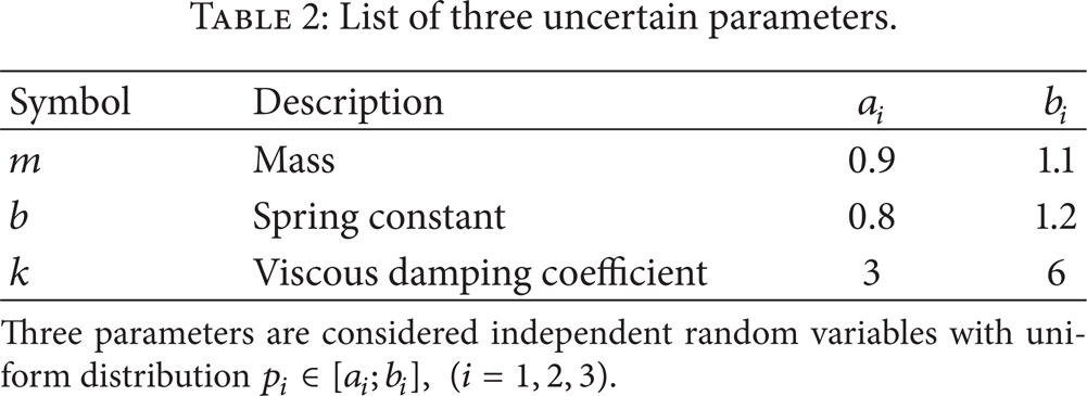
Three parameters are considered independent random variables with uniform distribution p i ∈ [a i ;b i ], (i = 1, 2, 3).
8.1.1. PC Decomposition
The selected basis of PCE is Legendre since all the three input parameters are uniformly distributed. The degree of the PCE is p = 3 which is sufficient due to the error of the response among the real value r(t) obtained through simulation of model, 2-order PCE, and 3-order PCE small enough (see Tables 3 and 4). The number of input parameters is 3; thus, the number of coefficients of 2-order PCE and 3-order PCE can be computed as n = 10 and n = 20, respectively.
Comparative results of mean of the max-y along the time axis.

Comparative results of the variance of the max-y along the time axis.

8.1.2. Time-Dependent PCE Coefficients
The sets of collocation points are selected according to Section 5.1. Then the output of the system max-y(i) in selected time points can be obtained through solving (43). The responses at every 200 steps are selected to build the PCEs, which means that the PCEs are constructed at steps 1, 200, 400, and so on till 2000. The coefficients of PCEs can be calculated by (31).
The discrete points of a0 (PCE coefficients) of the PCEs have a nearly linear increase over time. As mentioned in Section 5.2, low-order spline weighting functions should be used to approximate the functions of the PCE coefficients. In this case, the cubic spline function performs a better approximation. Thus, the cubic spline function is chosen as the weighting function which is given as follows:
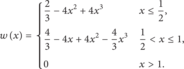
Figure 5 shows the time-varying PCE coefficient of a0. The discrete blue points are PCE coefficients calculated by PCM, and the red curve is approximated by MLS. It can be seen that the curve fits these points well. The other 14 coefficients are also built by MLS using the same method.
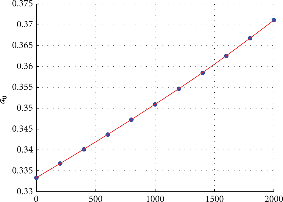
MLS approximation curve for a0 of the max-y PCE.
The comparative results of max-y are obtained at selected time steps which are 1, 500, 1000, 1500, and 2000 steps. The Monte Carlo simulation with 10000 samples is employed as a benchmark for the comparison. The statistics including the mean and the variance of the max-y are compared with the results from the 2-order and 3-order PCE. The comparison results are shown in Tables 3 and 4.
8.1.3. Time-Dependent Sobol’ Indices
Time-dependent Sobol’ indices can be computed according to (39) and (40). Figures 6, 7, 8, and 9 list the first-order, the second-order, the third-order, and the total time-dependent Sobol’ indices, respectively.

First-order time-dependent Sobol’ indices.
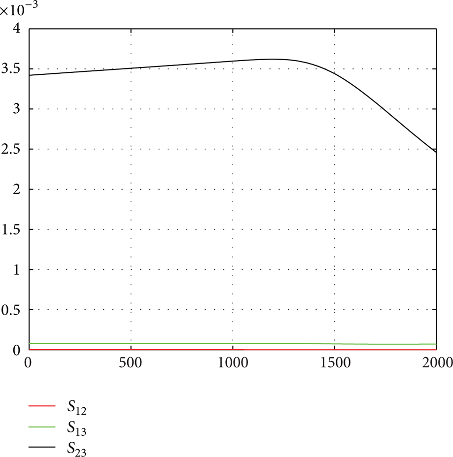
Second-order time-dependent Sobol’ indices.
Third-order time-dependent Sobol’ indices.
Total time-dependent Sobol’ indices.
It can be seen that the most influential parameter on the max- y is k obviously during the whole life cycle of the mass-spring-damper system (see Figures 6 and 9). And the higher order indices are much smaller than the first-order indices.
8.2. Engineering Case
The engineering case is an airborne retractable mechanical system (see Figure 10). It is a four-link mechanism which consists of the hydraulic actuator, rods, and pin-and-lug hinges and is designed to carry the functional device to move in accordance with the predetermined trajectory. The process that the mechanism moves from the stopping position to the working position and then moves back is defined as a task and the required consumed time is 7.2 s. Each task is a step. In the service life, the mechanism would act about 2000 times which is considered to be the total steps in the algorithm.
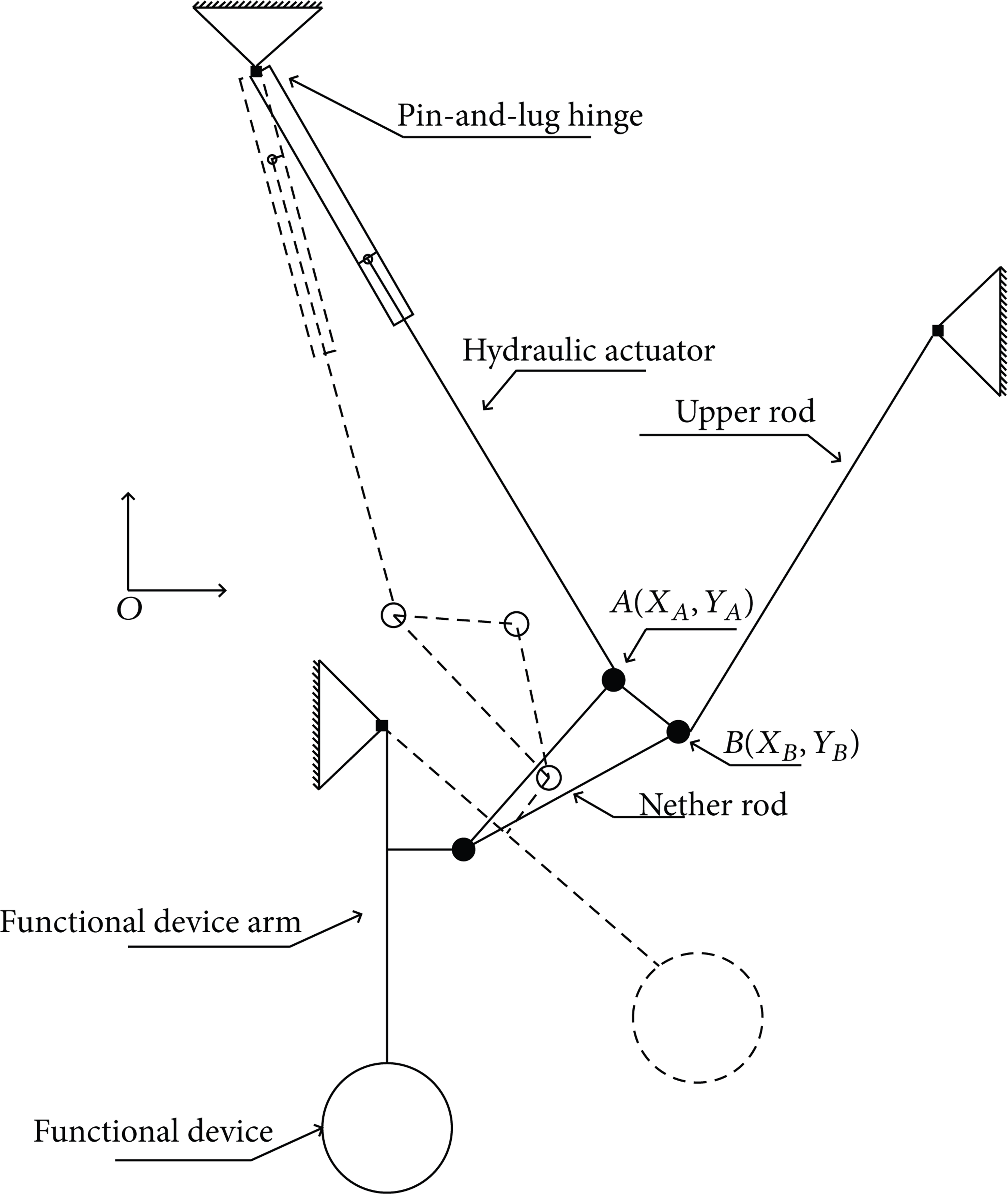
Schematic of the airborne retractable mechanical system.
At the initial design phase, the positions and orientation of the upper rod, nether rod, and hydraulic actuator are determined by requirements from higher level system. Therefore, both the lengths of the upper rod and nether rod depend on the horizontal coordinate X B and the length of the actuator depends on the horizontal coordinate X A . Thus, X A and X B are both significant design variables. When the retractable system is performing, the system is under the weight of the functional device. The top hinges are working in the nonlubricated environment. As a result, the radius of the lug Rlug is bigger and bigger for the wear of the hinges. Besides, the weight of the functional devices G d is also decreasing along time by requirements of the mechanism functions.
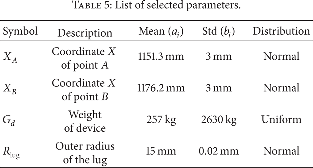
The maximum driving force, Max-Force, is the interested output of the model. The sensitivity of the uncertainty parameters X A , X B , G d , and Rlug (listed in Table 5) on the Max-Force is considered, with Rlug with an increased constant Δh and G d with a decreased constant of 2.5e − 2 (kg) at each step.
List of selected parameters.
In order to compute the wear depth Δh, the kinematics model is built by ADAMS and the FE model is built by ANSYS at the initial design point, respectively (see Section 2.2). The analysis results of two software applications are represented in Figures 11 and 12. Then the value of Δh = 1.5938 (μm) can be calculated according to Figure 1.

Driving force and instant relative velocity between pin and lug computed by the kinematics model. (a) Driving force curve during the movement; (b) instant relative velocity curve during the movement.
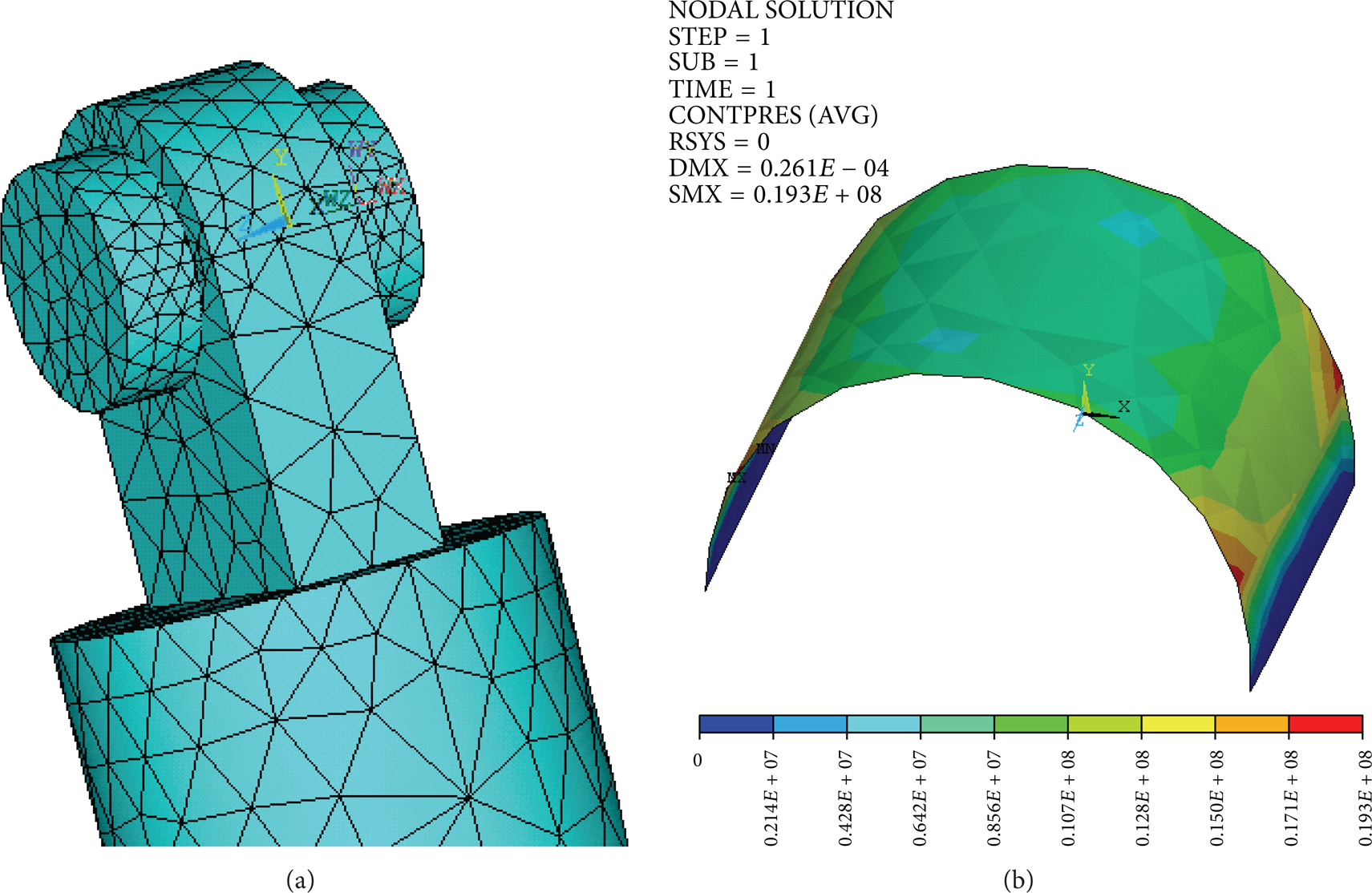
FE model and nonlinear contact analysis results exported by ANSYS. (a) FE model of the top hinge; (b) contour picture of the pressure on the contact surface of lug.
8.2.1. PC Decomposition
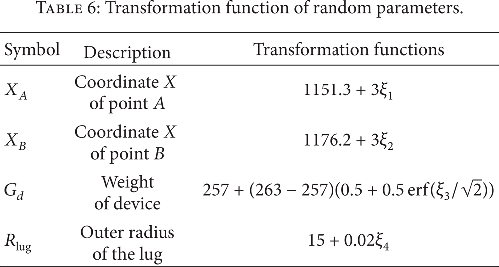
Because the four parameters have different distribution types, in order to decompose the output Max-Force in PC, the first step is transforming of inputs in terms of standard normal random variables according to Section 5.1. The transformation function can be seen in Table 6. The degree of the PCE is p = 3 which is sufficient due to the error of the response among the real value r t obtained through simulation of model, 2-order PCE, and 3-order PCE small enough (see Tables 7 and 8). The number of coefficients of 2-order PCE and 3-order PCE can be computed as n = 15 and n = 35, respectively.
Transformation function of random parameters.
Comparative results of mean of the Max-Force along the time axis.

Comparative results of the variance of the Max-Force along the time axis.

8.2.2. Time-Dependent PCE Coefficients
The sets of collocation points are selected according to Section 5.1. Then collocation points of standard normal random variables are transformed into inputs of the simulation model to get time-varying system responses, respectively. And the responses at every 200 steps are selected to build the PCEs.
After the construction of PCEs, MLS is employed to approximate the time-varying functions of PCE coefficients. Here, the cubic spline function is also chosen as the weighting function since a0 of the PCEs have a nearly linear decrease over time.
Figures 13 and 14 show the time-varying PCE coefficients of a0 and a1, respectively. The discrete blue points are PCE coefficients calculated by PCM, and the red curve is approximated by MLS. It can be seen that the curve fits these points well. The other 33 coefficients are also built by MLS using the same method.
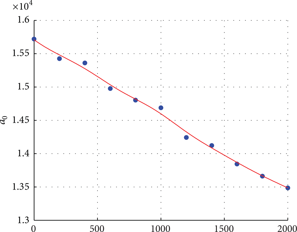
MLS approximation curve for a0 of the Max-Force.

MLS approximation curve for a1 of the Max-Force.
Then the time-dependent PCEs are constructed completely, and the time consuming simulation model is replaced by the PCEs at different time instants.
The comparative results of Max-Force are obtained at selected time steps of 1, 500, 1000, 1500, and 2000. The Monte Carlo simulation with 1000 samples is employed as a benchmark for the comparison. The statistics including the mean and the variance of the Max-Force are compared with the results from the 2-order and 3-order PCE. The comparison results are shown in Tables 7 and 8, respectively.
8.2.3. Time-Dependent Sobol’ Indices
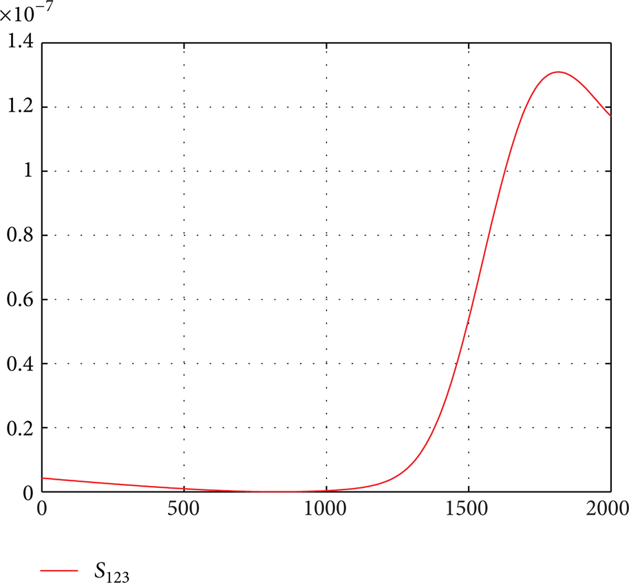
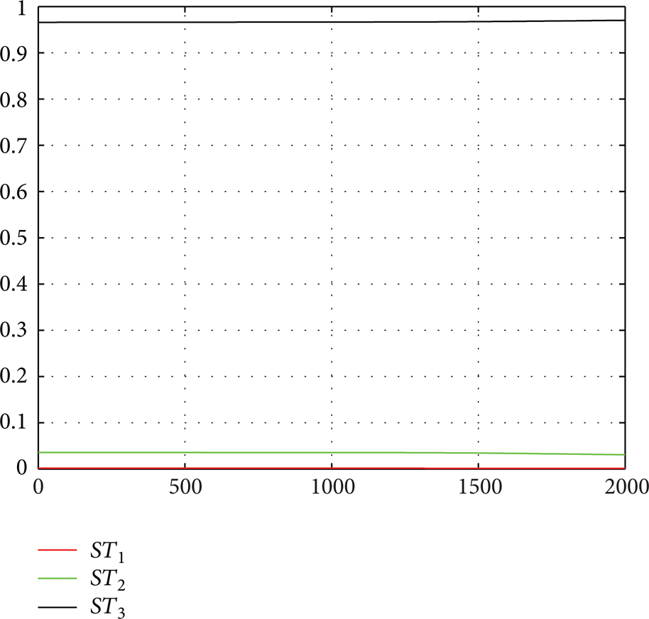
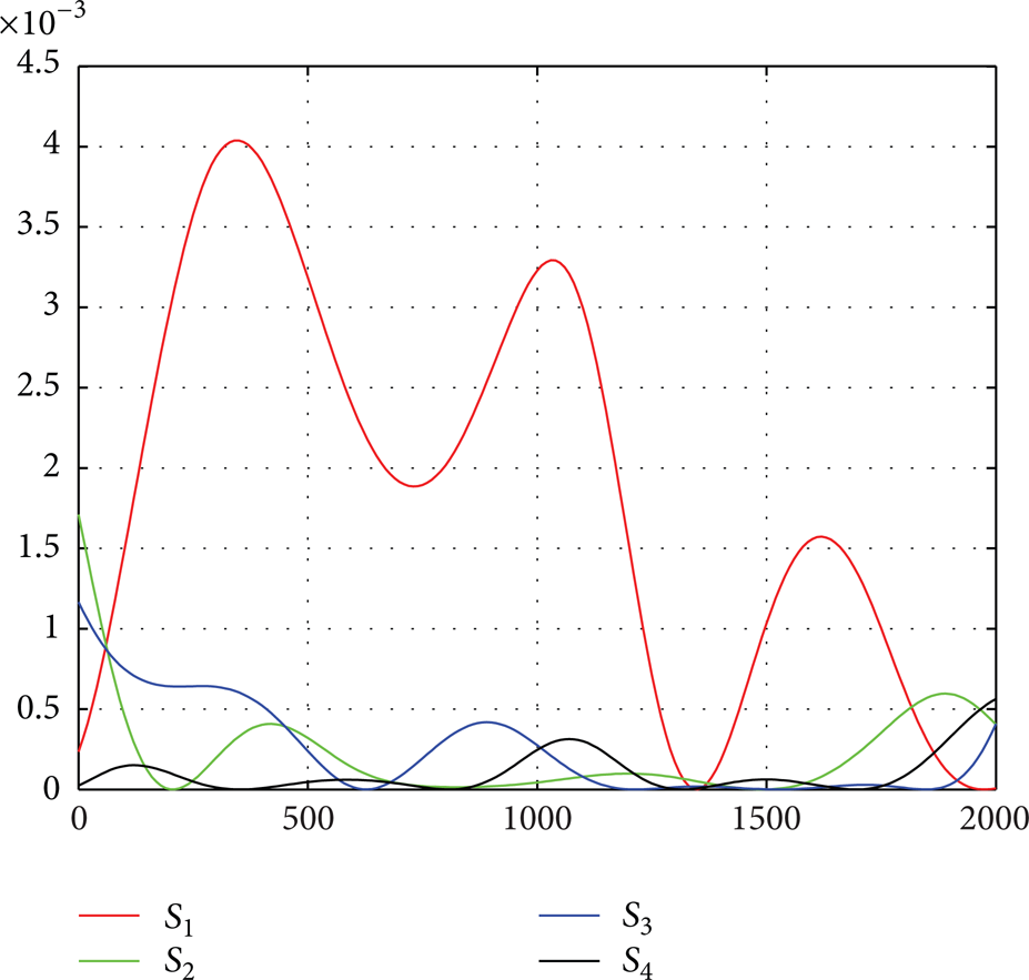
Time-dependent Sobol’ indices can be computed according to (39) and (40). Figures 15, 16, 17, and 18 list the first-order, the second-order, the third-order, and the total time-dependent Sobol’ indices, respectively.

First-order time-dependent Sobol’ indices.

Second-order time-dependent Sobol’ indices.
Third-order time-dependent Sobol’ indices.
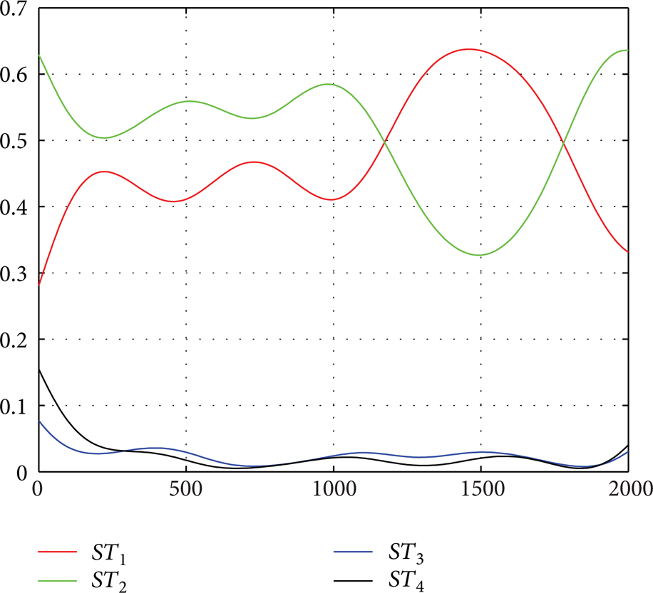
Total time-dependent Sobol’ indices.
From the representation of Figures 15 and 18, we can see that, at the initial step, the set of (X B , X A ,Rlug,G d ) is a ranking list of influential effect on the Max-Force. With the time going by, the sensitivity of four parameters is varying since the degradation of the parameters. The third-order sensitivity indices S123 (X A -X B -G d ) appear more clearly during step 0 to step 1380 and step 1380 to step 1880. In Figure 18, we can see that, during the phase of steps 200 to 2000, G d and Rlug have little importance; thus, the two parameters can be neglected and be treated as constants for time-dependent RBDO.
9. Conclusion
This paper has introduced the time-dependent global SA for the long-term degeneracy model. The time-dependent RBDO can benefit from the proposed time-dependent global SA. Besides, the time-dependent SA can reflect the uncertainty of the long-term degeneracy model over the whole life cycle well.
The PC-based method is employed to compute the time-dependent global SA indices. To estimate the time-dependent PCE coefficients efficiently, an approach based on PCM and MLS is proposed. The major advantage of this method is that only a few selected time points are needed to construct PCEs by simulation. Thus, the simulation effort can be greatly reduced. Further work will be carried out on more complex models to test their efficiency.
Footnotes
Appendix
Suppose x are standard normal random variables, that is, x ∈ N(0, 1), and the PDF of x is
Thus,
Then I n can be derived as
From the above representation, I n can be rewritten as follows:
Conflict of Interests
The authors declare that there is no conflict of interests regarding the publication of this paper.
Acknowledgment
This work was funded by National Natural Science Foundation of China (NSFC: 61304218).