Sage Journals: Discover world-class research

Abstract

An accurate and efficient measurement for unknown rotor profile of screw compressor has been a nodus in the field of coordinate measuring machine (CMM) measurement because of its complexity of 3D helical surface, whose normal vectors vary with different measured points, while conventional 2D measuring methods have the inevitable radius compensation. If measured points and corresponding normal vectors are known, a 3D radius compensation then could be applied without a theoretical error. In this paper, a double-measurement method based on Reverse Engineering (RE) is proposed to solve this problem. The first measurement focused on constructing a 3D CAD model as accurate as possible. So, according to the structure characteristics of the unknown rotor, a reasonable WCS is established firstly. Then a DRCH method is presented to eliminate the outliers of measured points. Finally, an indirect method is presented to measure the screw pitch with projection and transformation of measured point sets. In second section, a 3D measurement is planned by DIMS language with setting measured points and corresponding normal vectors, which are calculated according to 3D CAD model constructed in first section. Final experimental analysis indicates that measuring accuracy with this double-measurement method is improved greatly.

1. Introduction

Screw compressor is widely used in aerodynamics, industrial refrigeration, central air-conditioning, process flow, and so forth. The most important part of the screw compressor is a pair of meshing rotors. Its shape, precision, and surface quality will determine the performance of the screw compressor directly. An intersection curve between rotor helical surface and a given vertical plane of rotor axis z is called rotor profile [1], which is an important standard to judge the quality of rotor and influences the performance of screw compressor directly. Because adjacent teeth of rotor with complicated structure overlap in space, an accurate and efficient measurement for rotor profile has been a practical puzzle in the industry and a hotspot in the academia [2 –5].

From engineering application, CMM is a good choice for high-accuracy measurement of this kind of parts with complex structure. Measuring accuracy itself and measuring methods of CMM are the keys to guarantee the final accuracy of measured objects. In order to satisfy the measuring requirements, previous works have spent a lot of effort to solve the related problems such as CMM calibration [6], probe improvement [7], measuring efficiency [8], uncertainty analysis [9, 10], CMM dynamic error analysis [11], measuring strategy [12], and evaluation method [13].

In addition to above technologies, there still need some more targeted measures to enhance the measuring result for this particular rotor.

Establishment of coordinate system is the basis of CMM measurement. Its accuracy will impact the final measuring accuracy of rotor profile greatly. The best solution is to establish a coordinate system only according to the structure characteristics of rotor itself. If this idea can be achieved, accuracy impact of coordinate system would be eliminated.

The error caused by CMM measurement is inevitable. So outliers and noises of the measured points must be eliminated before use. A 3D mesh filtering method based on median filter is very widely used in the pretreatment of measured points. However, if the window size is selected too wide, it will include too many neighboring points. So outliers and noises will be removed overly. On the other hand, if the window size is selected too narrow, it will not include enough neighboring points. So outliers and noises will not be removed in satisfactory manner [14]. Wärmefjord et al. presented a cluster based method to remove these outliers and noises by utilizing relationships between different measured points. However, this method can only be applied to quite stable processes [15].

Compared with the 2D radius compensation, 3D radius compensation has no theoretical error. The key of 3D radius compensation is to calculate the normal vector of measured points accurately, efficiently, and steadily. In order to simplify the calculation and produce a more efficient and time-saving process, Lee and Shiou proposed a cross-curve moving mask method to calculate the unit normal vector based on 5 or 9 data points of a freeform surface measurement [16]. Delaunay triangulation of these data points can further simply the calculating difficulty [17].

In addition to the accuracy, efficiency, and security [8, 14, 18, 19], path planning with 3D radius compensation should ensure that the feeding direction of probe is the normal vector of the measured point and measuring process should be planned scientifically. Usually, this kind of path planning is built on the basis of CAD model [20, 21].

In consideration of high accuracy of this project, a CMM with the accuracy of (1.5 + 3.0 L/1000) μm is used in this paper to measure the rotor profile of screw compressor on the condition of given error ε = 0.02 mm.

2. Ideas and Flow Chart for Double-Measurement

In fact, the measurement accuracy of coordinate measuring machine (CMM) is so high that it can almost meet any measuring requirements in the industry, especially parts with normal quadratic surface. However the problem for CMM is its accuracy of radius compensation, which largely depends on whether there is a simple and efficient way to figure out the exact 3D normal vectors of measured points. Therefore, a double measurement method is presented in this paper to improve the accuracy of radius compensation. The objective of 1st measurement focuses on the achievement of accurate 3D normal vector of measured points and 2nd measurement focuses on automatic 3D measurement for desired points under the control of DIMS program. Detailed measurement flow chart is shown in Figure 1.

Figure 1:

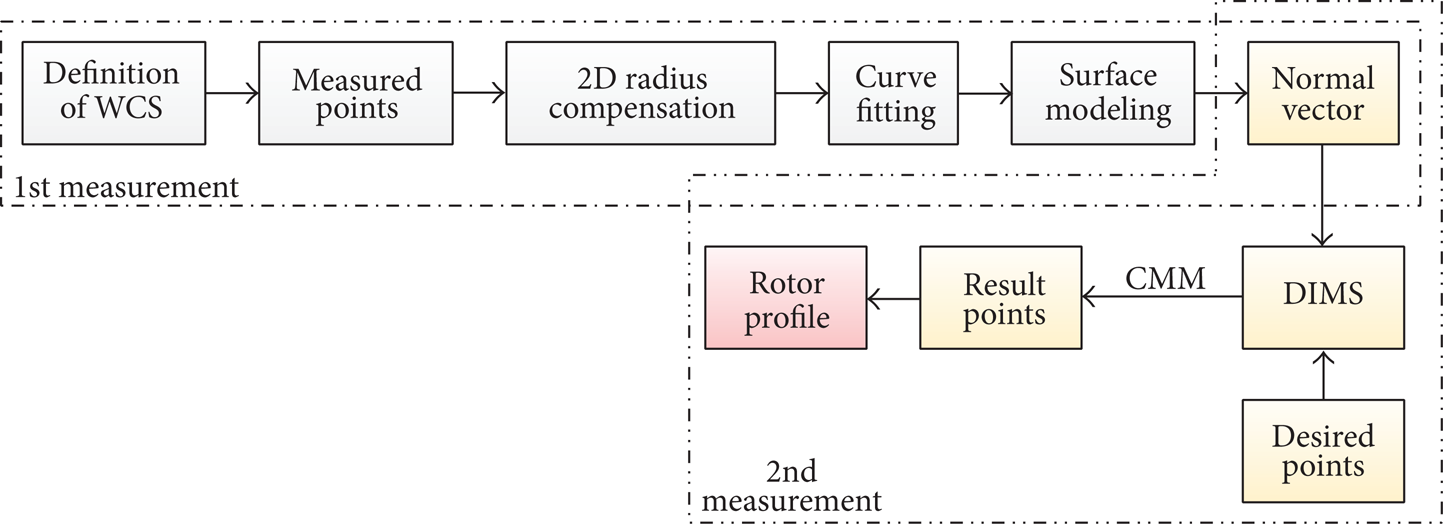
Flow chart for double measurement.

Then the detailed measurement process is elaborated as follows.

3. First Measurement for Screw Rotor

If we have a 3D CAD model of the screw compressor rotor, the normal vectors of any desired points on the CAD model could be calculated theoretically and ensure the accuracy of the probe radius compensation. So it is necessary to measure an unknown screw rotor at first to construct a 3D CAD model as accurate as possible.

Here, in order to construct the 3D CAD model of rotor, its essential attributes such as rotor profile and helical pitch should be calculated firstly, which are presented as follows.

3.1. Definition of WCS

Whether the workpiece coordinate system (WCS) was built exactly and properly would impact following measuring accuracy greatly.

The unknown screw compressor rotor which is measured in this paper is shown in Figure 2. According to the shape and length of screw rotor, it is usually fixed horizontally or vertically. Because the length of screw rotor is proper for measuring stroke of CMM used in this paper, rotor is fixed vertically and the probe is adjusted to the horizontal position. Thus some needed rotor profiles in one groove could be measured in one measuring process and in single clamping.

Figure 2:

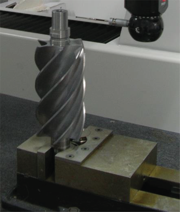
Measured unknown screw rotor and its clamping method.

According to the structural analysis of screw compressor rotor, it is obvious that the rotor itself is a rotational part, so its rotation axis can be identified as the z-axis of WCS. As for the coordinate origin, it is more reasonable to be located on the end face of the rotor. After z-axis and the coordinate origin are defined, corresponding measured elements then should be indicated for the definition of WCS, which mainly could be planes and cylinders, as shown in Figure 3. As a result, the rotation axis of screw rotor is defined as z-axis of WCS. Vertical direction of the plane which is parallel to z-axis, denoted by PL₂ in Figure 3, is defined as y-axis of WCS. The intersection point between z-axis and end face, denoted by PL₁ in Figure 3, is defined as the coordinate origin of WCS, denoted by O in Figure 3.

Figure 3:

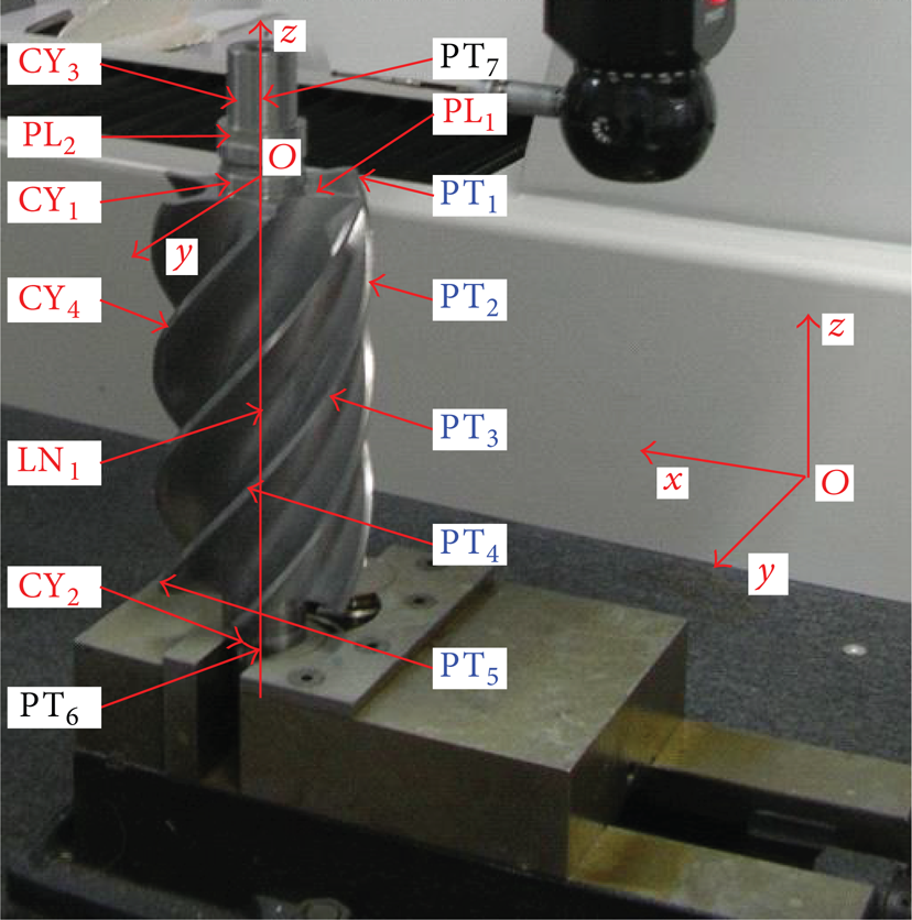
Definition of WCS.

In fact, the most important step for the definition of WCS is the confirmation of z-axis because its accuracy will impact the measuring precision of rotor profile greatly. Usually, several elements are used to define the z-axis of WCS, such as the axes of cylinders denoted by CY₁, CY₂, CY₃, and CY₄ as shown in Figure 3:

CY₁: the short cylinder near the upper part of the working range of the screw rotor;

CY₂: the short cylinder near the lower part of the working range of the screw rotor;

CY₃: the long cylinder at the end of the screw rotor;

CY₄: the outer cylinder of the screw rotor.

In order to analyze the definition accuracy of WCS determined by measured elements mentioned above, the following experiment is designed in time. Firstly, five equidistant points along with helix, denoted by PT₁, PT₂, PT₃, PT₄, and PT₅, are measured in the valid working range of the outer cylinder. Then the vertical distances from these five points to z-axes determined by CY₁, CY₂, CY₃, and CY₄ are figured out, respectively, which are shown in Table 1.

Table 1:

Vertical distances from points to z-axes.

	CY₁	CY₂	CY₃	CY₄

PT₁	24.0135	23.9667	24.0058	24.0242
PT₂	24.0278	23.9743	24.0162	24.0203
PT₃	24.0389	23.9803	24.0255	24.0334
PT₄	24.0526	24.0032	24.0381	24.0235
PT₅	24.0604	24.0055	24.0415	24.0225

Mean	24.0386	23.986	24.0254	24.0248
Limit deviation	0.0469	0.0388	0.0357	0.0131

With multiple measurements, the radius of outer cylinder CY₄ of screw rotor is calibrated to R = 24.0059 mm, which is represented by purple line as shown in Figure 4. The distribution of distances between measured points and z-axes is shown in Figure 4, too.

Figure 4:

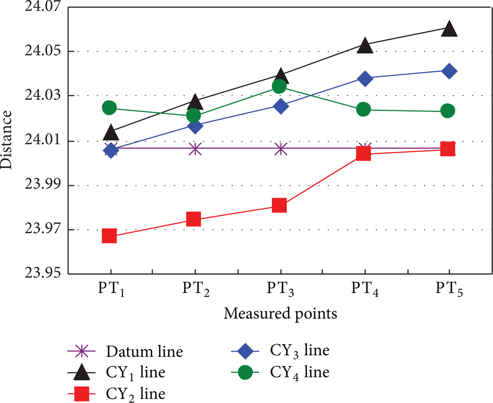
Distribution of distances between measured points and z-axes.

Figure 4 indicates the following.

Because axial length of CY₁ is very short and the machining error of CY₁ is not avoidable, the distance from CY₁ line to datum Line is very large. So the cylinder CY₁ is unsuitable to be used as measured element to define the z-axis of WCS.

The nearer the measured point is to measured element which is used to define the z-axis, the closer the distance from measured point to z-axis is to calibration value R. The farther the measured point is to measured element which is used to define the z-axis, the wider the distance from measured point to z-axis is to calibration value R. If z-axis is defined by CY₂, the distance from PT₅ to z-axis will be closer to R, and if z-axis is defined by CY₃, the distance from PT₁ to z-axis is closer to R.

If z-axis is defined by CY₄, the distances from measured points to z-axis are similar and steady, but unfortunately, all corresponding values are bigger than R.

For these reasons, it is more reasonable to define the z-axis through the central point of CY₂ and CY₃. The specific steps are as follows.

If the central point of CY₂ is denoted by PT₆ and the central point of CY₃ is denoted by PT₇, the line going through both PT₆ and PT₇, denoted by LN₁, could be defined as z-axis.

In this situation, the distances from the five measured points to LN₁ fluctuate near 24.0058 mm, which is very close to the calibration value R. The difference between these two values is only about 1 μm and the defining precision of z-axis is greatly improved.

Each defined coordinate axis and origin of WCS, O, are shown in Figure 3.

3.2. Pretreatment of Point Sets of Measured Rotor Profile

Based on the WCS set up above, each given point set of rotor profile in a single spiral groove is measured at given z. According to the specific function of CMM used in this paper, spline measurement mode (SMM) is adopted, so that the rotor profile is measured automatically and efficiently in one clamping process. In this paper, two point sets of rotor profiles at z = − 20 mm and z = − 130 mm are measured, respectively, as shown in Figure 5.

Figure 5:

Two point sets of rotor profiles at respective z.

3.2.1. Elimination of Outliers

In the measuring process, various outliers emerge due to inevitable noise and fluctuation, which affect the measuring accuracy of CMM and have to be removed before 3D modeling.

Difference in chord height (DCH) algorithm is widely used to solve this problem because of its simpleness and efficiency. However, its removal efficiency depends entirely on the given allowance ε. If ε is too big, part of outliers, which must be removed, cannot be removed. As a result, fairness of reconstructed CAD modeling based on these points will be impacted. If ε is too small, part of normal points (pseudooutliers) which should be maintained will be removed. As a result, authenticity of reconstructed CAD modeling based on these points will be impacted, too. Empirically, ε is usually set as the measuring accuracy of workpiece. Here, ε = 0.02 mm.

The solution for improving DCH includes two aspects. Firstly, a reasonably bigger allowance ε is set to avoid removing pseudooutliers. In this paper, new ε is twice larger than ε. That is, ε_n = 2ε. Then, a new removal criterion, which is called ratio of chord height (RCH), is presented to remove the outliers once more.

Accordingly, a specific algorithm called difference in ratio of chord height (DRCH) is presented in this paper. The specific algorithm is shown as follows.

Step 1. Remove distinct outliers directly.

Step 2. [DCH] Draw chord P_t1P_t3, and calculate vertical distance h₁ from P_t2 to chord P_t1P_t3.

If h₁ ≥ ε_n, then point P_t2 should be identified as an outlier and removed. Then Step 2 is executed again with points P_t1, P_t3, and P_t4.

If h₁ < ε_n, then go to Step 3.

Step 3. [RCH] Draw chord P_t1P_t4, calculate vertical distance h₂₁ from P_t2 to chord P_t1P_t4 and h₂₂ from P_t3 to chord P_t1P_t4, and then calculate the ratios of chord heights:

η_{1} = \frac{h_{21}}{h_{22}}, η_{2} = \frac{h_{22}}{h_{21}} .

(1)

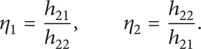
Set the threshold of the ratio of chord height as η.

If η₁⩾η, point P_t2 can be identified as outlier and removed. Then jump to Step 2 and execute it again with points P_t1, P_t3, and P_t4.

If η₂⩾η, point P_t3 can be identified as outlier and removed. Then jump to Step 2 and execute it again with points P_t1, P_t2, and P_t4.

If η₁ < η or η₂ < η, neither P_t2 nor P_t3 is outliers, then jump to Step 2 and execute it again with points P_t3, P_t4, and P_t5.

Step 4. End.

Sketch map for this improved difference in ratio of chord height (DRCH) algorithm is shown in Figure 6. Because the allowance ε_n is set reasonably bigger, removal of pseudooutliers can be prevented effectively where the curvature fluctuates greatly.

Figure 6:

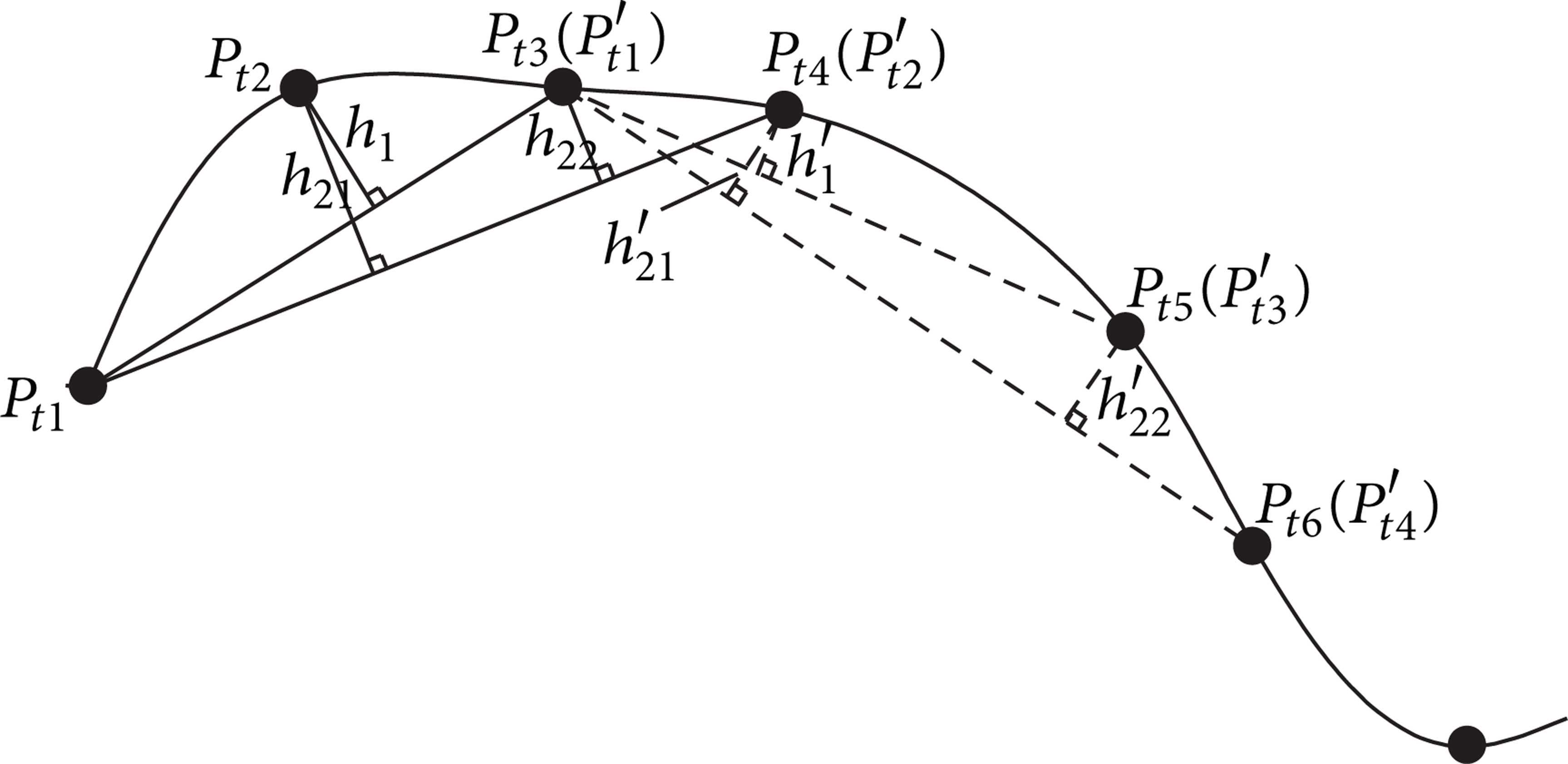
Sketch map for difference in ratio of chord height.

It is important to note that the threshold of the ratio of chord height, η, is also an experience value, usually belongs to [1.5, 2], and should be adjusted flexibly according to the practical situation. However, DRCH algorithm is more robust than usual DCH because of new removal criterion, RCH.

Figure 7 is a point set with some outliers, as shown in Figure 7(a). After DCH with ε = 0.02 mm, six points are removed, as shown in Figure 7(b). Set ε_n = 2ε = 0.04 mm and only one point is removed after DCH, as shown in Figure 7(c). Obviously, outliers are not removed thoroughly in Figure 7(c). By DRCH presented in this paper with ε_n = 0.04 mm and η = 1.6, two real outliers are removed, as shown in Figure 7(d).

Figure 7:

Comparison of DCH and DRCH with different parameters.

So, this adaptable and general algorithm has achieved a fine effect in this paper.

3.2.2. Two-Dimensional Radius Compensation

Based on this measuring coordinate system, two point sets of rotor profile in a whole tooth space at z = − 20 mm and z = − 130 mm are measured in a single measuring process. Because the normal vectors of measured points are unknown, measured points could only be compensated in the approaching direction automatically, which is just a 2D radius compensation and has the inevitable theoretical error. The principle of radius compensation is shown in Figure 8.

Figure 8:

2D probe radius compensation.

Here P₁ is measured points and P₂ is compensated point. The theoretical error δ then is expressed by

δ = R (\frac{1}{\cos α} - 1) .

(2)

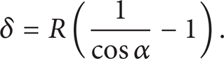
In (2), α is the angle between the axis of the probe and the measured surface normal. R is probe radius.

According to (2), compensation error is impacted by angle α greatly. In fact, because the measured surface of screw rotor is helical, the angle α varies with the different measured points. As a result, it is very difficult to take the compensation error under control. The larger the angle α is, the larger the compensation error is, as shown in Figure 9. Thus, second measurement which will be discussed in Section 4 is necessary to eliminate theoretical compensation error by 3D radius compensation.

Figure 9:

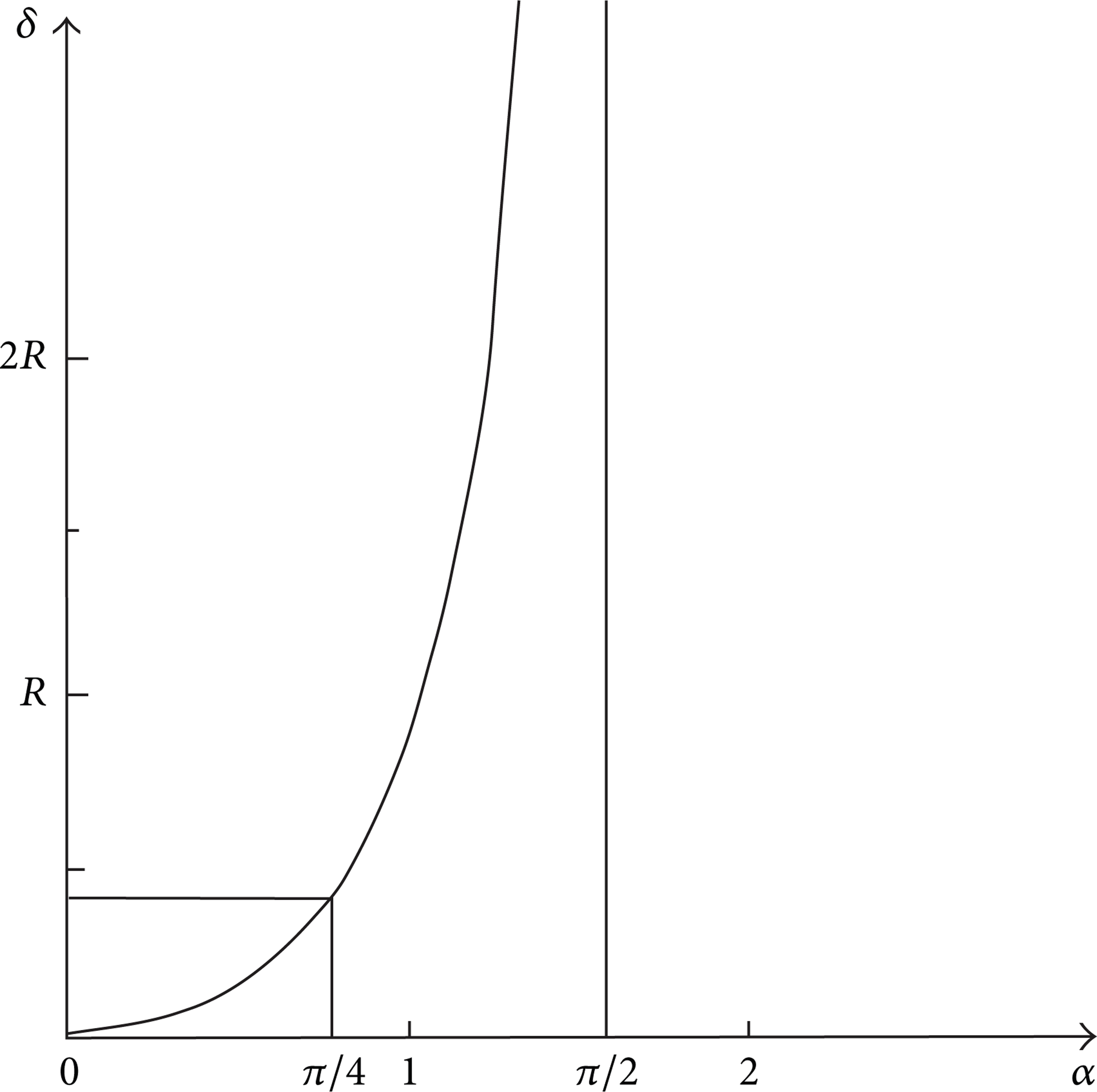
Impact of α on δ.

3.2.3. Interpolation of Sharp Corner of Rotor Profile

The probe radius used in this paper is R = 1 mm. At the place where there is a sharp intersection between two curves or the place where the curves fluctuate wildly, as shown in Figure 10(a), part of curves cannot be measured because of the interference with probe and curves themselves in the measurement process. In this section, probe feeding direction will remain unchanged. When point A is measured, the CMM receives the coordinate data of the center of probe, A′, and the measured point A can be figured out successfully according to the radius compensation algorithm. But when desired point B is measured and the probe is fed at the given same direction, point C will be touched firstly instead of point B because of probe radius, so the CMM will receive the coordinate data of point C′ instead of point B′. After radius compensation, the measuring result of measured point B will be replaced with the point D. According to Figure 10(a), we can find that the measuring error BD is so large that it cannot be accepted.

Figure 10:

Interpolation of sharp corner of rotor profile.

In fact, as shown in Figure 10(b), for a given probe radius, part of curves expressed by OE and OF cannot be measured successfully. The smaller the probe radius is, the shorter the unmeasurable curves are. In addition to reducing the probe radius, curves interpolation could also be adopted to predict the result of unmeasurable curves. As shown in Figure 10(c), interpolated points (little red crosses) can be calculated by interpolated curves OEG and OFH. The intersection point of these two interpolated curves is point O, which is a very important characteristic point for unknown rotor profile.

After several significant steps, such as measurement, probe compensation, and interpolation, are finished, the measured point sets of rotor profile can be obtained, which is shown in Figure 11(a).

Figure 11:

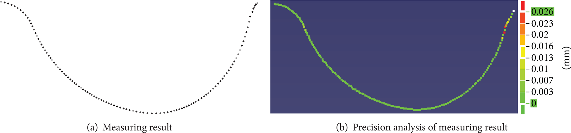
Measured point set of rotor profile and its precision analysis.

Comparing this point set to the original one, as shown in Figure 11(b), the maximum error is 0.026 mm. Obviously, this accuracy cannot meet the engineering requirement mentioned in first section. The reason is the inevitable 2D radius compensation. So a 3D radius compensation will be studied in Section 4 to resolve this problem.

3.3. Indirect Measurement of Screw Pitch

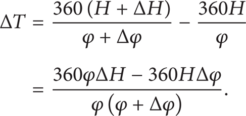
Screw pitch is another intrinsic property of screw compressor rotor. Screw pitch, T, is usually equivalent to the distance it advances in the direction of z axis after rotor profile revolves round z -axis one circle (360°). Thus, screw pitch can be figured out by measuring rotation angle, φ, around z -axis between two rotor profiles at a distance of H, as shown in Figure 12

T = \frac{360}{φ} H .

(3)

Figure 12:

Solution of screw pitch.

For (3), we firstly analyze the influence to the measuring accuracy of screw pitch T caused by the different values of φ and H

\begin{matrix} Δ T = \frac{360 (H + Δ H)}{φ + Δ φ} - \frac{360 H}{φ} \\ = \frac{360 φ Δ H - 360 H Δ φ}{φ (φ + Δ φ)} . \end{matrix}

(4)

Because φ is much larger than Δφ,

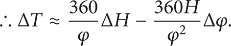
∴ Δ T \approx \frac{360}{φ} Δ H - \frac{360 H}{φ^{2}} Δ φ .

(5)

From (5), we can find that the larger φ is, the smaller ΔT is and the higher the measuring accuracy of screw pitch T is. From (3), H is proportional to φ, so, in order to improve the measuring accuracy of screw pitch T in this measurement process, H should be taken as large as possible.

Concrete calculating method is described as follows. Firstly, measure two rotor profiles, C₁ and C₂, at the distance of H in the direction of z axis in a single process. Secondly, calculate rotation angle, φ, around z-axis between these two rotor profiles. Then, the screw pitch can be figured out easily by (3). In order to ensure the convenience of measurement and the accuracy of calculation, some following measures are taken in this paper.

In order to measure these two profiles in a single process without adjustment of probe direction, C₂ is replaced by C₃. The analysis shows that the angle of C₂ and C₃ around z-axis is 120°. If C₃ rotates 120° clockwise, it is equal to C₂.

In order to calculate rotation angle of C₁ and C₂, φ, around z-axis accurately, C₂ is projected onto the vertical plane of the z-axis, which is determined by C₁, expressed by C₄, as shown in Figure 12. Then, the angle of C₁ and C₂ is replaced by the angle of C₁ and C₄, which is easier to calculate.

Because of the lack of reference points, more angles are calculated at the same time to improve the accuracy of angle φ. Draw five concentric circles with center at O₁. The intersection points of concentric circles and C₁ are denoted by P₁₁, P₁₂, P₁₃, P₁₄, and P₁₅. The intersection points of concentric circles and C₂ are denoted by P₂₁, P₂₂, P₂₃, P₂₄, and P₂₅, as shown in Figure 13. The angle between O₁P₁₁ and O₁P₂₁ is φ₁, the angle between O₁P₁₂ and O₁P₂₂ is φ₂, the angle between O₁P₁₃ and O₁P₂₃ is φ₃, the angle between O₁P₁₄ and O₁P₂₄ is φ₄, and the angle between O₁P₁₅ and O₁P₂₅ is φ₅. The calculating results are shown in Table 2.

Table 2:

The calculating results of φ.

Angle	φ₁	φ₂	φ₃	φ₄	φ₅

Results (°)	117.349	17.352	117.305	117.344	117.365

Figure 13:

Solution of rotation angle.

So the average value of these five angles can be expressed by

φ = \frac{1}{5} \sum_{i = 1}^{5} φ_{i} .

(6)

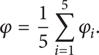
According to the calculating results in Table 2,

\begin{matrix} φ = \frac{(117.349 + 117.352 + 117.305 + 117.344 + 117.364)}{5} \\ = {117.3428}^{°} . \end{matrix}

(7)

At the same time, the distance between the plane of C₁ and C₃, H, can be figured out by the following steps.

Define a least square plane (LSP), z = A, which is determined by C₁ and is perpendicular to z-axis.

The minimum sum of squared distances from point set, C₁, to A is described as

\begin{matrix} Min F = \sum_{i = 1}^{m} {(z_{C_{1} i} - A)}^{2} \\ = \sum_{i = 1}^{m} (z_{C_{1} i}^{2} - 2 A z_{C_{1} i} + A^{2}) \\ = \sum_{i = 1}^{m} z_{C_{1} i}^{2} - 2 A \sum_{i = 1}^{m} z_{C_{1} i} + \sum_{i = 1}^{m} A^{2} . \end{matrix}

(8)

If we take $\partial F / \partial A = - 2 \sum_{i = 1}^{m} z_{C_{1} i} + 2 \sum_{i = 1}^{m} A = 0$ , then $\sum_{i = 1}^{m} z_{C_{1} i} = m A$

∴ A = \frac{1}{m} \sum_{i = 1}^{m} z_{C_{1} i} .

(9)

Similarly, the least square plane (LSP), z = B, which is determined by C₃ is described as

B = \frac{1}{n} \sum_{j = 1}^{n} z_{C_{3} j} .

(10)

Here, m is the number of the point set C₁ and n is the number of the point set C₃.

So, H is figured out,

H = ∥ A - B ∥ = ∥ \frac{1}{m} \sum_{i = 1}^{m} z_{C_{1} i} - \frac{1}{n} \sum_{j = 1}^{n} z_{C_{3} j} ∥ = 110.015 mm .

(11)

Then screw pitch is figured out by (3)

T = \frac{360}{117.3428} \times 110.015 = 337.519 mm .

(12)

On the basis of measured rotor profile and screw pitch, 3D modeling of screw compressor rotor is constructed as accurate as possible, which is shown in Figure 14. To meet the final measuring requirement, more following measures should be taken to improve the measuring accuracy.

Figure 14:

3D modeling of screw compressor rotor.

4. Second Measurement for Screw Rotor

Because radius compensation vectors are unknown in first measurement, 2D compensation with theoretical error is adopted reluctantly. Based on 3D modeling constructed in above section, normal vectors of measured points can be figured out. This is the key to the second measurement.

4.1. Measured Points and Corresponding Normal Vectors

Firstly, calculate intersection curve between plane z = − 20 mm and 3D model of screw rotor (z = − 20 mm is a plane mentioned in Section 3.2). Secondly, scatter this curve into points at the interval of 0.5 mm. These points are the new planned points for second measurement. Then, calculate corresponding normal vectors of these new planned points. Calculated normal vectors of given points are shown in Figure 15 and parts of corresponding values are shown in Table 3.

Table 3:

Part of measured points and corresponding normal vectors.

Number	x	y	z	i	j	k

1	−11.250163	46.662338	−20.001508	−0.310648	0.947468	−0.076173
2	−6.734612	41.607689	−20.002119	0.790704	−0.028680	0.611526
3	−5.963007	34.643340	−20.001998	0.805778	0.230471	0.545532
4	−3.585444	29.426255	−20.00205	0.745639	0.501035	0.439302
5	5.126837	23.392281	−20.002354	0.204608	0.978754	−0.013241
⋮	⋮	⋮	⋮	⋮	⋮	⋮

Figure 15:

Measured points and corresponding normal vectors.

4.2. Three-Dimensional Radius Compensation

According to these new planned points and corresponding normal vectors, a 3D radius compensation can be adopted. Its compensation principle is shown in Figure 16.

Figure 16:

Principle of 3D radius compensation.

In Figure 16, P is the measured point, its normal vector is n, and the measuring points of CMM are P₀. So point P can be compensated by (13).

P = P_{0} - R n .

(13)

Because probe feeding direction is the same as the normal vector of P , it can be ensured that touch point between probe and workpiece is always the measured point. As a result, the measured point is compensated without theoretical error. Final 3D measuring path of second measurement is planned by DIMS language. This path planning program can output compensated points directly. Taking first point in Table 3 as example, some DIMS program for point P (− 11.250163, 46.662338, − 20.001508) with normal vector V (− 0.310648, 0.947468, − 0.076173) is shown as follows:

F(PT1) = FEAT/POINT, CART, −11.250163, 46.662338, −20.001508, −0.310648, 0.947468, −0.076173

MEAS/POINT, F(PT1), 1

PTMEAS/CART, −11.250163, 46.662338, −20.001508, −0.310648, 0.947468, −0.076173

ENDMES

T (1) = TOL/CORTOL, XAXIS, −0.1, 0.1

T (2) = TOL/CORTOL, YAXIS, −0.1, 0.1

T (3) = TOL/CORTOL, ZAXIS, −0.1, 0.1

OUTPUT/FA(PT1), TA (1), TA (2), TA (3)

⋯

4.3. Normalization of Point Sets of Measured Rotor Profile

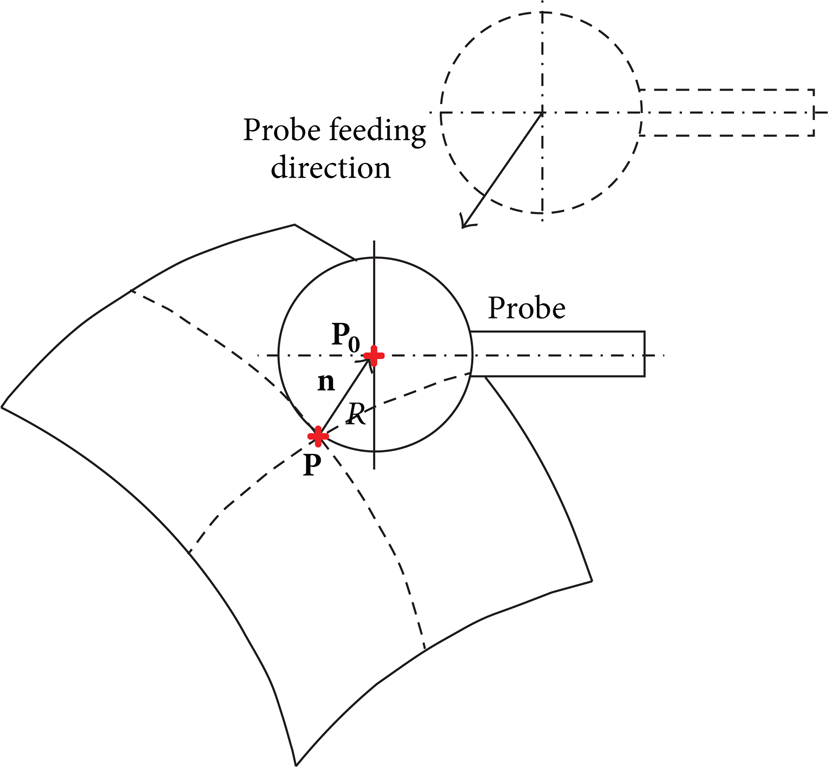
In fact, measured points which are compensated in the direction of normal vectors by above path planning become spatial points and all of them stray from reference plane z = − 20 mm slightly. In order to obtain the accurate sectional profile data, all measured points should also be transformed to plane z = − 20 mm along helix. According to Figure 17, transformation formula of right-hand rotor can be expressed by

\begin{matrix} θ = \frac{(z - z_{0}) \times 360}{T}, \\ x = x_{0} \cos θ - y_{0} \sin θ, \\ y = x_{0} \sin θ + y_{0} \cos θ . \end{matrix}

(14)

Figure 17:

Method for normalization.

Here, P₀ is the result of measured point, P is transformed point on plane z = − 20 mm, θ is the angle between P₀ and P in the direction of z-axis, and T is screw pitch. By this algorithm, the measured points can be transformed onto objective plane at z = − 20 mm. Parts of processed points of rotor profile are shown in Table 4 and these are final measurement result. Precision analysis between final result and original points is shown in Figure 18. Figure 18 shows that after second measurement, maximum measuring error is reduced from 0.026 mm to 0.011 mm. Measuring result is much better than original requirement.

Table 4:

Normalization of point set of measured rotor profile.

Number	Measured points			Transformed points (final result)
Number	x _i	y _i	z _i	x	y	z

1	−6.9110	46.0364	−20.2348	−7.11325	46.00558	−20.0000
2	−6.8207	45.3878	−20.2296	−7.01456	45.35824	−20.0000
3	−6.7288	44.7733	−20.2132	−6.906368	44.74625	−20.0000
4	6.7480	44.1798	−20.2125	−6.922674	44.15276	−20.0000
5	−6.8346	43.5606	−20.2041	−6.999986	43.53433	−20.0000
6	−6.9037	42.9106	−20.1936	−7.058234	42.88545	−20.0000
7	−6.9443	42.2598	−20.1912	−7.094647	42.23482	−20.0000
8	−6.9758	41.6183	−20.1926	−7.124953	41.59303	−20.0000
9	−6.9941	40.9745	−20.1871	−7.136728	40.9499	−20.0000
10	−6.9824	40.3247	−20.1719	−7.111371	40.30215	−20.0000
⋮	⋮	⋮	⋮	⋮	⋮	⋮

Figure 18:

Precision analysis of final result.

Because 3D radius compensation is adopted in the process of second measurement, theoretical compensation error is eliminated. If all of these measuring specifications are observed in the measuring process, measurement accuracy of rotor profile can be ensured and accepted.

5. Conclusion

In this paper, a double measurement method is presented to measure a rotor profile of unknown screw compressor accurately. This method includes two steps. The first step focused on constructing an accurate 3D CAD model. The second step focused on 3D measuring with setting points and their normal vectors based on 3D model.

This research can be summarized as follows.

Workpiece coordinate system is established according to the structural features of screw compressor rotor. So there are no special requirements for positioning accuracy of screw compressor rotor in the process of CMM measuring.

A DRCH method is proposed to eliminate outliers with ε_n = 0.04 mm and η = 1.6.

Sharp corner of rotor profile is measured by curve interpolation.

Screw pitch is measured indirectly with projection and transformation of measured point sets.

Measuring process is automatic with path planning based on DIMS language.

Measurement accuracy is improved greatly from 0.026 mm to 0.011 mm with 3D radius compensation.

This work can be extended to other similar complex parts with free-form surface widely because of its universality and stability.

Conflict of Interests

The authors declare that they do not have any commercial or associative interest that represents a conflict of interests in connection with the work submitted.

Footnotes

Acknowledgments

This work was supported by “the National Natural Science Foundation of China” under Grant no. 51105175, “the Fundamental Research Funds for the Central Universities” under Grant no. JUSRP21006, and “the National Natural Science Foundation of China” under Grant no. 51275210.

References

Sjoholm

Y. C.

, and Kleinboehl

, “Screw compressor rotor profile defined for appropriate CMM measurement,” International Compressor Engineering Conference at Purdue, pp. 16–19, 2012.

Holmes

C. S.

, “Inspection of screw compressor rotors for the prediction of performance, reliability, and noise,” in International Compressor Engineering Conference at Purdue, pp. 12–15, 2004.

Popa

L. C.

Popa

Teodor

, and Baroiu

, “Profiling tool generating method, using the profile measurement of rotor of screw compressor components,” in The Annals of “Dunarea De Jos” University of Galati, Fascicle V, Technologies in Machine Building, pp. 123–128, 2011.

Gnther

Dreier

Pfister

Czarske

Haupt

, and Hufenbach

, “Measurement of radial expansion and tumbling motion of a high-speed rotor using an optical sensor system,” Mechanical Systems and Signal Processing, vol. 25, no. 1, pp. 319–330, 2011.

Matsumato

Kato

, and Kameya

, “Screw compressor and method of manufacturing rotors thereof,” Patent Application Publication, United States, No: 20050147519A1 2005.7.

Keferstein

C. P.

Marxer

Gotti

, “Universal high precision reference spheres for multisensor coordinate measuring machines.,” Manufacturing Technology, vol. 61, pp. 487–490, 2012.

Liang

Zhang

Wang

, and Ge

, “Development of a touch probe based on five-dimensional force/torque transducer for coordinate measuring machine (CMM),” Robotics and Computer-Integrated Manufacturing, vol. 28, no. 2, pp. 238–244, 2012.

Mian

S. H.

and Al-Ahmari

, “Enhance performance of inspection process on Coordinate Measuring Machine,” Measurement, vol. 47, pp. 78–91, 2014.

Barini

E. M.

Tosello

, and De Chiffre

, “Uncertainty analysis of point-by-point sampling complex surfaces using touch probe CMMs. DOE for complex surfaces verification with CMM,” Precision Engineering, vol. 34, no. 1, pp. 16–21, 2010.

10.

D'Amato

Caja

Maresca

, and Gomez

, “Use of coordinate measuring machine to measure angles by geometric characterization of perpendicular planes. Estimating uncertainty,” Measurement, vol. 47, pp. 598–606, 2014.

11.

Krajewski

and Wozniak

, “Simple master artefact for CMM dynamic error identification.,” Precision Engineering, vol. 38, pp. 64–70, 2014.

12.

Sánchez

Ruiz

Padilla

, and Valera

, “Geometrical principles for analysing hypoidal gears in Coordinate Measuring Machines: involutometry, protocols, data interpretation,” Measurement, vol. 45, pp. 2368–2375, 2011.

13.

Ferreira

F. A. M.

Olivab

J. V.

, and Sanchez Perezc

A. M.

, “Evaluation of the performance of coordinate measuring machines in the industry, using calibrated artefacts,” Procedia Engineering, vol. 63, pp. 659–668, 2013.

14.

Bešić

Van Gestel

Kruth

J.-P.

Bleys

, and Hodolič

, “Accuracy improvement of laser line scanning for feature measurements on CMM,” Optics and Lasers in Engineering, vol. 49, no. 11, pp. 1274–1280, 2011.

15.

Wärmeford

Carlson

J. S.

, and Söderberg

, “An investigation of the effect of sample size on geometrical inspection point reduction using cluster analysis,” CIRP Journal of Manufacturing Science and Technology, vol. 3, no. 3, pp. 227–235, 2010.

16.

Lee

R.-T.

and Shiou

F.-J.

, “Calculation of the unit normal vector using the cross-curve moving mask method for probe radius compensation of a freeform surface measurement,” Measurement, vol. 43, no. 4, pp. 469–478, 2010.

17.

Liang

S.-R.

and Lin

A. C.

, “Probe-radius compensation for 3D data points in reverse engineering,” Computers in Industry, vol. 48, no. 3, pp. 241–251, 2002.

18.

Mahmud

Joannic

Roy

Isheil

, and Fontaine

J.-F.

, “3D part inspection path planning of a laser scanner with control on the uncertainty,” CAD Computer Aided Design, vol. 43, no. 4, pp. 345–355, 2011.

19.

Wong

F. S. Y.

Chuah

K. B.

, and Venuvinod

P. K.

, “Automated inspection process planning: algorithmic inspection feature recognition, and inspection case representation for CBR,” Robotics and Computer-Integrated Manufacturing, vol. 22, no. 1, pp. 56–68, 2006.

20.

Zhao