LEDFD: A Low Energy Consumption Distributed Fault Detection Algorithm for Wireless Sensor Networks

Abstract

Detection of faulty nodes and network energy saving have become the hottest research topics. Furthermore, current fault detection algorithms always pursue high detection performance but neglect energy consumption. In order to obtain good fault detection performance and save the network power, this paper proposes a low energy consumption distributed fault detection algorithm (LEDFD), which takes full advantage of temporally correlated and spatially correlated characteristics of the sensor nodes. LEDFD utilizes the temporally correlated information to examine some faulty nodes and then utilizes the spatially correlated information to examine the nodes that have not been detected as faulty through exchanging information among neighbor nodes to determine those nodes' state. Because LEDFD takes the data produced by nodes themselves to detect certain types of faults, which means nodes need not exchange information with their neighbor nodes during the entire detection process, the energy consumption of networks is efficiently reduced. Experimental results show that the algorithm has good performance and low energy consumption compared with current algorithms.

1. Introduction

Wireless sensors networks (WSNs), which consist of large-scale sensor nodes deployed in monitoring regions, are multihop ad hoc networks formed by the wireless communication system. Wireless sensor networks are applied to environmental monitoring and protection, medical care, military target detection and tracking, and so forth [1]. However, sensor nodes are cheap, fragile, and limited by cost and energy and the wireless communication links between sensor nodes are unstable and susceptible to interference. Furthermore, sensor nodes are usually exposed in the environment, vulnerable to physical, chemical, and other external damage. All of these factors readily cause node failure. This makes network monitoring results inaccurate or even entirely wrong. Therefore, in order to obtain accurate monitoring results and take full use of the networks' functionality and complete specific tasks, it is essential and worthy to study fault detection in wireless sensor networks.

Fault detection algorithms for WSNs can be divided into two categories, centralized fault detection and distributed fault detection. The centralized fault detection algorithms usually need the particular node to centralize all collected information and determine the states of other nodes, which easily leads to problems or performance bottleneck, single point of failure, loss of information, and more energy consumptions [2, 3]. Wireless sensor nodes are able to localize themselves with proximity information [4, 5] and communicate and collaborate with each other nearby. Distributed fault detection algorithms require that each node is installed with the fault detection algorithm, uses the data collected by itself or surrounding nodes, and determines its own fault. Distributed fault detection algorithms can be broadly divided into five subcategories further, including the fault detection algorithms based on the majority voting strategy (MV) [6], the fault detection algorithms based on the median value strategy [7], the fault detection algorithms based on the weighted strategy [8, 9], the fault detection algorithms based on the diffusion of decision-making strategy [10–14], and the clustering-based fault detection algorithms [15].

Current fault detection algorithms for WSNs usually have the following problems.

• (1)

They usually seek for high detection accuracy and low false alarm rate but often neglect the energy consumption of the network. Sensor nodes need to communicate with their neighbors several times during fault detection, resulting in high cost energy consumption.

(2)

They only take a few types of fault node into account. So if a new type of fault node increases, their detection performances will decline rapidly.

(3)

They do not take full advantage of the sensor nodes' ability to collect data but just utilize the spatial correlation of the sensor networks to achieve the fault detection, making the complexity of the algorithm higher.

To solve these problems, this paper presents a low energy distributed fault detection algorithm (LEDFD), which uses the temporal correlated characteristics of data collected by sensor nodes to detect some types of fault nodes and removes the nodes from the network. LEDFD reduces the communication times between neighbor nodes and the energy consumption. Then LEDFD utilizes the spatial correlation characteristics of wireless sensor networks to detect the remaining faulty nodes which are not detected in the prior detection. If a node's measured value is the same or close to the measured value of its neighbors whose prior state is normal, the node is considered as a normal node. Otherwise, the node is considered as a fault node. The algorithm also takes into account the nodes which may have transient faults in sensor reading and uses the data collected in a short time to correct the fault data when transient fault readings occur. It can avoid mistaking the normal nodes as fault ones.

2. Related Works

A distributed Bayesian event detection algorithm was proposed in [6]. It adopts the majority voting strategy and requires information exchanged between neighbor nodes to obtain the statistical probability of the event, combining with the failure rate of the node itself to identify events and fault nodes. In [7], a distributed event and event boundary detection algorithm was proposed, which uses the difference between the median measured value of the neighbors and the reading of the node itself to determine whether the node is faulty or not, but as the algorithm in the fault detection phase requires more than one communication with its neighbors, the algorithm's energy consumption is quite large. A weighted average based on a distributed fault detection algorithm was presented in [8]. The algorithm gives each sensor node a weight and makes a determination according to the comparison of the node's reading with the node's neighbors. Reference [9] uses the readings of different sensors to give different weights and combine the median value strategy to determine the final state of the node, which has better performance than the middle strategy algorithms, and low network energy consumption. If a failure occurs, the node's weight will be reduced. But the algorithm does not consider transient faults. In [10] a distributed fault detection algorithm for wireless sensor networks (DFD) was proposed, which uses tests with the node and its neighbors to determine the node's initial state. According to the initial state of the nodes, the final state of the node is determined. The algorithm has higher detection accuracy and lower false alarm rate. But the algorithm requires at least two communications between neighbor nodes, which leads to a high energy consumption cost. Another distributed fault detection algorithm was proposed in [11], which utilizes the results of a node's comparison with its neighbors, the diffusion of decision-making strategy to identify the fault nodes, and time redundancy to deal with transient faults. In [12], according to the difference of multisensors deployed in the same area and related characteristics, a fault detection algorithm based on the DFD algorithm was proposed for multisensor networks. It improves the fault detection accuracy of the gathering area. The algorithm is also suitable for sensor networks with sparse node distribution and high fault rate. A fault detection algorithm based on spatial correlation and time redundancy was proposed in [13]. Transient fault nodes are fault tolerant through time redundancy, and the false alarm rate is reduced. But the algorithm requires spreading the initial state of the nodes to the other nodes, which will cost more energy. Jiang proposed an improved DFD algorithm in [14]. He considers that the DFD algorithm is too harsh to determine the final state of the node under normal conditions. In order to improve the performance of the DFD algorithm, the conditions should be modified. However, DFD and the improved DFD still cause the high energy consumption problem. In [15] a clustering-based fault diagnosis algorithm was proposed, which utilizes the cluster head node to detect the fault nodes in the cluster and uses the optimal threshold to improve the detection accuracy and lessen the impact of fault nodes to the sensor fault probability. However, the algorithm causes the problem of uneven energy consumption.

3. Detection Model

3.1. Network Model

Suppose that the number of sensors randomly deployed in a particular region is N. These sensor nodes have the same communication radius R. Before the implementation of the fault detection algorithm, one node stores at least q pieces of data that it has collected. $s_i$ denotes the number i node in a wireless sensor network. Nodes in $s_i$ 's communication radius are called node $s_i$ 's neighbors. $Neighbor(s_i)$ is used to denote all the neighbors of $s_i$ , $Num(Neighbor(s_i))$ is used to denote the number of neighbors of $s_i$ , and $x_i^t$ is used to denote node $s_i$ 's measured data at time t. Assume that q pieces of data have been collected in the sensors and can be stored in memory before time t, which are $x_i^t,x_i^{t-\mathrm{1}},\dots ,x_i^{t-q-\mathrm{1}}$ , and node $s_i$ and $Neighbor(s_i)$ are in the same or similar environment, which means if node $s_i$ is in the event area, the neighbors of $s_i$ are also in the same event area, and if node $s_i$ is in the normal area, the neighbors of $s_i$ are also in the same normal area.

3.2. Fault Model

If a node is partly faulty, it may still have the abilities of receiving, sending, collecting, and processing data. But the data the node has collected is usually wrong. According to abnormal types of data collected by the node, the failures of sensors can be divided into the following specific types.

• (1)

Fixed faults in readings: sensors with this kind of fault collect data with the same readings and the data are not affected by the environment.

(2)

Random faults in readings: the readings of the nodes are random and uncertain.

(3)

Offset faults in readings: the readings of the nodes deviate from the normal value, and this can change if the environment changes.

(4)

Transient faults in readings: in the process of the data collection, due to hardware features and the effects of environment, transient faults may happen in a short time, resulting in a few data anomalies at one or several times.

In order to improve the utilization of the sensor nodes, we consider the nodes with transient faults as the normal ones, because most of the time, the readings of these nodes are still available.

4. Fault Detection

4.1. Principle of Detection

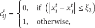
The data that sensors have collected in a short time are temporally correlated, which means the data collected in a short time is the same or similar and it will not change too much. With this feature, we can detect certain types of fault nodes, such as random faults and transient faults. When these faults occur, the value of the data collected in a short time is unstable. However, in order to improve the utilization of the node, we will treat the nodes which have transient faults as normal ones, so when this kind of fault is detected, only by correcting the data collected at the time when faults occur, the normal nodes will not be mistaken as fault ones. Based on the difference between the data collected by nodes, a matrix M is established to determine whether there is a transient fault or a random fault. For the transient fault, the faulty data will be replaced by the normal data collected at other times; thus, it can lower the false alarm rate. However, only using the temporally correlated characteristic is not enough. For example, when fixed faults or offset faults occur, the readings of the nodes meet the temporally correlated feature, but by only using this feature, such types of nodes still cannot be detected, so the neighbors are needed. If most neighbors' data are not similar with the data of the node, then the node is faulty; that is, the sensors have spatial correlation characteristics, which means that, in a small area, most of the sensor nodes have the same or similar readings.

As can be seen from the above analysis, the differences of LEDFD and the current algorithms can be characterized as follows. First, LEDFD uses temporally correlated information to detect some types of node failure and correct some values if necessary, and then detects the remaining fault nodes with the spatial correlation characteristic, while the current algorithms do not use this information or only take advantage of the spatially correlated information to correct some faults and then spread the initial states of the nodes to the other nodes until all the nodes of the network correct their final states.

4.2. Detection Algorithm

After node $s_i$ collects data at time $t,q$ pieces of data can be gained for the latest time. According to (1), the matrix M is established:

$$\begin{array}{l}{M}_{m\times n}\\ =\{\begin{array}{ll}\mathrm{0},\hfill & \text{if}\hspace{0.17em}\hspace{0.17em}\left(\left|x_i^m-x_i^n\right|\le {\xi }_{\mathrm{1}}\right),\hfill \\ \mathrm{1},\hfill & \text{otherwise},\hfill \end{array}\hspace{1em}m,n=\left\{\mathrm{0,1},\dots ,q-\mathrm{1}\right\}.\end{array}$$

(1)

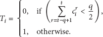
For each row in the matrix M, $c_i^r$ is calculated with

$$\begin{array}{cc}& c_i^r=\{\begin{array}{cc}\mathrm{0},\hfill & \text{if}\hspace{0.17em}\hspace{0.17em}\left(\sum _{j=t-q+\mathrm{1}}^t{M}_{ij}<\frac{q}{\mathrm{2}}\right),\hfill \\ \mathrm{1},\hfill & \text{otherwise},\hfill \end{array}\hspace{1em}\hspace{1em}t-q+\mathrm{1}\le r\le t.\end{array}$$

(2)

The value of $c_i^r$ at time t is corrected with

$$\begin{array}{cc}& c_i^t=\{\begin{array}{cc}\mathrm{0},\hfill & \text{if}\hspace{0.17em}\hspace{0.17em}\left(\sum _{r=t-q+\mathrm{1}}^t{c}_i^r<\frac{q}{\mathrm{2}}\right)\hfill \\ \mathrm{1},\hfill & \text{otherwise}.\hfill \end{array},\end{array}$$

(3)

And any value measured at other time when $c_i^r=0$ can be taken as its value at time t.

Equation (4) is used to determine the initial states of sensor nodes:

$$\begin{array}{cc}& T_i=\{\begin{array}{cc}0,\hfill & \text{if}\mathrm{\hspace{0.17em}\hspace{0.17em}}\left(\sum _{r=t-q+\mathrm{1}}^t{c}_i^r<\frac{q}{\mathrm{2}}\right),\hfill \\ 1,\hfill & \text{otherwise}.\hfill \end{array}\end{array}$$

(4)

If $T_i=0$ , the node $s_i$ may be a normal node and if $T_i=1$ , the node $s_i$ may be a fault one.

For node $s_i$ with state $\mathrm{0}$ , obtains its neighbors' readings whose initial fault states are 0. Then according to (5) and (6), the final state of node $s_i$ is determined:

$$\begin{array}{l}{c}_{ij}^t=\{\begin{array}{ll}\mathrm{0},\hfill & \text{if}\hspace{0.17em}\hspace{0.17em}\left(\left|x_i^t-x_j^t\right|\le {\xi }_{\mathrm{2}}\right)\hfill \\ \mathrm{1},\hfill & \text{otherwise},\hfill \end{array}\end{array}$$

(5)

$$\begin{array}{l}G{T}_i\\ =\{\begin{array}{ll}0,\hfill & \text{if}\hspace{0.17em}\hspace{0.17em}(\sum _{s_j\in Neighbor\left(s_i\right)\hspace{0.17em}\hspace{0.17em}\text{and}\hspace{0.17em}{T}_j=0}{C}_{ij}^t\hspace{1em}\hspace{1em}\hspace{1em}\hfill \\ \hfill & \hspace{1em}\hspace{1em}\hspace{1em}\hspace{1em}<\frac{Num\left(Neighbor\left(s_i\right)\hspace{0.17em}\text{and}\hspace{0.17em}\hspace{0.17em}T=0\right)}{2}\phantom{\sum _{s_j\in Neighbor\left(s_i\right)\hspace{0.17em}\hspace{0.17em}\text{and}\hspace{0.17em}{T}_j=0}{C}_{ij}^t})\hfill \\ 1,\hfill & \text{otherwise}.\hfill \end{array}\end{array}$$

(6)

$Num(Neighbor(s_i)$ and $T=0)$ denote the quantity of nodes whose states are both likely normal and the neighbors of node $s_i$ . $G{T}_i=0$ denotes that node $s_i$ is a normal node. Otherwise, node $s_i$ is a fault one.

For example, supposing $q=5$ and $Num(Neighbor(s_i))=5$ , the q pieces of data that the node $s_i$ collects at time t and before are $\{x_i^t,x_i^{t-1},x_i^{t-2},x_i^{t-3},x_i^{t-4}\}$ , whose values are $\{60.12,30.23,31.54,10.68,30.87\}$ . The node $s_i$ 's neighbors' readings at time t are $\{x_1^t,x_2^t,x_3^t,x_4^t,x_5^t\}$ , whose values are $\{70.22,31.35,65.79,30.84,31.10\}$ , and ${\xi }_{\mathrm{1}}={\xi }_2=2$ . Then according to (1), matrix M is established as

$$\begin{array}{cc}& M_{5\times 5}=\left(\begin{array}{cccc}0& 1& 0& \begin{array}{cc}0& 1\end{array}\\ 1& 0& 1& \begin{array}{cc}1& 1\end{array}\\ 0& 1& 0& \begin{array}{cc}0& 1\end{array}\\ \begin{array}{c}0\\ 1\end{array}& \begin{array}{c}1\\ 1\end{array}& \begin{array}{c}0\\ 1\end{array}& \begin{array}{c}\begin{array}{cc}0& 1\end{array}\\ \begin{array}{cc}1& 0\end{array}\end{array}\end{array}\right).\end{array}$$

(7)

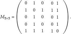
According to (2), $c_i^r=\{0,1,0,0,1\}$ and $t-4\le r\le t\hspace{0.17em}(t\ge 4)$ . According to (3), the value of $c_i^t$ is corrected to 0, and then $c_i^r=\{0,1,0,0,0\}$ . The measured value at time r when $c_i^r=0$ is used to update $x_i^t$ , and $x_i^t=x_i^{t-1}$ . That is, $x_i^t=30.23$ . According to (4), node $s_i$ 's initial fault state can be identified as $T=0$ , which denotes that node $s_i$ may be normal. Then the algorithm gains node $s_i$ 's neighbors' data at time t. Equation (6) shows that $G{T}_i=0$ and node $s_i$ 's final state is normal.

As can be seen from the example, the algorithm is very effective for detection of transient faults and random faults. The algorithm can at most tolerate up to $q/2$ transient faults.

The pseudocode of LEDFD is shown as Pseudocode 1.

Pseudocode 1

For every node $s_i$ in sensor networks ( $i=\mathit{1,2},\dots ,N$ )

Step  1. Create M using the following method

1:   For (every q times before time t including the time t)

2:   IF $\left|x_i^m-x_i^n\right|$ ≤ ${\xi }_{\mathit{1}}$ THEN

3:     $M_{mn}=\mathit{0}$ ;

4:   ELSE $M_{mn}=\mathit{1}$ ;

Step  2. Generate test $c_i^r$

1:   IF ${{\displaystyle \sum }}_{j=t-q+\mathit{1}}^t{M}_{ij}<q/\mathit{2}$  THEN

2:    $c_i^r=\mathit{0}$ ;

3:   ELSE $c_i^r=\mathit{1}$ ;

Step  3. Correct $c_i^t$

1:   IF ${{\displaystyle \sum }}_{r=t-q+\mathit{1}}^t{c}_i^r<q/\mathit{2}$ and $c_i^t=\mathit{1}$ THEN

2:    $c_i^t=\mathit{0}$ ; $x_i^t=x_i^{t-k}$ ;

    //( $(t-k)\in [t-q+\mathit{1},t]$ and $c_i^{t-k}=\mathit{0}$ );

3:   ELSE IF ${{\displaystyle \sum }}_{r=t-q+\mathit{1}}^t{c}_i^r\ge q/\mathit{2}$ and $c_i^t=\mathit{0}$ THEN

4:    $c_i^t=\mathit{1}$ ; $x_i^t=x_i^{t-k}$ ;

    //( $(t-k)\in [t-q+\mathit{1},t]$ and $c_i^{t-k}=\mathit{1}$ );

Step  4. Generate a state value $T_i=\mathit{0}$ based on the value of $c_i^r$

1:   IF ${{\displaystyle \sum }}_{r=t-q+\mathit{1}}^t{c}_i^r<q/\mathit{2}$  THEN

2:    $T_i=\mathit{0}$ ;

3:   ELSE $T_i=\mathit{1}$ ;

Step  5. For the nodes' with state value $T_i=\mathit{0}$ , test every member of their neighbors

to generate test $c_{ij}^t$   {0, 1} using the following method:

1:   IF $\left|x_i^t-x_j^t\right|$ ≤ ${\xi }_{\mathit{2}}$  THEN

2:    $c_{ij}^t=\mathit{0}$ ;

3:   ELSE $c_{ij}^t=\mathit{1}$ ;

Step  6. Make the final decision of the nodes' state ${GT}_i$

1:   IF ${\displaystyle \sum }_{s_j\in Neighbor\hspace{0.17em}\hspace{0.17em}\left(s_i\right)\hspace{0.17em}\hspace{0.17em}\text{and}{\hspace{0.17em}\hspace{0.17em}T}_i=\mathit{0}}{C}_{ij}^t<Num(Neighbor\left(s_i\right)\hspace{0.17em}\hspace{0.17em}\text{and}\hspace{0.17em}\hspace{0.17em}T=\mathit{0})/\mathit{2}$  THEN

2:    ${GT}_i=\mathit{0}$ ;

3:   ELSE ${GT}_i=\mathit{1}$ ;

The algorithm utilizes the historical data that sensors have sensed to determine the nodes' initial state. If the data are stable in a short time (little changed), then the node may be normal. Otherwise, the node may be faulty. That is, only with the sensor nodes' own data, some fault nodes can be identified. After the initial determination of the node's state, for the nodes whose initial state is normal, the algorithm makes a further assertion with its neighbor's readings whose initial states are normal. If the measured value of the node is similar to most of its neighbors', it will be determined as a normal node. In the whole implementation process of the algorithm, the faulty nodes which have been identified by the initial detection are no longer able to communicate with other normal nodes, and the algorithm adopts the data from nodes whose initial states are normal. This approach not only makes the algorithm consume less energy, but also lowers the false detection rate. In addition, the transient faults of the nodes are considered. When it occurs, the algorithm will correct the error of readings, which means the algorithm uses the readings of other times instead of the readings of this time, further enhancing the ability of sensor fault tolerance for transient faults.

5. Simulation Experiments and Performance Analysis

5.1. Performance Indicators

To assess the effect of the fault nodes identification, two indicators are usually employed, detection accuracy and false alarm rate.

Detection accuracy (DA) refers to the ratio of the number of correctly identified fault nodes to the total number of actual fault nodes:

$$\begin{array}{cc}& \text{DA}=\frac{\left|F\cap Q\right|}{\left|Q\right|},\end{array}$$

(8)

where F is the set of fault nodes which the algorithm has detected and Q represents the set of actual fault nodes.

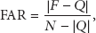
False alarm rate (FAR) refers to the ratio of the number of normal nodes mistaken as fault nodes to the total number of normal nodes:

$$\begin{array}{cc}& \text{FAR}=\frac{\left|F-Q\right|}{N-\left|Q\right|},\end{array}$$

(9)

where N is the total number of nodes in the wireless sensor network.

Most of the energy of the node is consumed by the communication between nodes [16]. So the total number of communications between nodes can be used to represent the total network. Suppose that the average energy consumption is $e_i$ when the node $s_i$ communicates with its neighbors once and the node communication radius is R:

$$\begin{array}{cc}& \text{EC}=\sum _{i=1}^N{e}_i,\end{array}$$

(10)

where $\text{EC}$ is the total network energy consumption.

5.2. Parameter Settings

We built a simulation experimental system of WSNs with JAVA and implemented the following experiments. Matlab was used to complete the performance analysis. During the experiments, 1024 sensor nodes are randomly deployed in a 32*32 square area. Without loss of generality, we assume that the location of each node is known, and all nodes have the same communication radius R, the readings of the nodes in the normal region are subject to the distribution of   $N(\mu ,\sigma )(\mu =35,\hspace{0.17em}\hspace{0.17em}\sigma =1)$ , and the node fault threshold is ${\xi }_{\mathrm{1}}=5$ and ${\xi }_{\mathrm{2}}=3$ . At least 5 pieces $(q=5)$ of data are stored in each sensor node. The value of q is not too high, because the sensor nodes have a limited storage ability. If the value of q is too high, the data may occupy too much storage space. As the fixed faults are similar to the offset faults, we treat both types of faults as the offset fault. The readings of the fault nodes are set as follows: the offset fault readings range from 61 to 70, the random fault readings range from 1 to 100, and the transient fault readings range from 1 to 100. Suppose that the energy consumption of node $s_i$ communicating with its neighbors is $e_i=10^{-5}\hspace{0.17em}\text{J}$ when R is 2. The experimental results are derived from the average value of 100 experiments.

5.3. Experimental Results and Performance Analysis

Figures 1(a), 1(b), and 1(c) show the performance of the algorithms on different average node densities if only offset faults occur. Figures 1(a), 1(b), and 1(c) indicate the performance of each algorithm at density = 7, 10, and 20. From these figures we can see that with the decrease of node density the performance of each algorithm improves. Taking Figure 1(c), for example, when the sensor fault probability is lower than 35%, DFD has higher detection accuracy, and LEDFD proposed in this paper has similar detection accuracy to MV; when the sensor fault probability is higher than 35%, the detection accuracy of DFD quickly decreases compared with LEDFD and MV. However, the DFD algorithm has a lower false alarm rate, while the false alarm rate of LEDFD is between DFD and MV. Taking everything into consideration, only when offset faults occur, LEDFD algorithm performance is between DFD and MV.

Figure 1

The performance of algorithms on different average node densities when only offset faults occur.

Figures 2(a), 2(b), and 2(c) show the performance of the algorithms on different average node densities if only random faults occur. Figures 2(a), 2(b), and 2(c) indicate the performance of each algorithm at density = 7, 10, and 20. From Figure 2, we can see that the average node density has little effect on the detection accuracy, while the false alarm rate decreases with the increase of average node density. For the random faults that sensors may be subject to, LEDFD has good performance even in the case of high sensor probability, and still maintains high detection accuracy and low false alarm rate. This is mainly because the algorithm first checks whether nodes' readings are stable over a short time. If nodes' readings are unstable, there may be a failure, and the data of the random fault sensors are random and unstable. Since the value of the random fault is within 1–100 range, DFD and MV are effective for detection accuracy of such fault, but less effective than LEDFD. Both of them reach more than 94%, and there may be an increase in detection accuracy with the increase of sensor fault probability (such as MV). However, the false alarm rates of DFD and MV will increase with the increase of sensor fault probability. Meanwhile, the false alarm rate of LEDFD is almost zero.

Figure 2

The performance of algorithms on different average node densities when only random faults occur.

Figures 3(a), 3(b), and 3(c) show the relationship between the sensor fault probability and false alarm rate on different average node densities, density = 7, 10, and 20, if only transient faults occur when $q=5$ . As Figure 3 shows, the false alarm rate of all algorithms decreases with the increase of average node density. LEDFD has a very good performance to handle the transient faults, and its false alarm rate is very low. When the sensor fault probability is 50%, the false alarm rate is still less than 5%. This is due to the algorithm which is based on the q pieces of data to determine whether the data collected is right. If it is incorrect, LEDFD will correct it by taking the data at another time to replace the data of the current time. That is why the algorithm has a good fault-tolerant performance for transient faults. Neither DFD nor MV takes the transient faults into account, and consequently they have a high false alarm rate with the increase of sensor fault probability.

Figure 3

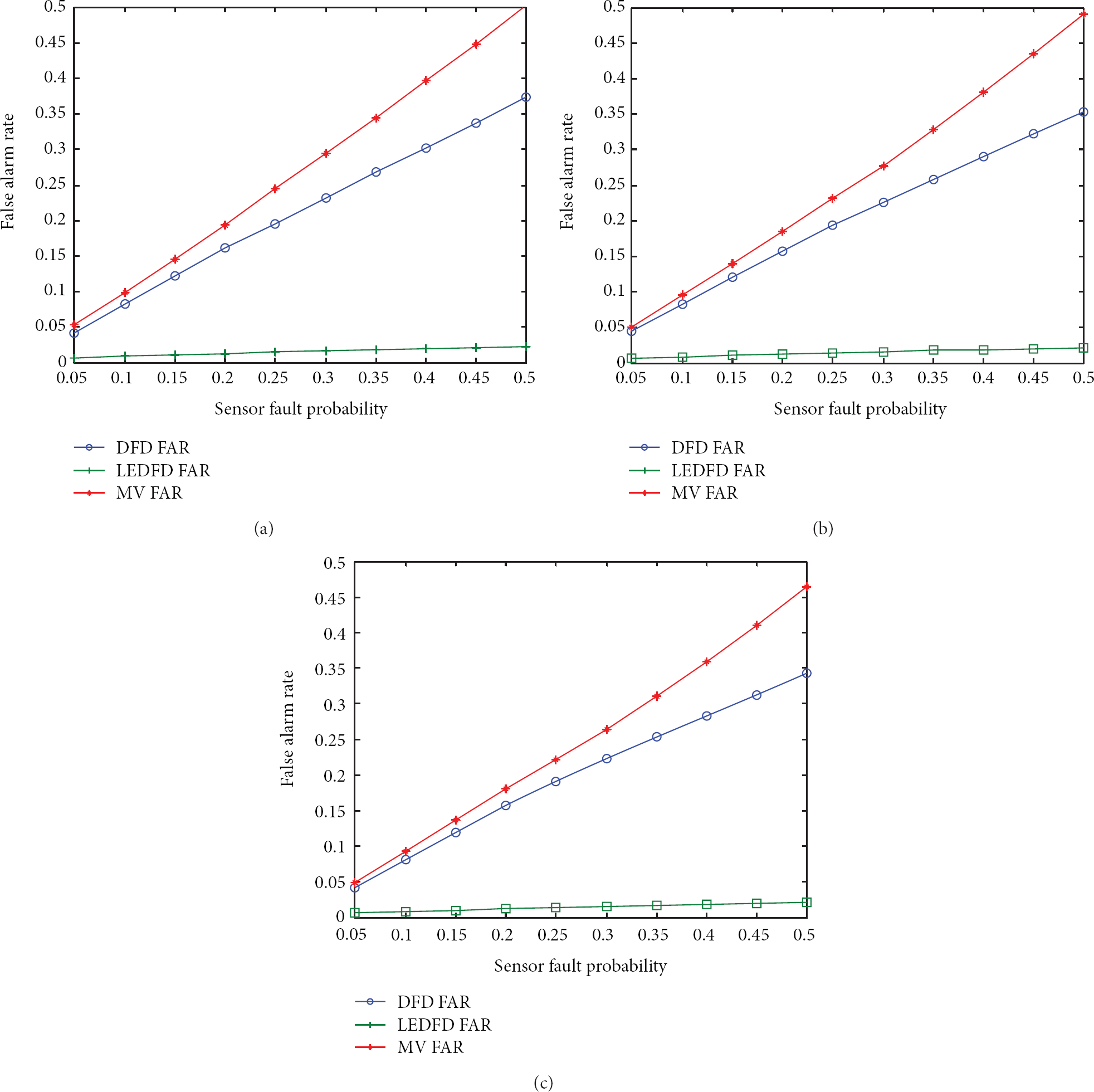
The relationship between the sensor fault probability and false alarm rate on different average node densities if only transient faults occur.

Figures 4(a), 4(b), and 4(c) show the relationship between the sensor fault probability and false alarm rate on different average node densities, density = 7, 10, and 20, when the offset faults, the random faults, and the transient faults occur together randomly. As Figure 4 shows, the detection accuracy of DFD and LEDFD is almost the same. Both of them are higher than MV when the sensor fault probability is below 32%. However, the detection accuracy of DFD decreases rapidly when the sensor fault probability is greater than 32%. The false alarm rate of LEDFD is the lowest among the three algorithms. In short, in mixed fault scenarios, the performance of LEDFD algorithm is up to our expectations.

Figure 4

The relationship between the sensor fault probability and false alarm rate on different average node densities in mixed fault scenarios.

Figure 5 indicates the relationship between energy cost and sensor fault probability of DFD, MV, and LEDFD when the rate of transient faults to the rate of offset faults is 1 : 1, nontransient fault occurs, and the communication radius R is 2. As Figure 4 shows, in the same conditions, DFD has a higher energy cost with the increase of sensor fault probability, for each node needs to communicate with its neighbors at least twice (the first communication is to exchange the initial data collection and the second is to exchange the initial state of each node). However, the final states of the nodes which have not been determined need a third communication. Consistently, the energy cost of DFD is relatively high. For MV, each node only needs to communicate with its neighbors once, so its network energy consumption is moderate. LEDFD first uses the temporally correlated information to make the initial fault detection. In this process, each node does not need to communicate with its neighbors. Only the nodes detected with normal states need to communicate with their neighbors and consume extra energy. Therefore, in case of high sensor probability, fewer nodes are not found faulty through the fault detection and the network's energy consumption is reduced too. In short, the LEDFD algorithm has the advantage of low energy consumption.

Figure 5

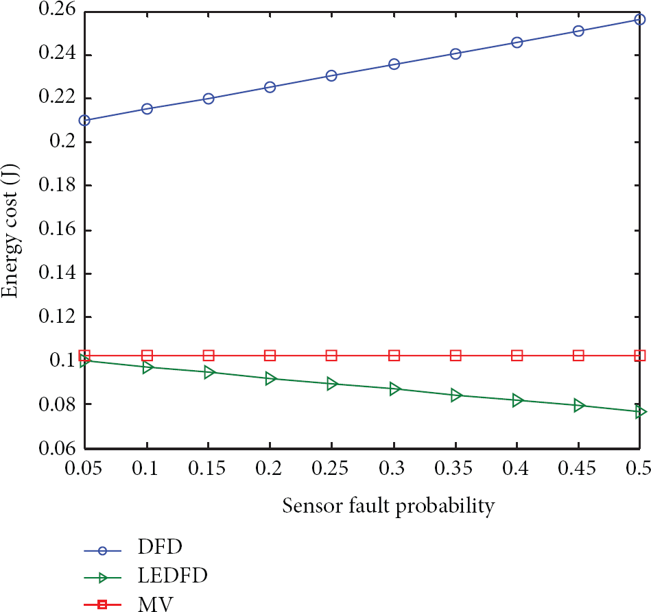
The relationship between energy cost and sensor fault probability of DFD, MV, and LEDFD.

From the above experiments and performance analysis, we obtain the following results.

• (1)

LEDFD shows superior performance, especially for random faults and transient faults, for the LEDFD algorithm fully considers the possible types of node fault, takes advantage of the temporally correlated characteristics of the data collected by the sensor in a short time, determines the stability of the data by establishing symmetric matrices, and detects some fault nodes. The readings of a node with random faults are unstable, so the algorithm is very effective for such faults.

(2)

For transient faults, LEDFD corrects the fault values and makes the false alarm rate very low.

(3)

On the aspect of the LEDFD energy consumption, some of the fault nodes have been detected during the initial phase of detection. During the detection of the remaining nodes, other nodes do not need to communicate with the fault nodes that have been detected, which also reduces communication traffic and saves the network energy consumption.

6. Conclusions

This paper presents a low energy consumption distributed fault detection algorithm for wireless sensor networks. The algorithm takes full advantage of the data characteristics collected by the sensor nodes. LEDFD uses the data sequence collected by the sensor node itself to detect specific types of fault and then uses the neighbors' data further to determine the states of nodes. To various types of faults, LEDFD has the better detection accuracy, lower false positive rate, and less energy consumption. In our future research, we will also consider how to make the fault nodes in the event boundary and other specific circumstances tolerant and implement these algorithms in real applications of wireless sensor network.