Sage Journals: Discover world-class research

Abstract

A CFD model was presented to simulate the distribution of air velocity and temperature in a greenhouse adopting the fan-pad cooling system in summer. The Boussinesq hypothesis was applied for the simulation of gravitation; the k-ε turbulent model and discrete ordinates model were selected to predict the distribution of air velocity and temperature inside greenhouse using the commercial software Fluent. The differences between simulated and measured air temperature varied from 0.9 to 4°C and the differences of air velocity were less than 0.15 m/s, which proved that the CFD method can estimate the distribution of air velocity and temperature in the greenhouse rationally and effectively. The validated CFD model was then used to evaluate the cooling effect and design the installment of fan and pad in terms of the crop size. The results implied that Case 3 and Case 5 should be chosen when the height of crop canopy varies from 2 m to 3 m. When it varies from 1 m to 2 m, all the cases can be effective except Case 1. When the canopy height is below 1 m, all the cases can be selected. This paper suggested that the CFD model can be used as an optimal tool for fan-pad evaporative cooling system in the greenhouse.

1. Introduction

Greenhouse is widely used to create a suitable environment for crop growth. High temperature do harm to the crop, especially in summer. The cooling technique is essential for greenhouse in tropical or subtropical regions, such as natural ventilation, whitening, shade screens, and evaporative cooling [1]. Evaporative cooling is the most efficient way for maintaining lower temperature and increasing humidity in greenhouses [2].

Many researches have been carried out on greenhouse cooling for decades [3]. Chandra et al. conducted an experimental study in a plastic covered greenhouse with fan-pad system for cooling [4]. The climatic variables in a fan-ventilated multispan greenhouse were investigated through experiments [5]. Sánchez-Hermosilla et al. investigated the cooling effect of greenhouse fog system in comparison with conventional spray guns. The experimental results showed that the deposition values on the crop were much lower than the values reached with spray guns [6]. To study the surplus air thermal energy (SATE) in greenhouse, Yang and Rhee operated a greenhouse system to capture and use SATE for cooling and heating inside greenhouse and evaluated its performance. The results showed good energy conservations [7]. Many researchers used mathematical model to evaluate the thermal performance of greenhouse cooling in greenhouse [8]. Mongkon et al. evaluated geothermal cooling ability and studied corresponding parameters in Thailand by mathematical model [9]. Commercial software MATLAB was usually employed for the simulations. Jain and Tiwari developed a mathematical model to study the thermal behavior after evaporative cooling (fan and pad type) in the greenhouse using MATLAB. The cooling system parameters were optimized against the maximum temperature and thermal load leveling in different zones [10]. To predict the temperature gradients along a greenhouse, Kittas et al. proposed a climate model which incorporated the effect of ventilation rate, roof shading, and crop transpiration. The simulation indicated that high ventilation rates and shading contribute to reducing the temperature gradients [11]. In order to maintain a suitable internal temperature, Attar et al. developed a thermal model to investigate the possibility to use the ground thermal energy for the greenhouse heating or cooling. Experiments in a greenhouse integrated with the ground heat storing system were conducted to evaluate the effectiveness of the control system [12]. However, it is still extremely hard to have a clear and comprehensive understanding of its complex character by these traditional methods.

The computational fluid dynamics (CFD) technique provides a better and fast reliable understanding of the flow fields with less labor and cost [1, 13 –15]. Short and Lee used the commercial CFD models to evaluate natural ventilation system alternatives in a multispan greenhouse [16]. The effects of various factors in greenhouses with different ventilation systems were investigated using CFD models [17, 18]. Wang et al. presented a CFD model of a typical plastic greenhouse to explore the inside microclimate distributions [19]. The CFD technique was applied for the study on greenhouse cooling. Kim et al. developed a two-dimensional CFD model to simulate the temperature and relative humidity distributions of a greenhouse with fog-cooling system. The verified model was used to evaluate the cooling efficiency and to find an optimal setup of the fog-cooling system in a multispan greenhouse [20]. Different geometries of evaporative pads can be analysed using CFD technique, and the relationship between air velocity, porosity, and pressure drops was investigated [21]. However, most researchers developed the CFD model for natural ventilated or the fog-cooling system in the greenhouses. There has been relatively little focus on greenhouses equipped fan-pad cooling system in summer using CFD technique.

This paper presents a 3D model of a fan-pad ventilated greenhouse in eastern China. The air temperature and velocity distribution in the greenhouse in summer is simulated using CFD technique. The numerical results are compared with the experiment measured values to verify the validity and efficiency of the CFD model and are also used to optimize the fan-pad evaporative cooling system.

2. Materials and Methods

2.1. Greenhouse Configuration and Measurements

An experimental greenhouse was used to validate and analyze the results obtained from the CFD model. Figure 1 shows the configuration of the greenhouse, which was located in Hangzhou, China (east longitude 120°09′, north latitude 30°14′). The greenhouse was 24 m long, 4 m high at the gutter, and 4.7 m high at the ridge and consisted of 3 spans each 3.2 m wide. The greenhouse was equipped with the external and internal shading screens. The fan-pad evaporative cooling system was applied in the greenhouse, which placed an evaporative pad (9000 mm·100 mm·1500 mm) on the air inlet at the east end and used the two exhaust fans (380 V, 0.75 KW) at the other end of the greenhouse.

Figure 1:

The greenhouse configuration.

In this experiment, the temperature inside the greenhouse was measured and collected at different locations every minute through ten temperature sensors (DS18B12, T1∼T10) and three temperature sensors (HMW61, TH1∼TH3).

The sensors layout is shown in Figure 2. The experiment was conducted from 12:30 to 13:30 on July 23, 2012. During the experimental period, the exhaust fans, evaporative pad, and external shading screen were used, while the side and top windows were all closed.

Figure 2:

The layout of temperature and humidity sensors.

2.2. CFD Numerical Model

The widely used commercial CFD software Fluent 6.3.26 [22] was employed to generate a numerical meshed model for the temperature distribution and air velocity inside greenhouse. The Reynolds-averaged Navier-Stokes equations were solved by finite volume method (FVM) to convert the governing partial differential equations into the equivalent system of discrete algebraic equations [23]. Viscous dissipation term in the energy equation was neglected for the greenhouse with macroscale geometries. The standard k-ε turbulence model had been used to represent ventilation flows. In this model, the turbulent viscosity was computed as a function of the turbulent kinetic energy (k) and the dissipation rate of turbulent kinetic energy (ε). The governing equations are as follows.

Continuity is as follows;

\frac{\partial u}{\partial x} + \frac{\partial v}{\partial y} + \frac{\partial w}{\partial z} = 0.

(1)

Momentum is as follows:

\begin{array}{l} \frac{\partial (ρ u u)}{\partial x} + \frac{\partial (ρ u v)}{\partial y} + \frac{\partial (ρ u w)}{\partial z} = & μ_{e f f} (\frac{\partial^{2} u}{\partial x^{2}} + \frac{\partial^{2} u}{\partial y^{2}} + \frac{\partial^{2} u}{\partial z^{2}}) \\ - \frac{\partial p}{\partial x}, \\ \frac{\partial (ρ v u)}{\partial x} + \frac{\partial (ρ v v)}{\partial y} + \frac{\partial (ρ v w)}{\partial z} = & μ_{e f f} (\frac{\partial^{2} v}{\partial x^{2}} + \frac{\partial^{2} v}{\partial y^{2}} + \frac{\partial^{2} v}{\partial z^{2}}) \\ - \frac{\partial p}{\partial y}, \\ \frac{\partial (ρ w u)}{\partial x} + \frac{\partial (ρ w v)}{\partial y} + \frac{\partial (ρ w w)}{\partial z} = & μ_{e f f} (\frac{\partial^{2} w}{\partial x^{2}} + \frac{\partial^{2} w}{\partial y^{2}} + \frac{\partial^{2} w}{\partial z^{2}}) \\ - \frac{\partial p}{\partial z} - p g β (T - T_{r e f}) \end{array}

(2)

Energy is as follows:

\begin{array}{l} \frac{\partial (p u T)}{\partial x} + \frac{\partial (p v T)}{\partial y} + \frac{\partial (p w T)}{\partial z} \\ = \frac{q}{C_{p}} + \frac{λ_{e f f}}{C_{p}} (\frac{\partial^{2} T}{\partial x^{2}} + \frac{\partial^{2} T}{\partial y^{2}} + \frac{\partial^{2} T}{\partial z^{2}}) . \end{array}

(3)

Turbulent kinetic energy is as follows:

\begin{matrix} \frac{\partial (p u k)}{\partial x} + \frac{\partial (p v k)}{\partial y} + \frac{\partial (p w k)}{\partial z} = Γ_{k} + (\frac{\partial^{2} k}{\partial x^{2}} + \frac{\partial^{2} k}{\partial y^{2}} + \frac{\partial^{2} k}{\partial z^{2}}) \\ + S_{k} . \end{matrix}

(4)

Dissipation rate of turbulent kinetic energy is as follows:

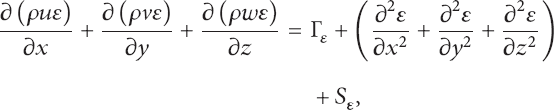
\begin{matrix} \frac{\partial (p u ɛ)}{\partial x} + \frac{\partial (p v ɛ)}{\partial y} + \frac{\partial (p w ɛ)}{\partial z} = Γ_{ɛ} + (\frac{\partial^{2} ɛ}{\partial x^{2}} + \frac{\partial^{2} ɛ}{\partial y^{2}} + \frac{\partial^{2} ɛ}{\partial z^{2}}) \\ + S_{ɛ} . \end{matrix}

(5)

where u, v, w are themean velocity components in x, y, and z directions, respectively. μ_eff is the effective viscosity. T is the air temperature. T_ref is the reference temperature of the air. ρ is the air density. G is the acceleration of gravity. β is the coefficient of thermal expansion: β = 1/T. q is heat source. c_p is the specific heat. λ_eff is the effective thermal conductivity. k is the turbulent kinetic energy. ε is the dissipation rate of turbulent kinetic energy. Λ_k and S_k is the source term for turbulent kinetic energy. Λ_ε and S_ε is the source term for the dissipation rate of turbulent kinetic energy.

The discrete ordinates (DO) model was chosen as a radiation model for the sun light radiation in the greenhouse. The Boussinesq hypothesis was applied to the model for the simulation of gravitation [20].

2.3. Grid Generation

Due to the complicated structure of the greenhouse, the unstructured grid type Tgrid was selected to mesh the greenhouse computational domain in the commercial software Gambit. Local refinement technique was applied to depict the complicated air flow character in the vicinity of the evaporative pad, fans, and walls. Hence, densest meshes presented near these regions to capture the sharp temperature and air velocity gradients in these regions [24, 25]. In order to ensure the independency of the results from grid mesh, several grids with different densities were applied to the computations [26, 27]. Finally, a grid including 189045 cells and 37461 nodes was chosen because it could provide a good compromise between computational speed and the precision of the numerical results (Figure 3).

Figure 3:

Grid generated in the greenhouse computational domain.

2.4. Parameters and Boundary Setting

The walls materials, the air properties inside greenhouse, and other initial conditions were determined based on experimental measurements. Table 1 shows the basic parameters and boundary conditions in the CFD model. The adaptive time stepping method was selected for the iteration of the CFD model.

Table 1:

Basic parameters and boundary conditions in the model.

Properties	Value/unit

Air density	1.225 kg/m³
Thermal conductivity coefficient	0.0225 W/m·k
Thermal expansion coefficient	3.356 × 10⁻³ 1/K
Specific heat	1.005 kJ/kg·k
Viscosity	1.83 × 10⁻⁵ kg/m·s

Glass density	2500 kg/m³
Thermal conductivity coefficient	0.74 W/m·k
Heat transfer coefficient	6.4 W/m²·k

Inlet velocity	0.8 m/s
Outlet velocity	6.0 m/s
Outside radiation	660 w/m²
Ambient temperature	33°C
Ground temperature	28°C

3. Results and Discussion

The fan-pad cooling system was used to maintain a suitable temperature in the greenhouse, especially at the region of crop canopy (the height of 1.2 m from the ground in the experiment). In this study, the air flow contour of two typical sections was selected to analyze the air flow behavior in the greenhouse. Section A was the horizontal section of the greenhouse at the height of 1.2 m (z = 1.2 m). Section B was the longitudinal Section 3 m away from the evaporative pad (x = 3 m).

3.1. Analysis of the Simulation Results

Figure 4 shows the temperature distribution of section A; obvious temperature gradients can be observed at the level of crop canopy. The regions near the walls of the greenhouse have relatively high temperature. The temperature in this section varies from 25.3°C to 26.3°C, which can meet the requirement of crop growth.

Figure 4:

The temperature distribution of section A.

Figure 5 shows the temperature distribution of section B. There is a curtain temperature gradient in the vertical direction. The temperature increases along the height. A strong temperature gradient can be observed near the top, while the temperature changes slightly in the middle as well as near the ground.

Figure 5:

The temperature distribution of section B.

3.2. Validation of the CFD Model

Figure 6 shows the simulated temperatures and air velocity compared with the measured values. The maximum temperature difference between measured and simulated values is 3°C (T6) with a relative error of 8.9%, while the differences from other sensors are less than 2°C. The maximum air velocity difference is 0.15 m/s (TH1) with a relative error of 12%, while the differences from other sensors are less than 0.08 m/s.

Figure 6:

Comparison of temperature and air velocity between the measured and simulated values.

Although there is certain deviation between the simulated and experimental values, the temperature distribution and its variation trend from the simulations are basically in agreement with the experimental results. The numerical simulation is rational, and the CFD model and its corresponding boundary settings are appropriate. And the CFD model can be a good tool for the design and optimization of the fan-pad evaporative cooling system in the greenhouse.

3.3. Optimal Location of the Fan and Pad

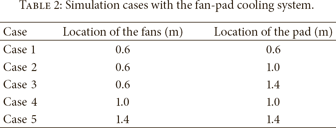
Prior parametric studies revealed that height of the evaporative pad and fans were found sensitive to the cooling effect inside greenhouse [10]. The evaporative pad and fans are usually installed at low position in greenhouses, which may result in a large temperature gradient (more than 20°C) in the vertical direction in summer. The fans and pad are usually installed at the height of 0.6 m in the greenhouse. When the height of the crop canopy is lower than 2 m, the fan-pad cooling system can maintain a suitable temperature for crop growth (lower than 30°C). However, for crops with higher canopy height such as cucumber and tomato, the evaporative cooling system with conventional installment may not be appropriate since the temperature of crop canopy exceeds the suitable range. Therefore, the fans and pad should be located at the higher position for some crops. To meet the environment requirement for crop growth with different sizes, the cooling effect of the fan-pad system in different locations was analyzed. The cooling effect at crop canopy was discussed in different ranges based on the height of various crops, including the range below 1 m, 1 m∼2 m, and 2 m∼3 m. Table 2 shows five cases for different location of the fans and evaporative pad.

Table 2:

Simulation cases with the fan-pad cooling system.

Case	Location of the fans (m)	Location of the pad (m)

Case 1	0.6	0.6
Case 2	0.6	1.0
Case 3	0.6	1.4
Case 4	1.0	1.0
Case 5	1.4	1.4

All the cases above were constructed and simulated using CFD in the same condition, the results are shown in Figure 7.

Figure 7:

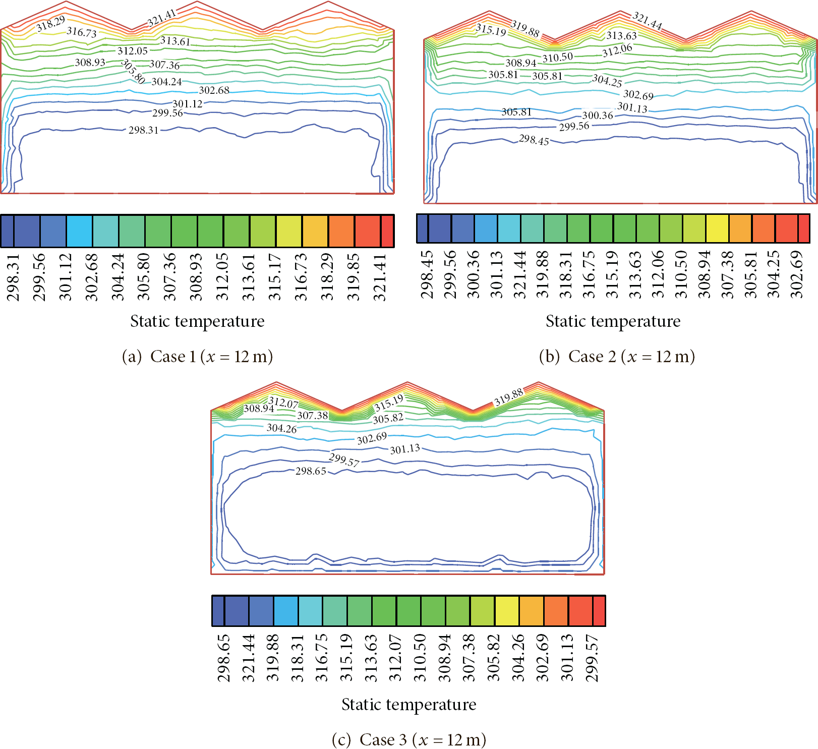
The temperature distribution in Case 1, Case 2, and Case 3.

Figure 7 shows the temperature distribution of a longitudinal section in the greenhouse (x = 12 m). In Case 1, Case 2, and Case 3, the fans locate at the same level while the evaporative pad locates at different height. There are obvious temperature gradients in the vertical direction, and the temperature varies firmly near the top in the greenhouse. In Case 1, the temperature of the region above 2 m is higher than 30°C, which is not suitable for crop growth. In Case 2, the cooling effect is better than Case 1, but the temperature still exceeds 30°C at the region above 2.5 m. Case 5 creates a suitable temperature (25.6°C∼30°C) for the region below 3 m.

The fans and pad are installed at the same level in Case 1, Case 4, and Case 5, respectively. Figure 8 shows the temperature distribution of these cases. In Case 4, unsuitable temperature (higher than 30°C) can be observed at the region above 2.5 m. It suggests that Case 5 can also be a good choice for crops with canopy lower than 3 m since the temperature varies from 25.2°C to 29.0°C in Case 5.

Figure 8:

The temperature distribution in Case 1, Case 4, and Case 5.

The results imply that Case 3 and Case 5 should be chosen when the height of crop canopy varies from 2 m to 3 m. When it varies from 1 m to 2 m, Case 2, Case 3, Case 4, and Case 5 can be effective for greenhouse cooling. When the height of crop canopy is below 1 m, all of the cases can meet the environment requirement for crop growth.

4. Conclusions

This paper presented a CFD model to analyze the air flow characters inside greenhouse using Fluent. A greenhouse in Hangzhou was selected as the experiment greenhouse. The data obtained from the temperature sensors installed in the greenhouse was used to verify the CFD model. The simulation was in good agreement with the experimental results. The differences of temperatures between the simulated and measured varied from 0.9 to 3°C and the differences of air velocity were less than 0.15 m/s. It was proved that the numerical simulation of the greenhouse model is rational, and the CFD model and its corresponding boundary settings are effective. Thus CFD technique can be used to model the temperature field and flow field of the greenhouse.

The cooling effect of the fan-pad evaporative cooling system was then evaluated using CFD technique to find the optimal setup of the cooling system with different crops. The results of the parametric studies to optimize the fan-pad cooling parameters revealed that length of greenhouse and height of the cooling pad were found to be sensitive to cooling. The temperature distribution inside the greenhouse with fans and pad installed at different heights was analyzed. The results showed that the installation height of the fan-pad cooling system has particular influence on cooling effect in the greenhouse. The results implied that the optimal cooling effect for crops whose canopy varies from 2 m to 3 m was when the fans located at the height of 0.6 m or 1.4 m from the ground, and the evaporative pad located at 1.4 m. When the crop canopy varies from 1 m to 2 m, the fans should be installed at 0.6 m, 1 m, or 1.4 m, while the pad located at 1.0 m or 1.4 m. When the height of crop canopy is below 1 m, all of the cases can meet the environment requirement for crop growth. The results have demonstrated that the CFD simulation can be a useful tool to evaluate and design the fan-pad evaporative cooling system in greenhouses to meet the environment requirement of various crops.

Conflict of Interests

The authors declare that there is no conflict of interests regarding the publication of this paper.

Footnotes

Acknowledgments

This work was supported by the National Natural Science Foundation of China (nos. 61374094 and 51275470), the Science and Technology Projects of Zhejiang Provincial (no. 2011R50011-02), and the Open Foundation of Key Laboratory of E&M (Zhejiang University of Technology), Ministry of Education and Zhejiang Province (no. EM2013061802).

References

Bartzanas

Kacira

Zhu

, “Computational fluid dynamics applications to improve crop production systems,” Computers and Electronics in Agriculture, vol. 93, pp. 151–167, 2013.

Perdigones

García

J. L.

Romero

, “Cooling strategies for greenhouses in summer: Control of fogging by pulse width modulation,” Biosystems Engineering, vol. 99, no. 4, pp. 573–586, 2008.

Kumar

K. S.

Tiwari

K. N.

, and Jha

M. K.

, “Design and technology for greenhouse cooling in tropical and subtropical regions: A review,” Energy and Buildings, vol. 41, no. 12, pp. 1269–1275, 2009.

Chandra

Singh

J. K.

, and Majumdar

, “Some results of evaporative cooling of a plastic greenhouse,” Journal of Agricultural Engineering, vol. 26, no. 3, pp. 274–280, 1989.

Kittas

Karamanis

, and Katsoulas

, “Air temperature regime in a forced ventilated greenhouse with rose crop,” Energy and Buildings, vol. 37, no. 8, pp. 807–812, 2005.

Sánchez-Hermosilla

Páez

Rincón

V. J.

, and Callejón

, “Evaluation of a fog cooling system for applying plant-protection products in a greenhouse tomato crop,” Crop Protection, vol. 48, pp. 76–81, 2013.

Yang

and Rhee

J. Y.

, “Utilization and performance evaluation of a surplus air heat pump system for greenhouse cooling and heating,” Applied Energy, vol. 105, pp. 244–251, 2013.

Ganguly

and Ghosh

, “Modeling and analysis of a fan-pad ventilated floricultural greenhouse,” Energy and Buildings, vol. 39, no. 10, pp. 1092–1097, 2007.

Mongkon

Thepa

Namprakai

, and Pratinthong

, “Cooling performance and condensation evaluation of horizontal earth tube system for the tropical greenhouse,” Energy and Buildings, vol. 78, pp. 225–236, 2014.

10.

Jain

and Tiwari

G. N.

, “Modeling and optimal design of evaporative cooling system in controlled environment greenhouse,” Energy Conversion and Management, vol. 43, no. 16, pp. 2235–2250, 2002.

11.

Kittas

Bartzanas

, and Jaffrin

, “Temperature gradients in a partially shaded large greenhouse equipped with evaporative cooling pads,” Biosystems Engineering, vol. 85, no. 1, pp. 87–94, 2003.

12.

Attar

Naili

Khalifa

Hazami

Lazaar

, and Farhat

, “Experimental study of an air conditioning system to control a greenhouse microclimate,” Energy Conversion and Management, vol. 79, pp. 543–553, 2014.

13.

Lee

Bitog

J. P. P.

Hong

, “The past, present and future of CFD for agro-environmental applications,” Computers and Electronics in Agriculture, vol. 93, pp. 168–183, 2013.

14.

Kocaman

, “Prediction of backwater profiles due to bridges in a compound channel using CFD,” Advances in Mechanical Engineering, vol. 2014, Article ID 905217, 9 pages, 2014.

15.

P. P.

Zhu

H. H.

C. W.

, and Ren

X. M.

, “Heat transfer and thermal deformation characteristics of liquid-cooled laser mirror,” Advances in Mechanical Engineering, vol. 2014, Article ID 749065, 12 pages, 2014.

16.

Short

T. H.

and Lee

, “Temperature and airflow predictions for multi-span naturally ventilated greenhouse,” Acta Horticulturae, vol. 578, pp. 141–152, 2002.

17.

Lee

I. B.

and Short

T. H.

, “Two-dimensional numerical simulation of natural ventilation in a multi-span greenhouse,” Transactions of the American Society of Agricultural Engineers, vol. 43, no. 3, pp. 745–753, 2000.

18.

Teitel

Ziskind

Liran

Dubovsky

, and Letan

, “Effect of wind direction on greenhouse ventilation rate, airflow patterns and temperature distributions,” Biosystems Engineering, vol. 101, no. 3, pp. 351–369, 2008.

19.

Wang

Luo

, and Li

, “CFD based study of heterogeneous microclimate in a typical chinese greenhouse in central China,” Journal of Integrative Agriculture, vol. 12, no. 5, pp. 914–923, 2013.

20.

Kim

Giacomelii

G. A.

Yoon

, “CFD modeling to improve the design of a fog system for cooling greenhouses,” Japan Agricultural Research Quarterly, vol. 41, no. 4, pp. 283–290, 2007.

21.

Franco

Valera

D. L.

Peña

, and Pérez

A. M.

, “Aerodynamic analysis and CFD simulation of several cellulose evaporative cooling pads used in Mediterranean greenhouses,” Computers and Electronics in Agriculture, vol. 76, no. 2, pp. 218–230, 2011.

22.

FLUENT, User's Guide 6, Release 6.3.26, The Fluent, 2006.

23.

Hajmohammadi

M. R.

Campo

Nourazar

S. S.

, and Ostad

A. M.

, “Improvement of forced convection cooling due to the attachment of heat sources to a conducting thick plate,” Journal of Heat Transfer: ASME, vol. 135, no. 12, Article ID 124504, 4 pages, 2013.

24.

Hajmohammadi

M. R.

Shariatzadeh

Joneydi O.

Moulod

, and Nourazar

S. S.

, “Phi and Psi shaped conductive routes for improved cooling in a heat generating piece,” International Journal of Thermal Sciences, vol. 77, pp. 66–74, 2014.

25.

Zhu

H. J.

Feng

, and Wang

Q. J.

, “Numerical investigation of temperature distribution in an eroded bend pipe and prediction of erosion reduced thickness,” The Scientific World Journal, vol. 2014, Article ID 435679, 10 pages, 2014.

26.

Hajmohammadi

M. R.

Poozesh

Nourazar

Salman S.

, and Manesh

A. H.

, “Optimal architecture of heat generating pieces in a fin,” Journal of Mechanical Science and Technology, vol. 27, no. 4, pp. 1143–1149, 2013.

27.

Kichah

Bournet

Migeon

, and Boulard

, “Measurement and CFD simulation of microclimate characteristics and transpiration of an Impatiens pot plant crop in a greenhouse,” Biosystems Engineering, vol. 112, no. 1, pp. 22–34, 2012.

Analysis and Optimization of the Fan-Pad Evaporative Cooling System for Greenhouse Based on CFD

Abstract

1. Introduction

2. Materials and Methods

2.1. Greenhouse Configuration and Measurements

2.2. CFD Numerical Model

2.3. Grid Generation

2.4. Parameters and Boundary Setting

3. Results and Discussion

3.1. Analysis of the Simulation Results

3.2. Validation of the CFD Model

3.3. Optimal Location of the Fan and Pad

4. Conclusions

Conflict of Interests

Footnotes

Acknowledgments

References