
Abstract
Wireless sensor networks (WSNs) have been used extensively in a range of applications to facilitate real-time critical decision-making and situation monitoring. Accurate data analysis and decision-making rely on the quality of the WSN data that have been gathered. However, sensor nodes are prone to faults and are often unreliable because of their intrinsic natures or the harsh environments in which they are used. Using dust data from faulty sensors not only has negative effects on the analysis results and the decisions made but also shortens the network lifetime and can waste huge amounts of limited valuable resources. In this paper, the quality of a WSN service is assessed, focusing on abnormal data derived from faulty sensors. The aim was to develop an effective strategy for locating faulty sensor nodes in WSNs. The proposed fault detection strategy is decentralized, coordinate-free, and node-based, and it uses time series analysis and spatial correlations in the collected data. Experiments using a real dataset from the Intel Berkeley Research Laboratory showed that the algorithm can give a high level of accuracy and a low false alarm rate when detecting faults even when there are many faulty sensors.
1. Introduction
A wireless sensor network (WSN) consists of spatially distributed autonomous sensors. A WSN operated in self-organization and multihop mode can be used to perceive physical or environmental conditions (such as the temperature, sound level, or pressure) in a target region and to acquire, process, and transmit data describing these conditions. Wireless sensor networks were developed for military applications, but they have been used to monitor and control industrial processes, to monitor machine health, and in other applications [1, 2].
Low-cost and large-scale sensor nodes are often deployed in uncontrolled or even harsh environments, so they are prone to developing faults and becoming unreliable. Faults may occur at different levels of the sensor network for different reasons, such as the depletion of batteries or the failure of a physical component, and faults can lead to incorrect readings being included in a dataset, packet losses during communication, and errors occurring in the middleware and software [3, 4]. From a “data-centric” point of view, faulty sensors may cause dust data to be generated, and this may cause limited resources to be wasted, shorten the network lifetime, affect the analysis of the data and the decisions that are made, and even lead to the failure of the entire network. It is therefore desirable to exclude data from faulty sensors to ensure that the quality of the service is maintained. Faults in WSNs are defined as observations that are not consistent with expected behaviour. Fault tolerance and detection in systems controlling machines and distributed systems have previously been studied intensively [5–8]. Traditional detection methods cannot be directly applied to WSNs because of the limited resources available and the need for the large scale deployment of sensors. It is challenging to develop an accurate detection method that has the characteristics required for use in WSNs.
The aim of the work presented here was to develop a system for locating faulty sensors in a WSN. We propose a localized fault detection algorithm for identifying faulty sensors. The algorithm uses spatial and temporal correlations in WSN data to define normal behaviour and then identifies faults as they occur. The main benefits of our proposed method are outlined below.
The system identifies temporal outliers by performing a time series analysis of each node and performing spatial correlations using neighbouring sensor data and local majority voting. Four new simple and effective spatial strategies are proposed for revising the anomalies. Performance evaluations showed that different strategies and thresholds may be applicable in different situations.
The localized decision-making strategies in the proposed methods are aimed at decreasing communication times and avoiding detection status diffusion, thereby saving energy consumption.
Simulations showed that our detection algorithm does not need to be given the physical positions of the sensors and that it works well even when there are many faulty sensors.
The algorithm was found to be able to successfully identify faulty sensors even when half of the neighbouring sensors failed or when there were few neighbouring sensors. Even if a node had no neighbouring sensors the algorithm degenerated into a time series analysis method but still worked well.
The remainder of this paper is organized as follows. The literature on fault detection in WSNs is reviewed in Section 2. The network model and data model are defined in Section 3. The proposed spatial-temporal fault detection scheme is described in detail in Section 4. Performance evaluations are presented in Section 5 and our conclusions are drawn in Section 6.
2. Related Work
Fault detection in WSNs is an attractive field of research. Krishnamachari and Iyengar [9] developed a Bayesian fault recognition algorithm for disambiguating binary fault features. The algorithm they developed was simple and consumed little energy, but the authors assumed that measurement faults were equally likely to occur at every sensor node and used the binary mode to represent the measurements made by the sensors, and these aspects of the algorithm may limit the scope of its applications. Ni and Pottie [10] used hierarchical Bayesian space-time modelling to detect faults. This method was more complex than the first order linear AR modelling method, but the spatial and temporal correlations were not explicitly calculated in either method, and the existence of such correlations was simply assumed.
A distributed fault detection scheme in which the collected data were spatially correlated was proposed by Chen et al. [11]. In this method, each sensor uses its neighbours to identify its initial status, determines whether its status is either “good” or “faulty” from its neighbours’ statuses, and then sends its final state to the adjacent sensor nodes. The false alarm rate using this method was low when the probability of sensor faults occurring was low. Jiang [12] improved the scheme described above by defining new detection criteria and increased the fault detection accuracy for different average numbers of neighbouring nodes and node failure ratios. However, in both of the methods described [11, 12] each sensor needs to communicate with neighbouring nodes at least three times, and such frequent communication between adjacent nodes consumes a large amount of energy. Lee and Choi [13] proposed a fault detection algorithm in which comparisons between neighbouring nodes were made, and the decision made at each node was disseminated. The use of the dissemination process meant that the network would have a relatively high level of energy consumption.
Some researchers have used artificial intelligence approaches to detect faults. Rassam et al. [14] assessed PCA-based anomaly detection models. Siripanadorn et al. [15] integrated SOM and DWT data to detect anomalies. Nandi et al. [16] introduced two different detection probabilities and used a model selection approach, a multiple model selection approach, and Bayesian model averaging methods to solve the detection problem. Such algorithms consume relatively large amounts of resources.
Sharma et al. [17] described and analysed four qualitatively different classes of fault detection method (rule-based, LLSE, time series forecasting, and HMMs) using real-world datasets. They found that each of the four method types sat at a different point on the accuracy/robustness spectrum. Their evaluation showed that no single method perfectly detected the different types of faults and that using hybrid methods could help eliminate false positives or false negatives. They also found that using two methods in sequence could allow more low-intensity faults to be detected, at the expense of a slightly higher number of false positives, than could be detected using one method alone.
Zhang et al. [18] introduced five different detection methods that were based on either spatial or temporal correlations or on both. Out of these algorithms, the temporal and spatial outlier detection method, the spatial predicted outlier detection method, and the spatial and temporal integrated outlier detection method used both spatial and temporal correlations, but they were complex methods, and each node required rather large amounts of computing resources so that it could receive a number of parameters to allow it to predict its neighbours’ observations from its previous observations. In this paper we will attempt to identify simple and efficient strategies using spatial correlations of time series analyses that have previously been used [17, 18] for the distributed and online detection of faults in a WSN.
3. Network Model and Data Model
We assume that sensors are randomly deployed or placed in predetermined locations and that every sensor has the same transmission range. Each sensor node is able to locate its neighbours within its transmission range using a broadcast/acknowledge protocol. The communication graph for a WSN can be represented as digraph
We define the data model for a sensor network using spatial and temporal correlations. Individual faulty sensor nodes are not relevant to this model. A spatial-temporal correlation will imply that adjacent sensor nodes have made similar observations and that each node has similar values to its previous values in the time series. We let
4. Spatial-Temporal Correlative Fault Detection
4.1. Definitions
The notation used in this paper is shown below.
S: the set of all sensors,
N: the total number of sensors,
Neighbour
NeigTab
the threshold test for the time series: for each node
the threshold test for spatial neighbours: for each node
4.2. Algorithm
The proposed fault detection algorithm is based on spatial-temporal correlations and uses the definitions given above. The algorithm can be broken down into four steps.
Step 1. The value for each node
A node will have similar values throughout its time series, so temporal correlations can be used to construct an efficient time series model to allow changes in the values to be modelled and forecast. The multiplicative seasonal autoregressive integrated moving average (SARIMA) time series model is a general model for analysing time series. The SARIMA can be written explicitly as [19]

where
The time analysis involves four substeps. (1) Model identification: the choice of a time series model is focused on the selection of parameters
The choice of a time series model for the sensor measurements is determined by the nature of the phenomenon being evaluated. It is possible that a complex seasonal model could be the most appropriate for making the predictions, but using a complex model means that more parameters and more computationally intensive training will be required. Determining the best-fitting time series model for modelling the phenomena of interest is an important task for a resource-constrained WSN, but it is not the focus of this work. Our results obtained using real-world datasets showed that the simple
Step 2. Run a threshold test to determine the preliminary state of each node
Once each node
Step 3. Compute a comparison value between each node
A comparison test result
Step 4. Analyse the results using different judging rules to determine the final state of node
Each sensor sends its preliminary state to all of its neighbours. There are four possible relationships between node

Obviously,

Relationships between node
The final state of node
Rule 1a. Consider

Rule 1b. Consider

Rule 2a. Consider

Rule 2b. Consider

Function ToFS
The threshold values
Spatial-Temporal Correlative Fault Detection Algorithm (STCFD). We have the following.
Step 1. Consider the following.
Each sensor node
Parameters
The predicted value for every node
Step 2. Consider the following.
The difference between the value for each node
IF
The values
Step 3. Consider the following.
The differences between the value for node
IF
The
Step 4. Consider the following.
Rule 1a
IF
Rule 1b
IF
IF
OTHERWISE
Rule 2a
IF
Rule 2b
IF
IF
OTHERWISE
Output all nodes with
4.3. Example
In this section we will present an example to illustrate our algorithm. A partial set of sensor nodes in a wireless sensor network with some faulty nodes is shown in Figure 2. We examined nodes
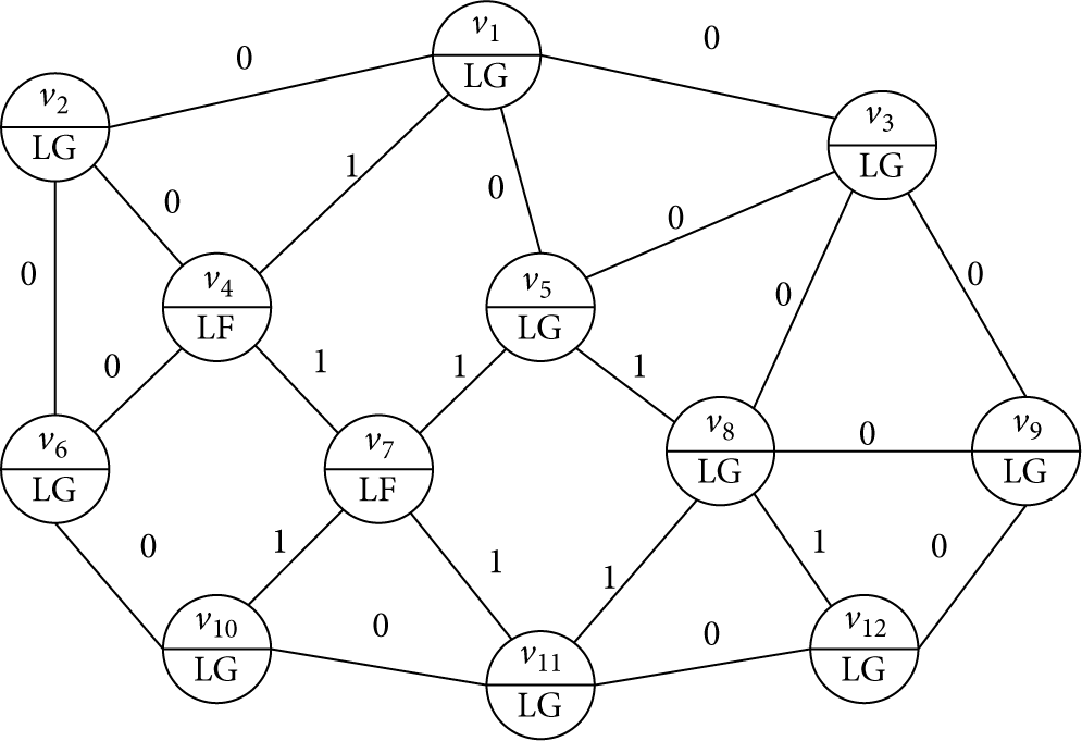
Illustration of a fault detection algorithm for a wireless sensor network.
The results of performing the detection algorithm are shown in Table 1. The final detected states and the preliminary states of the nodes were consistent except for nodes
Detection process and results for the algorithm used on the wireless sensor network shown in Figure 2.
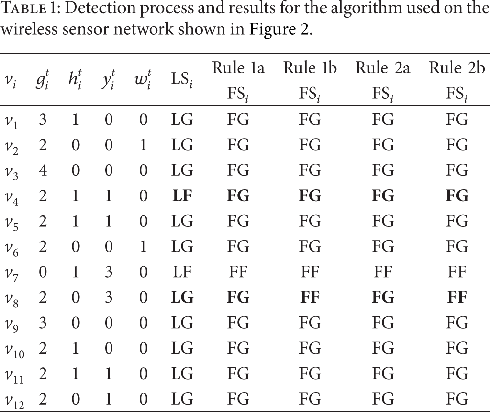
Node
5. Performance Evaluation
The proposed STCFD depends on a number of parameters (the threshold values
5.1. Real-World Dataset from the Intel Berkeley Research Laboratory
The Intel Berkeley Research Laboratory (IBRL) dataset was used as a real world dataset for testing the proposed model. The data were collected from 54 Mica2Dot sensors that were deployed in the IBRL between 28 February and 5 April 2004. The position of each node in the deployment area is shown in Figure 3. The Mica2Dot sensors had weather boards and collected time-stamped topology information and humidity, temperature, light, and voltage values once every 31 s. The data were collected using a TinyDB in-network query processing system, which was built in the TinyOS platform. The IBRL dataset included a log of about 2.3 million readings from these sensors [20].

Sensor nodes deployed to collect the Intel Berkeley Research Laboratory dataset.
The temperature dataset for two consecutive days (from 00:00 to 24:00), 28 February and 29 February, was selected from the experimental data. The data from 28 February were used to estimate the SARIMA model parameters. The fault detection methods were evaluated using the data from 29 February. The transmission range of the nodes was chosen to ensure that the sensors had different average numbers of neighbours in the simulation runs. An example of the network topology is shown in Figure 4. The relationships between the transmission range
Relationships between the transmission range


An illustration of the network topology when
5.2. Data Preprocessing
The proposed STCFD is a distributed parallel algorithm, and it requires time synchronized data to be input. However, different nodes cannot collect data at the same time because the Mica2Dot sensor would miss some of the data packages. The IBRL dataset could not therefore be directly used in the STCFD, and we had to preprocess the data before it was input to the algorithm. We used a smoothing window to modify the original data to keep the gathered data synchronized. The smoothing window outputs the average value, giving samples at specified time intervals. The smoothing window size could be set at 10, 20, 30, or 60 min, as required.
The raw IBRL data are shown in Figure 5(a), and the data processed using smoothing window of 30 min is shown in Figure 5(b). The smoothing window was 30 min in the analysis described below. Each sensor node could acquire 48 time series samples between 00:00 and 24:00 on 29 February.
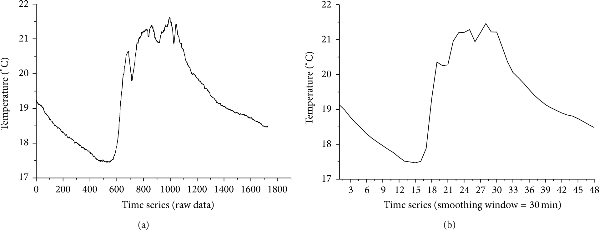
(a) Raw data for node 1 from 00:00 to 24:00 on 29 February and (b) time series samples for node 1 from 00:00 to 24:00 on 29 February produced using a smoothing window of 30 min.
Analysing the 48 samples from each sensor node on 28 February easily showed that the samples satisfied AR(2), and the desired prediction data were easily obtained. For example, the sampling data and their forecasts for node 1 on 29 February are shown in Figure 6.

Sampling data and forecasts for node 1 on 29 February (using a smoothing window of 30 min).
Some artificial anomalies with slightly deviating statistical characteristics were inserted to allow the anomaly detection models to be evaluated using these samples. The maximum temperature in the 2592 samples from 54 nodes on 29 February was 23.0°C and the minimum was 14.9°C. Taking the maximum difference between neighbouring sensors into account, random measured values were generated using the temperature ranges (0, 12) and (26, 40) as faults, and they were inserted into the normal dataset.
5.3. Experimental Results
The DR and FPR values produced in simulations using different parameters and rules were compared. We assumed that the network was available when the number of faulty nodes was less than half the total number of nodes in the WSN. Sensors were randomly chosen to be faulty, and the number of faulty sensors was set in the range 1–27. We will now discuss the effects on the algorithm of using different parameters in the experiments described below. Each experimental result was the average of 30 independent runs.
5.3.1. Experiment I: Variable
,
, and
m
In experiment I we determined the faulty node detection rate and false alarm rate using different
As can be seen in Figures 7 and 8, increasing the number of faulty nodes caused the DR using Rule 1a and Rule 1b to decrease gradually. The DR using Rule 1a was higher when
(a) Detection rate (DR) for algorithm Rule 1a when

(a) Detection rate (DR) for algorithm Rule 1b when
In Figure 8, larger
It can be seen from Figures 9 and 10 that the DR using Rule 2a and Rule 2b almost stayed the same as the number of faulty nodes was changed. However, the DR using Rule 2a was affected by the
(a) Detection rate (DR) for algorithm Rule 2a when

(a) Detection rate (DR) for algorithm Rule 2b when
The
Two main conclusions were drawn from Experiment I. (1)
5.3.2. Experiment II: Variable
,
, and
m
Experiment II gave the faulty node detection rate and false alarm rate using different
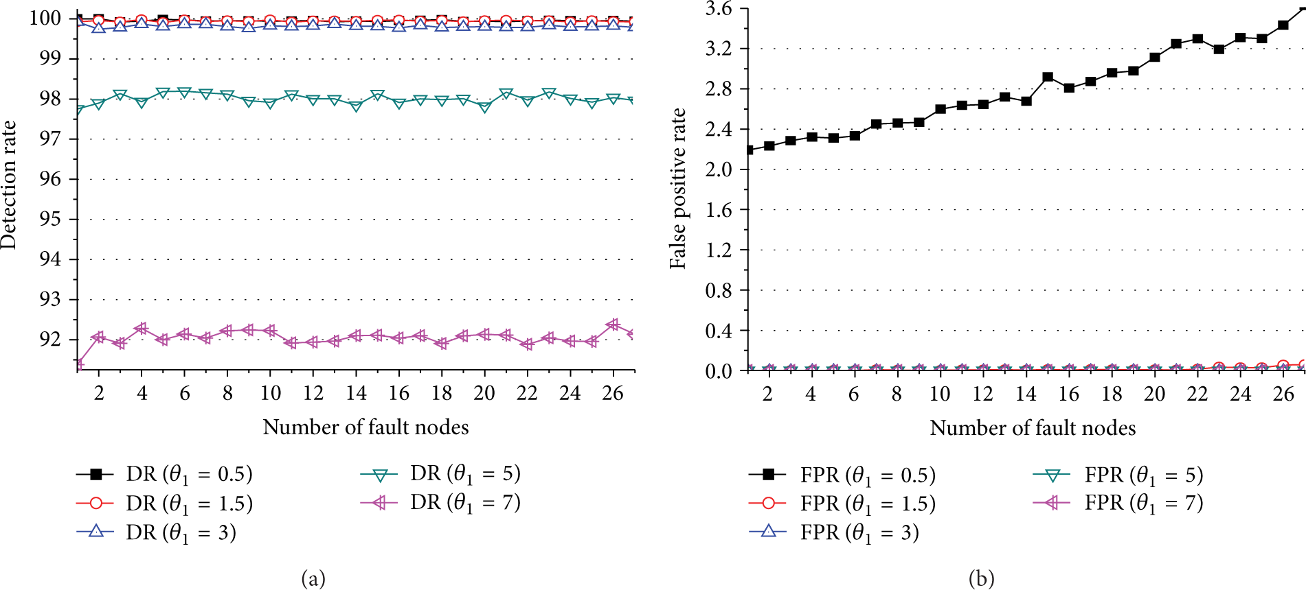
It can be seen from Figures 11 and 12 that the DRs obtained using Rule 1a and Rule 1b were similar. The

(a) Detection rate (DR) for algorithm Rule 1a when

(a) Detection rate (DR) for algorithm Rule 1b when
The DR using Rule 1a was higher when
The best
The effects on the DR and FPR using Rule 2a and Rule 2b are clearly shown in Figures 13 and 14. Smaller

(a) Detection rate (DR) for algorithm Rule 2a when

(a) Detection rate (DR) for algorithm Rule 2b when
Two main conclusions were drawn from Experiment II. (1) The best
5.3.3. Experiment III: Variable
,
, and
The faulty node detection accuracies achieved using Rule 1a, Rule 1b, Rule 2a, and Rule 2b and the numbers of faulty nodes for different neighbours are shown in Figures 15 and 16.

(a) Detection rate (DR) and false positive rate (FPR) for algorithm Rule 1a when

(a) Detection rate (DR) and false positive rate (FPR) for algorithm Rule 2a when
Increasing
The DRs using Rule 2a and Rule 2b were almost independent of the average number of neighbours (Figure 16). Increasing the average number of neighbours caused the FPRs using Rule 2a and Rule 2b to decrease, but the FPRs increased as the number of faulty nodes increased. Even when half of the total number of sensors were faulty the DRs using Rule 2a and Rule 2b were still about 99.95%. The FPR using Rule 2a was 0.13% when
In brief, Experiment III showed that increasing the number of neighbours may improve the detection performances of algorithm Rule 1a, Rule 1b, Rule 2a, and Rule 2b.
5.3.4. Experiment IV: Comparing the Accuracies of Detection Achieved Using Different Algorithms
In the following experiments we compared the detection performances of our STCFD, a single time series model (STM) [18], and a distributed fault detection (DFD) algorithm [11].
(1) STCFD and STM. We used two scenarios to compare the performances of the STCFD and STM. (1)
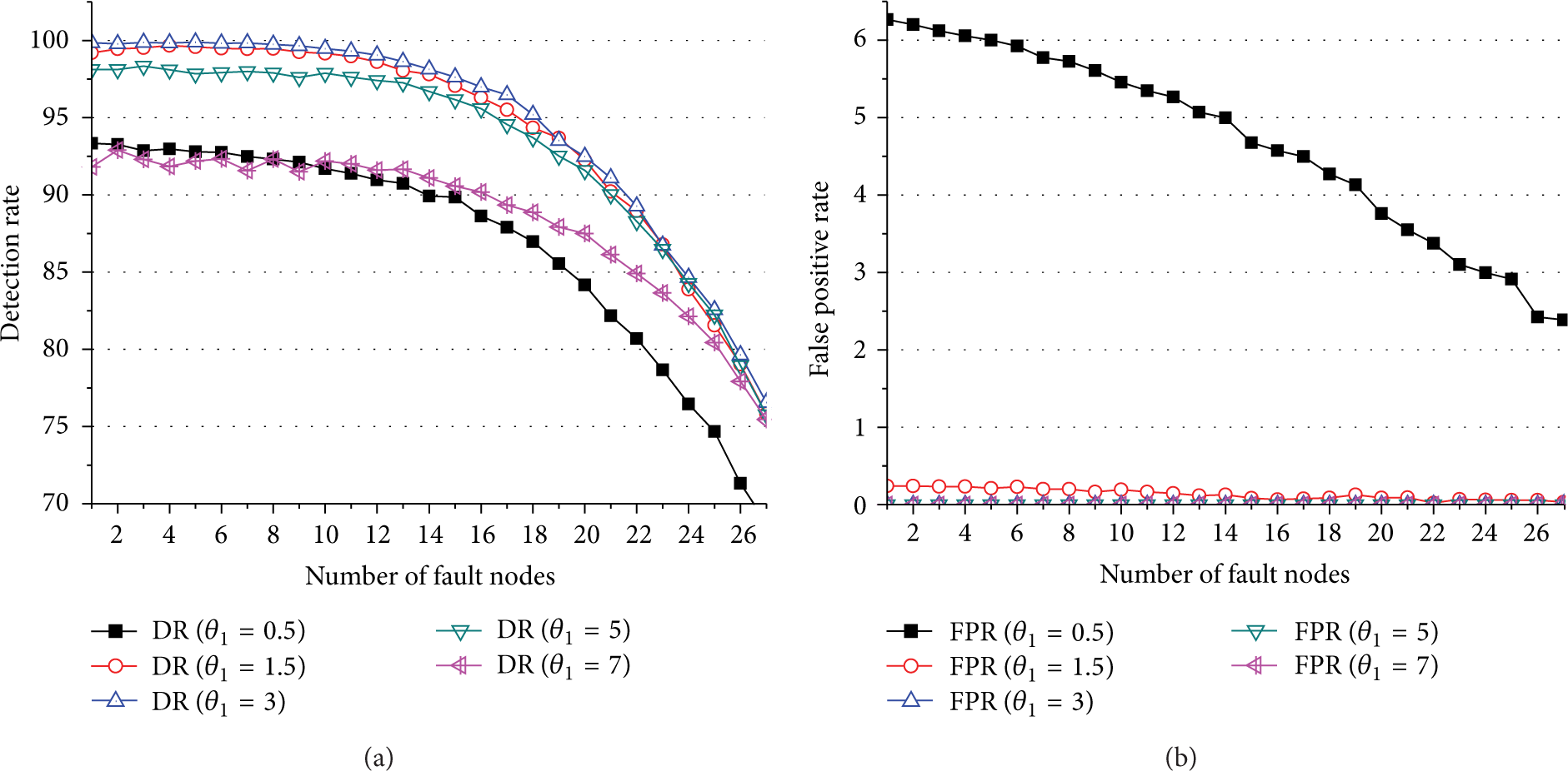
The STM DR was about 100% and the FPR remained at about 8%, and neither was affected by the number of faulty nodes (Figure 17). Increasing the number of failed nodes caused the DRs and FPRs using Rule 1a and Rule 1b to decrease nonlinearly (Figure 17(a)). The DRs decreased from about 93% to about 70%, the FPR using Rule 1a decreased from about 6.27% to 2.39%, and the FPR using Rule 1b decreased from about 7.68% to 2.56%. The DRs using Rule 2a and Rule 2b were about 99.95% and were not related to the number of faulty nodes (Figure 17(b)), the FPR using Rule 2a increased from about 2.19% to 3.63%, and the FPR using Rule 2b increased from about 2.47% to 4.96%, and both of the FPRs were less than the STM FPR (8%). Rule 1a and Rule 1b gave lower false alarm rates than the STM, but at the expense of a lower detection rate. Rule 2a and Rule 2b obviously gave lower false alarm rates than the other methods and maintained a high detection rate that was equivalent to that achieved using the STM.

(a) Detection rate (DR) and false positive rate (FPR) for the single time series model (STM) and the algorithm Rule 1a and Rule 1b when
It can be seen from Figure 18 that the FPR using the STM was only 0% but the DR using the STM was about 98%. The DR using Rule 1a decreased from 98.11% to 75.76%, and the DR using Rule 2a was about 98%. Neither Rule 1a nor Rule 2a improved the detection accuracy because their DRs were not higher than the DR achieved using the STM.

(a) Detection rate (DR) and false positive rate (FPR) for the single time series model (STM) and the algorithm Rule 1a and Rule 1b when
The DR using Rule 2b was about 99.95%, which was higher than was achieved using the STM (2%). The FPR using Rule 2b only increased from 0.18% to 1.62%. When the number of faults was <16, the DR using Rule 1b was higher than was achieved using the STM (1.90%–0.03%), and the corresponding FPR was also higher than was achieved using the STM (0.18%–0.01%). These results imply that the FPRs were increased less than the DRs using algorithm Rule 2b and Rule 1b relative to using the STM, so Rule 2b and Rule 1b gave better detection performances than the STM. Experiment IV showed that we can produce an STCFD rule that will increase the detection rate or decrease the false positive rate under different conditions, to improve the detection accuracy over that achieved using the STM.
(2) STCFD and DFD. Different types of parameters are available, so it is difficult to compare the different algorithms exactly. We chose relatively moderate values for appropriate parameters so that we could compare the STCFD and DFD algorithms in general terms. We used
The DRs and FPRs achieved using the STCFD and DFD methods plotted against the numbers of faulty sensors are shown in Figure 19. The DR using DFD, Rule 1a, and Rule 1b decreased as the number of faulty nodes increased. When the number of faulty nodes was <12, the DR using the DFD was >99.0% and was slightly higher than or at least equal to the DRs achieved using Rule 1a and Rule 1b. When the number of faulty nodes increased from 12 to 24, the DR using the DFD decreased sharply until it fell below 70%, but the DRs using Rule 1a and Rule 1b only decreased to about 84%. Some sensors may not have enough neighbours for a correct and complete analysis to be achieved, so faulty sensors were not diagnosed as faulty using the DFD. Increasing the number of faulty sensors caused the FPR using the DFD to increase from 0.65% to 2.4% and then to decrease to 1.62%.

(a) Detection rate (DR) and false positive rate (FPR) for the distributed fault detection method (DFD) and the algorithm Rule 1a and Rule 1b and (b) DR and FPR for the DFD and the algorithm Rule 2a and Rule 2b.
The DRs and FPRs using Rule 2a and Rule 2b were higher than the DR using the DFD. The DRs using Rule 2a and Rule 2b were still about 99.95% when 27 sensors were faulty. Furthermore, the FPR using Rule 2a increased from 0% to 0.06% and the FPR using Rule 2b increased from 0.22% to 1.20%. It is clear that our STCFD gives a better fault detection accuracy than does the DFD, especially when the number of faulty nodes is higher than in the target network.
5.4. Complexity Analysis
There are usually strict constraints on resources when WSN algorithms are performed, and this is a significant difference from other scenarios in which such algorithms are used. A very accurate but resource-hungry method is hardly applicable to WSNs. We analysed the complexity of the STCFD method, including the communication, computation, and memory demands.
The computational complexity was found to depend mainly on the time series model used to calculate
6. Conclusions
In this paper we present a method for detecting distributed faults in coordinate-free WSNs. The method is based on spatial and temporal correlations in WSN data. Firstly, we used a time series analysis method to determine the preliminary detection state for each node. Secondly, we used spatial correlations of adjacent nodes to obtain a comparison test result
Experimental results obtained using a real database gave the following results. (1) The four rules in our algorithm give different detection accuracies. Rule 1a and Rule 1b use the inequality
Our algorithm is promising, and we intend to extend it to see how it behaves in extremely large deployments. In further research and simulations, we will use our proposed algorithms in real situations. We will focus on the following four aspects: (1) using more complex data structures, with seasonal, cyclical, and other trends, (2) inserting different fault types (short faults, noise faults, and constant faults) or fault intervals into real data for detection tests, (3) using different SARIMA values for the forecast for each node, rather than uniform values as used in the experiments described above, and (4) optimizing the analysis process to decrease the complexity of the algorithm.
Footnotes
Conflict of Interests
The authors declare that there is no conflict of interests regarding the publication of this paper.
Acknowledgments
The work was supported by the key National Natural Science Foundation of China under Grant 91118005, the key Projects in the National Science & Technology Pillar Program during the Twelfth Five-year Plan Period under Grant 2011BAJ03B13, the Fundamental Research Funds for the Central Universities of China under Grant 106112014 CDJZR098801. The real-world dataset was provided by Intel Berkeley Research lab, thanks for their hard work.