Achieving Distributed Consensus in UWB Sensor Networks: A Low Sampling Rate Scheme with Quantized Measurements

Abstract

Distributed consensus in sensor networks has received great attention in the last few years. Most of the research activity has been devoted to study the sensor interactions that allow the convergence of distributed consensus algorithms toward a globally optimal decision. On the other hand, the problem of designing an appropriate radio interface enabling such interactions has received little attention in the literature. Motivated by the above consideration, in this work an ultrawideband sensor network is considered and a physical layer scheme is designed, which allows the active sensors to achieve consensus in a distributed manner without the need of any admission protocol. We focus on the class of the so-called quantized distributed consensus algorithms in which the local measurements or current states of each sensor belong to a finite set. Particular attention is devoted to address the practical implementation issues as well as to the development of a receiver architecture with the same performance of existing alternatives based on an all-digital implementation but with a much lower sampling frequency on the order of MHz instead of GHz.

1. Introduction

A sensor network denotes a collection of spatially distributed radio transceivers equipped with sensors that communicate through wireless links without the need of any fixed infrastructure (see [1, 2] and references therein). The absence of any centralized control mechanism makes sensor networks particularly suited for a large number of civil and industrial applications including surveillance, healthcare, factory-automation, and in-vehicle sensing [3].

Although their potential benefits in all the above applications are widely recognized, the implementation of sensor networks poses several technical challenges, which are substantially different from those of conventional communication systems. One of the primary interests is represented by the need to conjugate the relative unreliability of a single sensor (due to its limited complexity and energy availability) with the high reliability required to the whole network. For this reason, an intense research activity has been recently devoted to designing algorithms by which all the active sensors may reach an agreement on certain quantities of interest in a distributed manner. This problem is known as consensus in the literature and has a long standing tradition in computer science (see, e.g., [4–6] and references therein for a comprehensive overview of the problem). In sensor networks, particular attention has been given to the characterization of the conditions for achieving consensus (see, e.g., [7, 8]) while only few works deal with the problem of designing appropriate radio interfaces that allow achieving consensus. Motivated by the above consideration, in this work, we concentrate on the physical layer and assume that the active sensors interact directly in a peer-to-peer fashion without employing any admission protocol and using ultrawideband with impulse radio (UWB) as a common air interface [9]. This technology is nowadays considered as one of the most promising candidate for supporting emerging sensor network applications [10]. In UWB systems the information is conveyed by low-power ultrashort pulses whose bandwidth is on the order of a few GHz. The low transmit power facilitates the coexistence of UWB devices with different types of wireless services (a situation that is likely to occur with sensor networks) while the short duration provides the system with high-time resolution, which improves ranging accuracy (particularly useful for a large variety of sensor network applications such as control and monitoring). In addition, UWB systems provide the possibility to realize transceiver architectures in a low-energy consumption and integrated fashion as it is desirable in sensor networks in order to reduce the size and increase the battery life of the wireless devices. All these features make the UWB technology particularly appealing for the aforementioned applications and justify its adoption as a physical layer technique in the IEEE 802.15.4a standard [11].

A first attempt to design a radio interface for the practical implementation of a distributed consensus algorithm was originally presented by Akaiwa et al. in [12] for interbase station synchronization in microcellular systems and later extended to intervehicle communications by Sourour and Nakagawa in [13]. Such a scheme makes use of a pulse-position modulation (PPM) technique to transmit the current state of each vehicle. This information is then recovered at the receiver measuring the amplitudes and relative time of arrivals of the signal peaks exceeding a properly designed threshold. Unfortunately, the above solution provides good performance only in those applications in which the channel can be modeled as Gaussian. Obviously, this model does not hold true in both indoor and outdoor UWB transmissions in which the sensor network covers a nonnegligible area and each transmitted pulse propagates through a large number of distinct paths and it is seen by the receiver as the superposition of multiple echoes, each characterized by a different shape and a random position in the time scale. A scheme that is robust to multipath propagation was discussed by Simeone and Spagnolini in [14]. Here, the authors propose a barycenter-based time-detector whose aim is to estimate a convex combination of the arrival times of all the received pulses rather than explicitly estimating only those associated with the largest peaks. A similar approach is followed by Pescosolido et al. in [15] while other solutions can be found in [15, 16]. Differently from [14], however, the result in [15] is achieved by application of an alternative solution based on a double integration of the received signal. As discussed later, the main drawback of these two schemes is that they require “all-digital” receivers. Albeit possible in principle, the realization of an “all-digital” receiver in UWB sensor networks is challenging. The main problem is represented by the need of using analog-to-digital converters (ADCs) operating in the multi-GHz range and characterized by both low-power consumption and high-moderate bit resolution. Unfortunately, all these requirements cannot be easily satisfied with current technology. For example, the amount of power required by a common flash ADC increases linearly with the sampling rate and exponentially with the bit resolution [17]. Vice versa, the so called successive approximation register ADCs can be employed only in those applications characterized by low sampling rate and high bit resolution [18]. In summary, an “all-digital” implementation of the UWB receiver in sensor networks appears unfeasible.

Motivated by the above discussion, in this work, a simple iterative distributed algorithm is considered and a physical layer scheme is proposed that allows achieving consensus on a common parameter of interest with affordable complexity. In particular, we consider a collection of sensors connected by wireless links operating in a half-duplex manner and composed of the following basic components. A transducer that is used to monitor the physical parameter of interest and a dynamical system whose state evolves in time according to the local measurements and the states of nearby nodes. Finally, a radio interface that is used to transmit the state of the dynamical system and receive those of nearby sensors. We consider the class of the so-called quantized distributed consensus algorithms in which the local measurements or current states of each sensor belong to a finite set (see, e.g., [19–21] and references therein). In particular, the effective local measurement of each sensor is first quantized on a specified number of levels and then launched over the physical channel using an UWB signal with PPM. Each sensor updates its current state according to the iterative algorithm on the basis of the signals received from its neighbors. In particular, the state increment is computed resorting to the barycenter-based scheme illustrated in [14]. The latter is first revised to be applied to the system under investigation and then extended as follows. First, we discuss the conditions under which its operation is guaranteed in UWB transmissions operating over frequency-selective channels. Second, we propose a simple alternative solution, which operates at a much lower sampling frequency on the order of MHz. This translates into a receiver architecture of reduced complexity and low-energy consumption in accordance with the implementation constraints posed by UWB sensor networks. Third, we assume that the analog estimate of the state increment obtained with such a reduced complexity solution is processed by an $N_b$ -bit quantizer before being passed to the iterative algorithm. Then, we discuss the crucial issue of the system parameter setting, which is required to ensure the convergence of the consensus algorithm. For completeness, we return also to the method proposed in [15] and show that it is mathematically equivalent to [14] except for a normalization factor, which depends on the energy of the received signal. Numerical results are used to assess the effectiveness of the proposed scheme and to make comparisons with the existing alternatives. To this end, an UWB scenario inspired by the IEEE 802.15.4a standard is adopted. These results give a useful guidance on how to improve the performance of the investigated solution in practical applications and on how all the considered aspects interact to each other. To the best of our knowledge, this is the first time that such an analysis is carried out in a practical simulation setup for UWB sensor networks.

In summary, the major contributions of this work can be summarised as follows.

• (a)

It proposes a simple receiver architecture which has a much lower complexity compared to existing alternatives.

(b)

It provides a sufficiently detailed analysis of the communication and implementation problems arising in sensor networks using UWB technologies. This may represent in our opinion a useful guidance for system developers that aim at setting the system parameters of practical applications.

(c)

Some critical implementation issues arising in practical applications are discussed such as (i) the development of a receiver architecture of reduced complexity and low-energy consumption in accordance with the implementation constraints posed by UWB sensors; (ii) the design of a suitable threshold able to remove the extra noise with ensuing enhancement of the system performance; (iii) the study of the impact of the number of bits used by the quantizer on the system performance.

(d)

The performance of the proposed physical layer scheme is assessed and validated using different channel models inspired to the IEEE 802.15.4a standard.

All this may serve as an incentive to the research community for further investigations since most of the problems addressed in this work have been completely neglected so far.

The rest of the paper is organized as follows. Next section formulates the problem and describes the system under investigation. In Section 3 the barycenter-based scheme is first revised and then modified to enable its physical implementation. Some useful remarks are discussed in Section 4. Numerical results are presented in Section 5 while some conclusions are drawn in Section 6.

2. Problem Statement and System Description

2.1. Problem Statement

We consider a collection of M sensors and we call $\theta \in ℝ$ the physical parameter to be estimated. Thus, denoting by ${\chi }_k^{(\mathrm{1})}$ the initial estimate of the kth sensor, we may write

$$\begin{array}{cc}& {\chi }_k^{\left(\mathrm{1}\right)}=\theta +{\varsigma }_k\hspace{1em}\text{for}\hspace{0.17em}k=\mathrm{1,2},\dots ,M,\end{array}$$

(1)

where ${\varsigma }_k$ is a disturbance term modeled as a zero mean random variable.

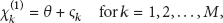
As mentioned before, we consider the class of quantized consensus algorithms in which the initial estimate ${\chi }_k^{(\mathrm{1})}$ takes values in the finite range $({\chi }_{\min },{\chi }_{\max })$ and is mapped into the finite set 𝒵 of cardinality $\left|𝒵\right|$ according to the following rule:

$$\begin{array}{cc}& z_k^{\left(\mathrm{1}\right)}=\lfloor \frac{{\chi }_k^{\left(\mathrm{1}\right)}}{I_z}\rceil -z_{\min },\end{array}$$

(2)

where $\lfloor c\rceil$ indicates the integer closest to c and $I_z$ is a design parameter whose dimension is dictated by the type of physical parameter to be estimated while $z_{\min }$ is given by $z_{\min }={\chi }_{\min }/I_z$ (for simplicity, we assume that ${\chi }_{\min }$ is a multiple of $I_z$ ). It is worth observing that $I_z$ plays a key role on the estimation accuracy of the consensus algorithm as it controls the quantization error affecting the exchanged information. Albeit its practical interest, it is not considered in this work since it depends on the specific application for which the sensor network is employed. Only a comment will be provided in Section 5 to show how its effects can be taken into account.

The information associated with the initial states is exchanged among the active sensors and used by the distributed algorithm to eventually drive the network toward a consensus from which an estimate of θ is eventually computed. Since we consider low mobility applications in which the propagation channel changes slowly compared to the convergence time of the iterative algorithm (as shown in Section 5, the convergence time of the proposed algorithm is relatively small, i.e., on the order of few microseconds), the connection links are assumed to maintain constant over the time interval required by the consensus algorithm to converge. In the above circumstances, the dynamic of the iterative algorithm can be mathematically described by the following recursion:

$$\begin{array}{cc}& z_k^{\left(n+\mathrm{1}\right)}=z_k^{\left(n\right)}+\lfloor \mu \left(n\right)e_k^{\left(n\right)}\rceil \hspace{1em}\text{for}\hspace{0.17em}\hspace{0.17em}n=\mathrm{1,2},\dots ,\end{array}$$

(3)

where $z_k^{(n)}$ denotes the estimate or state of the kth sensor at the nth iteration and $\mu (n)$ is a nonnegative design parameter (known as step size) that controls the convergence properties of the iterative algorithm while

$$\begin{array}{cc}& e_k^{\left(n\right)}={\displaystyle \sum }_{i\in {ℳ}_k}‍{\rho }_{k,i}\left(z_i^{\left(n\right)}-z_k^{\left(n\right)}\right)\end{array}$$

(4)

is the corresponding state increment. In the above equation, ${ℳ}_k$ denotes the set that contains the indexes of the neighbors communicating with the kth sensor while the quantities $\{{\rho }_{k,i}\}$ are the real-valued nonnegative coupling coefficients accounting for the interactions among the connected sensors.

In Section 5, we will show that an appropriate setting of the system parameters allows the iterative procedure in (3) to converge to the following asymptotic result:

$$\begin{array}{cc}& \underset{n\to \infty }{\lim }{z}_k^{\left(n\right)}=\lfloor \frac{\mathrm{1}}{M}{\displaystyle \sum }_{i=\mathrm{1}}^M‍z_i^{\left(\mathrm{1}\right)}\phantom{{\displaystyle \sum }_{i=\mathrm{1}}^M‍}\rceil .\end{array}$$

(5)

From (3) and (4), we see that the current state $z_k^{(n)}$ can be updated only if we assume that the generic kth sensor has knowledge of the states $\{z_i^{(n)};i\ne k\}$ of its neighbors. Obviously, this assumption is not valid in practical applications. For this reason, an UWB-based radio interface to exchange this information is described in the next.

2.2. System Description

Similar to [14, 15], we consider a frequency-synchronized network in which all the active sensors have a clock that evolves in time with a common period of duration T. As in [14, 15], we also assume that the consensus phase is preceded by an acquisition procedure that allows the sensors to align the time reference scales.

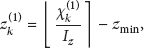
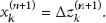
Each sensor transmits its own state using an UWB signal with PPM. For this purpose, the state variable $z_k^{(n)}$ for any $k=\mathrm{1,2},\dots ,M$ and $n=\mathrm{0,1},\dots$ is mapped prior to transmission onto its corresponding timing delay as follows:

$$\begin{array}{cc}& x_k^{\left(n\right)}=\Delta z_k^{\left(n\right)},\end{array}$$

(6)

where Δ is a system parameter designed later. The quantity $x_k^{(n)}$ is then used to modulate the position of ultrashort pulses whose duration is on the order of a few nanoseconds.

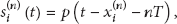
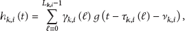
The signal transmitted by the ith sensor during the nth symbol takes the form illustrated in Figure 1 and is mathematically described by

$$\begin{array}{cc}& s_i^{\left(n\right)}\left(t\right)=p\left(t-x_i^{\left(n\right)}-nT\right),\end{array}$$

(7)

where $p(t)$ denotes an ultrashort pulse. The transmitted signals propagate through different channels and undergo multipath propagation.

Figure 1

Illustration of the UWB signal with PPM.

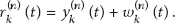
At each sensor, the incoming waveforms are implicitly recombined by the receive antenna and fed to a receive filter, which has a rectangular transfer function with bandwidth B sufficiently large to pass the signal pulses undistorted. As discussed later, if the symbol duration T is properly chosen, the signal received at the kth sensor during the nth symbol can be mathematically written as

$$\begin{array}{cc}& r_k^{\left(n\right)}\left(t\right)=\{\begin{array}{cc}{y}_k^{\left(n\right)}\left(t\right)+w_k^{\left(n\right)}\left(t\right)\hfill & \text{if}\hspace{0.17em}{s}_k^{\left(n\right)}\left(t\right)=\mathrm{0}\hfill \\ 0\hfill & \text{if}\hspace{0.17em}{s}_k^{\left(n\right)}\left(t\right)\ne \mathrm{0},\hfill \end{array}\end{array}$$

(8)

where we have taken into account that each sensor operates in an half-duplex manner meaning that it cannot receive the signal during the time in which it is transmitting. In the above equation, $w_k^{(n)}(t)$ is the thermal noise modeled as a Gaussian random process with zero mean and two-sided power spectral density $N_{\mathrm{0}}/\mathrm{2}$ while $y_k^{(n)}(t)$ takes the form

$$\begin{array}{cc}& y_k^{\left(n\right)}\left(t\right)={\displaystyle \sum }_{i\in {ℳ}_k}‍h_{k,i}\left(t-x_i^{\left(n\right)}-nT\right).\end{array}$$

(9)

In addition, $h_{k,i}(t)$ denotes the overall channel impulse response between the kth and ith sensor and is given by

$$\begin{array}{cc}& h_{k,i}\left(t\right)={\displaystyle \sum }_{\ell =\mathrm{0}}^{L_{k,i}-\mathrm{1}}‍{\gamma }_{k,i}\left(\ell \right)g\left(t-{\tau }_{k,i}\left(\ell \right)-{\nu }_{k,i}\right),\end{array}$$

(10)

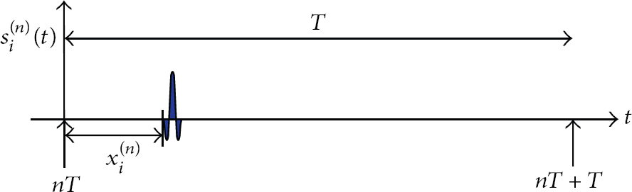
where $L_{k,i}$ denotes the number of distinct paths while $g(t)$ is obtained as the convolution of the transmit and the receive filters. Finally, ${\gamma }_{k,i}(\ell )$ is the gain of the ℓth path and ${\tau }_{k,i}(\ell )$ is its corresponding delay while the quantity ${\nu }_{k,i}$ stands for a possible misalignment, due to the timing errors of the initial synchronization phase, between the time reference scales of user k and i (see Figure 2).

Figure 2

Illustration of the relationship between the signal transmitted by sensor i and the corresponding signal received by sensor k.

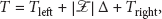
We are now left with the problem of designing the symbol duration T. The latter must be chosen long enough so as to accommodate the transmission intervals, the channel delay spreads, and the possible timing misalignments among the active sensors. Mathematically, this amounts to setting

$$\begin{array}{cc}& T=T_{\text{left}}+\left|𝒵\right|\Delta +T_{\text{right}},\end{array}$$

(11)

where $T_{\text{left}}$ and $T_{\text{right}}$ are design parameters that depend on the channel characteristics and the residual timing offsets. In particular, the quantity $T_{\text{left}}$ accounts for the maximum leftward timing shift among the signals received from all the sensors and is given by

$$\begin{array}{cc}& T_{\text{left}}={\nu }_{\max }-{\nu }_{\min }-{\tau }_{\min },\end{array}$$

(12)

where ${\tau }_{\min }={\min }_{k,i,\ell }\{{\tau }_{k,i}(\ell )\}$ while ${\nu }_{\max }$ and ${\nu }_{\min }$ are, respectively, defined as ${\nu }_{\max }={\max }_{k,i}\{{\nu }_{k,i}\}$ and ${\nu }_{\min }={\min }_{k,i}\{{\nu }_{k,i}\}$ . On the other hand, $T_{\text{right}}$ denotes the maximum rightward timing shift induced by the channels of the active sensors and takes the form

$$\begin{array}{cc}& T_{\text{right}}={\nu }_{\max }-{\nu }_{\min }+{\tau }_{\max }\end{array}$$

(13)

with ${\tau }_{\max }={\max }_{k,i,\ell }\{{\tau }_{k,i}(\ell )\}$ .

3. A Practical State Increment Estimator

In this section, we first adapt the method illustrated in [14] to the system under investigation and then we discuss its implementation issues.

3.1. Barycenter-Based Estimation

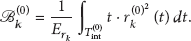
Without loss of generality, we concentrate on the signal received by the kth sensor during the nth interval and assume that $t=\mathrm{0}$ denotes the start of the considered interval in the kth time scale.

We start shifting leftward the received signal by a quantity $x_k^{(n)}$ . Next, we compute the barycenter of the resulting signal $r_k^{(n)}(t+x_k^{(n)})$ over the observation window of duration T and given by $T_{\mathrm{int}}^{(n)}=[nT-T_{\text{left}},nT+\left|𝒵\right|\Delta +T_{\text{right}}]$ . This produces

$$\begin{array}{cc}& {ℬ}_k^{\left(n\right)}=\frac{\mathrm{1}}{E_{r_k}^{\left(n\right)}}{{\displaystyle \int }}_{T_{\mathrm{int}}^{\left(n\right)}}‍t·r_k^{{\left(n\right)}^{\mathrm{2}}}\left(t+x_k^{\left(n\right)}\right)dt,\end{array}$$

(14)

where $E_{r_k}^{(n)}$ is the energy of $r_k^{(n)}(t)$ ; that is, $E_{r_k}^{(n)}={\int }_{T_{\mathrm{int}}^{(n)}}‍r_k^{(n{)}^{\mathrm{2}}}(t)dt$ .

We begin by observing that in UWB systems the time interval required to transmit the information signal $s_k^{(n)}(t)$ is usually a small fraction of the symbol duration T. Then, to ease the notation and to facilitate the mathematical computations, we may reasonably approximate (8) as follows:

$$\begin{array}{cc}& r_k^{\left(n\right)}\left(t\right)=y_k^{\left(n\right)}\left(t\right)+w_k^{\left(n\right)}\left(t\right).\end{array}$$

(15)

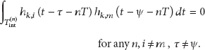
To proceed further, we assume that the signal-to-noise ratio (SNR) is relatively large so that the noise contribution can be neglected. Its effects will be taken into account later. Moreover, we assume that the signals received from different sensors do not overlap in time. This situation is sketched in Figure 3 and amounts to saying that the overall channel impulse responses satisfy the following condition:

$$\begin{array}{l}{{\displaystyle \int }}_{T_{\mathrm{int}}^{\left(n\right)}}‍h_{k,i}\left(t-\tau -nT\right)h_{k,m}\left(t-\psi -nT\right)dt=\mathrm{0}\hfill \\ \phantom{\text{hhhhhhhhhhhhhhhh}}\text{for}\hspace{0.17em}\text{any}\hspace{0.17em}n,i\ne m\hspace{0.17em},\hspace{0.17em}\tau \ne \psi .\hfill \end{array}$$

(16)

This assumption is not exactly satisfied in practical applications and it is adopted in this work only to simplify the analysis. Although not exactly satisfied and introduced only for analytical purposes, this assumption is quite reasonable in UWB systems thanks to the ultrashort nature of pulses and the heavy multipath behaviour of propagation channels that make the received signals highly uncorrelated [22]. This means that the proposed solutions will operate in a mismatched mode whose impact on the system performance will be evaluated by means of numerical results.

Figure 3

Illustration of the kth received signal.

In all the above circumstances (all of them will be removed in Section 5 where the performance of the proposed algorithm is evaluated numerically), we have that signal $r_k^{{(n)}^{\mathrm{2}}}(t+x_k^{(n)})$ in (14) takes the form

$$\begin{array}{cc}& r_k^{{\left(n\right)}^{\mathrm{2}}}\left(t+x_k^{\left(n\right)}\right)={\displaystyle \sum }_{i\in {ℳ}_k}‍h_{k,i}^{\mathrm{2}}\left(t-x_i^{\left(n\right)}+x_k^{\left(n\right)}-nT\right)\end{array}$$

(17)

while $E_{r_k}^{(n)}$ is given by

$$\begin{array}{cc}& E_{r_k}={\displaystyle \sum }_{i\in {ℳ}_k}‍E_{h_{k,i}},\end{array}$$

(18)

where the functional dependence from n has been omitted due to the above assumptions and we have defined $E_{h_{k,i}}$ the energy of $h_{k,i}(t)$ . Substituting (17) into (14) produces

$$\begin{array}{cc}& {ℬ}_k^{\left(n\right)}={\displaystyle \sum }_{i\in {ℳ}_k}\frac{\mathrm{1}}{E_{r_k}}{{\displaystyle \int }}_{T_{\mathrm{int}}^{\left(n\right)}}‍t·h_{k,i}^{\mathrm{2}}\left(t-x_i^{\left(n\right)}+x_k^{\left(n\right)}-nT\right)dt\end{array}$$

(19)

which can be rewritten in the following equivalent form

$$\begin{array}{cc}& {ℬ}_k^{\left(n\right)}={\displaystyle \sum }_{i\in {ℳ}_k}‍{\mathscr{H}}_{k,i}+{\displaystyle \sum }_{i\in {ℳ}_k}‍{\lambda }_{k,i}\left(x_i^{\left(n\right)}-x_k^{\left(n\right)}\right),\end{array}$$

(20)

where ${\lambda }_{k,i}$ is given by

$$\begin{array}{cc}& {\lambda }_{k,i}=\frac{E_{h_{k,i}}}{E_{r_k}}\end{array}$$

(21)

while ${\mathscr{H}}_{k,i}$ is defined as ${\mathscr{H}}_{k,i}=(\mathrm{1}/E_{r_k}){\int }_{T_{\mathrm{int}}^{(n)}}‍t·h_{k,i}^{\mathrm{2}}(t-nT)dt$ .

Dividing both sides of (20) by Δ, using (6), we obtain

$$\begin{array}{cc}& \frac{\mathrm{1}}{\Delta }{ℬ}_k^{\left(n\right)}=\frac{\mathrm{1}}{\Delta }{\displaystyle \sum }_{i\in {ℳ}_k}‍{\mathscr{H}}_{k,i}+{\displaystyle \sum }_{i\in {ℳ}_k}‍{\lambda }_{k,i}\left(z_i^{\left(n\right)}-z_k^{\left(n\right)}\right)\end{array}$$

(22)

from which it follows that ${ℬ}_k^{(n)}/\Delta$ is a biased estimate of the state increment given by (4) after replacing ${\rho }_{k,i}$ with ${\lambda }_{k,i}$ . To get rid of the bias term $(\mathrm{1}/\Delta ){\sum }_{i\in {ℳ}_k}‍{\mathscr{H}}_{k,i}$ , we follow the same line of reasoning illustrated in [15] and adopt a solution that was originally presented in [23]. In particular, it relies on the assumption that the transmission is preceded by a pilot symbol during which each sensor sets its own state to zero (i.e., $x_i^{(\mathrm{0})}=\mathrm{0}$ ) and transmits the following signal $s_i^{(\mathrm{0})}(t)=p(t)$ for $i=\mathrm{1,2},\dots ,M$ . In absence of noise, the kth received signal takes the form $r_k^{(\mathrm{0})}(t)={\sum }_{i\in {ℳ}_k}‍h_{k,i}(t)$ and is used to compute

$$\begin{array}{cc}& {ℬ}_k^{\left(\mathrm{0}\right)}=\frac{\mathrm{1}}{E_{r_k}}{{\displaystyle \int }}_{T_{\mathrm{int}}^{\left(\mathrm{0}\right)}}‍t·r_k^{{\left(\mathrm{0}\right)}^{\mathrm{2}}}\left(t\right)dt.\end{array}$$

(23)

Paralleling the same steps as before, we obtain

$$\begin{array}{cc}& {ℬ}_k^{\left(\mathrm{0}\right)}={\displaystyle \sum }_{i\in {ℳ}_k}‍{\mathscr{H}}_{k,i}.\end{array}$$

(24)

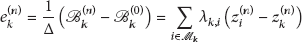
Once ${ℬ}_k^{(\mathrm{0})}$ is obtained, it can be exploited to compute the following quantity:

$$\begin{array}{cc}& e_k^{\left(n\right)}=\frac{\mathrm{1}}{\Delta }\left({ℬ}_k^{\left(n\right)}-{ℬ}_k^{\left(\mathrm{0}\right)}\right)={\displaystyle \sum }_{i\in {ℳ}_k}‍{\lambda }_{k,i}\left(z_i^{\left(n\right)}-z_k^{\left(n\right)}\right)\end{array}$$

(25)

which is used to update the state of the kth sensor according to (3). The timing offset $x_k^{(n+\mathrm{1})}$ is then obtained from $z_k^{(n+\mathrm{1})}$ as follows:

$$\begin{array}{cc}& x_k^{\left(n+\mathrm{1}\right)}=\Delta z_k^{\left(n+\mathrm{1}\right)}.\end{array}$$

(26)

The latter is eventually used to modulate the position of the UWB signal during the $n+\mathrm{1}$ time interval. In the sequel, the scheme based on (3) and (25)-(26) is referred to as the barycenter-based state increment estimator (BIE).

3.2. Implementation Issues

We begin by observing that the implementation of BIE needs the computation of (14) and (23). As depicted in Figure 4, evaluating these quantities requires to delay the signal at the output of the LPF by a quantity that in (14) depends on the index n. The resulting signal is passed through a square law device whose output is then multiplied by the continuous signal t and finally fed to an integrate and dump circuit with rate $\mathrm{1}/T$ . Although at a first glance all the above operations seem easily implementable, an accurate inspection reveals that among them there is one that may prevent the practical realization of BIE. This is represented by the tunable delay line, which must handle a wideband analog signal and must also be very accurate to guarantee the convergence of the iterative algorithm. Such an accurate and controlled device cannot be deployed with analog architectures unless expensive and cumbersome equipments are used. However, this is in sharp contrast to the low-cost and low-energy consumption requirements of UWB sensor networks [24]. A possible way out is to make use of an “all-digital” receiver [14], which operates directly on the samples of the signal at the LPF output taken at Nyquist rate. As mentioned previously, also this approach is not suited for sensor networks as it would require ADCs with sampling frequency of some GHz, which are too expensive and extremely energy consuming [25]. Motivated by the above arguments, in the sequel we propose an alternative solution, which dispenses from all the above impairments.

Figure 4

Block diagram of the receiver employing BIE.

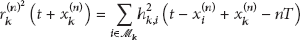
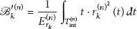
We start computing the barycenter of the received signals $r_k^{(n)}(t)$ . This produces

$$\begin{array}{cc}& {ℬ}_k^{\prime \left(n\right)}=\frac{\mathrm{1}}{E_{r_k}^{\left(n\right)}}{{\displaystyle \int }}_{T_{\mathrm{int}}^{\left(n\right)}}‍t·r_k^{{\left(n\right)}^{\mathrm{2}}}\left(t\right)dt\end{array}$$

(27)

from which using the same arguments of the previous section it follows that

$$\begin{array}{cc}& {ℬ}_k^{\prime \left(n\right)}={\displaystyle \sum }_{i\in {ℳ}_k}‍{\mathscr{H}}_{k,i}+{\displaystyle \sum }_{i\in {ℳ}_k}‍{\lambda }_{k,i}{x}_i^{\left(n\right)}.\end{array}$$

(28)

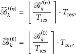
Then, we compute the following quantity:

$$\begin{array}{cc}& e_k^{\prime \left(n\right)}=\frac{\mathrm{1}}{\Delta }\left({ℬ}_k^{\prime \left(n\right)}-{ℬ}_k^{\left(\mathrm{0}\right)}-x_k^{\left(n\right)}\right).\end{array}$$

(29)

Substituting (24) and (28) into the above equation and observing that ${\sum }_{i\in {ℳ}_k}^{}{\lambda }_{k,i}=\mathrm{1}$ , we obtain

$$\begin{array}{cc}& e_k^{\prime \left(n\right)}={\displaystyle \sum }_{i\in {ℳ}_k}^{}{\lambda }_{k,i}\left(z_i^{\left(n\right)}-z_k^{\left(n\right)}\right)\end{array}$$

(30)

which represents an estimate of the state increment in the form given by (25).

From (24) and (27), we see that the computation of (29) does not require any delay line as it operates directly on the received signals. Indeed, the receiver block diagram of the proposed algorithm is that sketched in Figure 4 without the tunable delay line. The receiver architecture is now composed by two integrated and dump circuits, which operate at symbol rate of $\mathrm{1}/T$ and by a quantizer. Interestingly, $\mathrm{1}/T$ is much lower than the Nyquist rate since in the investigated system the Nyquist rate is on the order of some GHz while the symbol rate is on the order of some MHz.

We now observe that the state increment in (29) depends on ${ℬ}_k^{\prime (n)}$ and ${ℬ}_k^{(\mathrm{0})}$ . The latter are analog quantities that may take any value in the interval $(\mathrm{0},T)$ . In practical applications, however, only a quantized version of these variables can be passed to the consensus algorithm. For this reason, we assume that the receiver is equipped with a uniform $N_b$ -bit quantizer which produces

$$\begin{array}{cc}& {\widehat{ℬ}}_k^{\prime \left(n\right)}=\lfloor \frac{{ℬ}_k^{\prime \left(n\right)}}{T_{\text{res}}}\rceil ·T_{\text{res}},\\ {\widehat{ℬ}}_k^{\left(\mathrm{0}\right)}=\lfloor \frac{{ℬ}_k^{\left(\mathrm{0}\right)}}{T_{\text{res}}}\rceil ·T_{\text{res}},\end{array}$$

(31)

where $T_{\text{res}}=T/{\mathrm{2}}^{N_b}$ denotes the time-resolution of the quantizer. Replacing ${ℬ}_k^{\prime (n)}$ and ${ℬ}_k^{(\mathrm{0})}$ with ${\widehat{ℬ}}_k^{\prime (n)}$ and ${\widehat{ℬ}}_k^{(\mathrm{0})}$ into $e_k^{\prime (n)}$ in (29) yields

$$\begin{array}{cc}& {\widehat{e}}_k^{\prime \left(n\right)}=\frac{\mathrm{1}}{\Delta }\left({\widehat{ℬ}}_k^{\prime \left(n\right)}-{\widehat{ℬ}}_k^{\left(\mathrm{0}\right)}-x_k^{\left(n\right)}\right)\end{array}$$

(32)

which is eventually employed to update the state variable according to (3). The above scheme is called reduced-complexity BIE (RC-BIE) in the sequel.

4. Remarks

(i) Removing $E_{r_k}^{(n)}$ from the right-hand side of (14) produces

$$\begin{array}{cc}& {𝒫}_k^{\left(n\right)}={{\displaystyle \int }}_{T_{\mathrm{int}}^{\left(n\right)}}‍t·r_k^{{\left(n\right)}^{\mathrm{2}}}\left(t+x_k^{\left(n\right)}\right)dt\end{array}$$

(33)

from which using the rule of integration by parts we obtain

$$\begin{array}{cc}& {𝒫}_k^{\left(n\right)}=T·E_{r_k}^{\left(n\right)}-{{\displaystyle \int }}_{T_{\mathrm{int}}^{\left(n\right)}}‍{{\displaystyle \int }}_{\mathrm{0}}^t‍r_k^{(n{)}^{\mathrm{2}}}\left(t^{\prime }+x_k^{\left(n\right)}\right)d{t}^{\prime }dt.\end{array}$$

(34)

Letting $t_k^{\mathrm{\prime \prime }(n)}=-x_k^{(n)}-t^{\prime }$ and using standard manipulations yields

$$\begin{array}{cc}& {𝒫}_k^{\left(n\right)}=T·E_{r_k}^{\left(n\right)}+{{\displaystyle \int }}_{T_{\mathrm{int}}^{\left(n\right)}}‍u_k^{\left(n\right)}\left(t\right)dt\end{array}$$

(35)

with

$$\begin{array}{cc}& u_k^{\left(n\right)}\left(t\right)={{\displaystyle \int }}_{-x_k^{\left(n\right)}}^{-x_k^{\left(n\right)}+t}‍r_k^{{\left(n\right)}^{\mathrm{2}}}\left(-t_k^{\mathrm{\prime \prime }\left(n\right)}\right)d{t}_k^{\mathrm{\prime \prime }\left(n\right)}\end{array}$$

(36)

which are equivalent to the solution illustrated in [15]. As anticipated before, this means that the schemes in [14, 15] are substantially the same except for the normalization factor $E_{r_k}^{(n)}$ . Similar to [14], from (35) and (36), it follows that the method in [15] has a practical disadvantage: it requires to integrate the received signal over a sliding window of amplitude $[-x_k^{(n)},-x_k^{(n)}+t]$ . This operation can only be computed in digital form, thereby making it unsuited for practical applications. Following the same line of reasoning employed in the previous section for [14], a reduced complexity solution can be easily derived.

(ii) It is worth observing that the scheme presented in [15] does not employ any square device. This is due to the fact that the authors make use of pulses with unit area (this amounts to saying that ${\int }_{\mathrm{0}}^{{\tau }_g}‍g(t)dt=\mathrm{1}$ with ${\tau }_g$ being the duration of $g(t)$ ) rather than zero as assumed in this work. Under this assumption, the estimate of the error state increment can be computed as

$$\begin{array}{cc}& e_k^{\prime \left(n\right)}=\frac{\mathrm{1}}{\Delta }\left({𝒫}_k^{\prime \left(n\right)}-{𝒫}_k^{\prime \left(\mathrm{0}\right)}-E_{r_k}{x}_k^{\left(n\right)}\right),\end{array}$$

(37)

where ${𝒫}_k^{\prime (n)}$ and $E_{r_k}$ are now given by

$$\begin{array}{cc}& {𝒫}_k^{\prime \left(n\right)}={{\displaystyle \int }}_{T_{\mathrm{int}}^{\left(n\right)}}‍t·r_k^{\left(n\right)}\left(t\right)dt,\\ E_{r_k}={{\displaystyle \int }}_{T_{\mathrm{int}}^{\left(n\right)}}‍r_k^{\left(n\right)}\left(t\right)dt.\end{array}$$

(38)

Paralleling the same steps of before yields

$$\begin{array}{cc}& e_k^{\prime \left(n\right)}={\displaystyle \sum }_{i\in {ℳ}_k}‍{\lambda }_{k,i}\left(z_i^{\left(n\right)}-z_k^{\left(n\right)}\right),\end{array}$$

(39)

where ${\lambda }_{k,i}$ are now defined as follows:

$$\begin{array}{cc}& {\lambda }_{k,i}={{\displaystyle \int }}_{T_{\mathrm{int}}^{\left(n\right)}}‍h_{k,i}\left(t-nT\right)dt.\end{array}$$

(40)

Interestingly, the above results can be derived without imposing the condition (16) on the channel impulse responses of the active sensors. On the contrary, when a square law device is adopted the no interference condition must be fulfilled. This fact is particularly appealing as it would make the scheme based on (37)-(38) insensitive to the interference among the different channel impulse responses.

The main impairment of such a solution is that it would require bandpass communications since the direct current of a signal cannot be physically transmitted in baseband. Albeit feasible, this approach seems to be unsuited for practical UWB sensor networks as it would require the use of expensive and power consumption devices for the demodulation procedure.

(iii) As mentioned previously, in UWB systems, the signals transmitted by the active sensors propagate through different paths whose number is on the order of hundreds. This translates into a severe dispersion of the signal power at the receiving terminal. Then, it may happen that even for moderate values of SNRs the received signal is overwhelmed by the thermal noise, thereby preventing the application of all the investigated solutions. This situation is depicted in Figure 5, where the square of the received signal is shown for two different values of SNR assuming that the number of active sensors is $M=\mathrm{4}$ . As is seen, when the SNR is fixed to 10 dB the useful component cannot be distinguished from the received signal as it is completely overwhelmed by the thermal noise. A better situation is observed for an SNR of 20 dB. However, even for this favorable case it has been proven by computer simulations that all the investigated solutions fail. This fact can be explained observing that the observation window is equal to $T_{\mathrm{int}}^{(n)}$ . As depicted in Figure 5, $T_{\mathrm{int}}^{(n)}$ is much larger than the support of the useful component as it has been chosen so as to accommodate the channel delay spreads and all possible timing misalignments. Then, it may happen that, even for considerable values of SNR, the total amount of collected noise is too large to achieve acceptable performance. It is worth observing that these issues have been also partially discussed in [14] but only for a Gaussian channel in which they are less harmful for the following two reasons. First, all the transmitted power is concentrated in a single pulse that stands more easily over the noise. Second, in a Gaussian channel the observation window can be chosen shorter since the delay spread is limited to the duration of the transmitted pulses.

Figure 5

Illustration of the signal $r_k^{(n{)}^{\mathrm{2}}}(t)$ for different values of SNR when the number of active sensors is $M=\mathrm{4}$ .

A possible solution to contrast all the above problems is to make use of a properly designed threshold λ, which allows removing the extra noise. Omitting the time interval n for notational simplicity, this amounts to replacing $r_k^{\mathrm{2}}(t)$ with

$$\begin{array}{cc}& {\overline{r}}_k^{\mathrm{2}}\left(t\right)=\{\begin{array}{cc}{r}_k^{\mathrm{2}}\left(t\right)\hfill & \text{if}\hspace{0.17em}{r}_k^{\mathrm{2}}\left(t\right)\ge \lambda \hfill \\ 0\hfill & \text{if}\hspace{0.17em}{r}_k^{\mathrm{2}}\left(t\right)<\lambda .\hfill \end{array}\end{array}$$

(41)

To design λ, we compute the probability that the noise contribution is greater than λ within the observation window. Using (15) yields

$$\begin{array}{cc}& r_k^{\mathrm{2}}\left(t\right)=y_k^{\mathrm{2}}\left(t\right)+\mathrm{2}{y}_k\left(t\right)w_k\left(t\right)+w_k^{\mathrm{2}}\left(t\right)\end{array}$$

(42)

from which it follows that such a probability is given by

$$\begin{array}{cc}& P_{\text{th}}\left(\lambda \right)=\mathrm{2}·Q\left(\sqrt{\frac{\lambda }{{\sigma }^{\mathrm{2}}}}\right),\end{array}$$

(43)

where we have used the fact that $w_k(t)$ is a Gaussian random process with zero mean and variance ${\sigma }^{\mathrm{2}}=N_{\mathrm{0}}B$ . Numerical results indicates that a good choice for λ is such that $P_{\text{th}}(\lambda )$ is equal to $\mathrm{1}{\mathrm{0}}^{-\mathrm{5}}$ . Unless otherwise specified, this value is adopted for the investigated schemes in all subsequent simulations.

5. Simulation Results

Monte Carlo simulations have been run to assess the performance of the proposed solution. The system parameters are summarized as follows.

5.1. System Parameters

The monocycle $p(t)$ is shaped as the second derivative of a Gaussian function with duration $T_p$ equal to 1 ns while the bandwidth B of the receiver filter is chosen equal to 4 GHz. Unless otherwise specified, the channel statistics are generated as specified by the model CM1 illustrated in [22] and the results are obtained averaging over $\mathrm{1}{\mathrm{0}}^{\mathrm{3}}$ independent channel realizations.

The initial observations $\{z_k^{(\mathrm{1})}\}$ are assumed to be uniformly distributed within the set 𝒵 with $\left|𝒵\right|=\mathrm{20}$ while the parameters $T_{\text{left}}$ and $T_{\text{right}}$ are obtained from (12) and (13) setting ${\tau }_{\max }=\mathrm{220}$  ns, ${\tau }_{\min }=\mathrm{10}$  ns, ${\nu }_{\max }=\mathrm{15}$  ns, and ${\nu }_{\min }=-\mathrm{15}$  ns. The timing misalignments are randomly chosen from the interval $[{\nu }_{\min },{\nu }_{\max }]$ . Then, we have that $T_{\text{left}}=\mathrm{20}$  ns and $T_{\text{right}}=\mathrm{250}$  ns. In order to improve the steady state performance of the quantized consensus algorithm, the step size $\mu (n)$ in (3) is chosen equal to $\mu (n)={\mu }_{\mathrm{0}}/n$ , where ${\mu }_{\mathrm{0}}$ is a nonnegative design parameter [26]. This provides the system with a certain robustness against the detrimental effects of the quantization noise introduced by the recursion in (3).

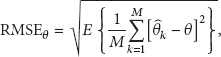
Unless otherwise specified, the performance of the investigated solutions has been assessed by measuring the root-mean-square error (RMSE) of the estimates at the steady state:

$$\begin{array}{cc}& \text{RMS}{\text{E}}_z=\sqrt{E\left\{\frac{\mathrm{1}}{M}{\displaystyle \sum }_{k=\mathrm{1}}^M{\left[z_k^{\left(N_s\right)}-\eta \right]}^{\mathrm{2}}\right\}},\end{array}$$

(44)

where η is given by

$$\begin{array}{cc}& \eta =\frac{\mathrm{1}}{M}{\displaystyle \sum }_{k=\mathrm{1}}^M‍z_k^{\left(\mathrm{1}\right)}\end{array}$$

(45)

while $N_s$ denotes the iteration index for which the algorithm achieves its steady state. In the sequel, such a state is achieved at the iteration index from which the variations of the $\text{RMS}{\text{E}}_z$ are limited in the range $\pm \mathrm{\hspace{0.17em}\hspace{0.17em}}\mathrm{1}{\mathrm{0}}^{-\mathrm{2}}$ . Interestingly, we have found through numerical results that the proposed algorithm is virtually unbiased, so the RMSE and the standard deviation of the estimation error are practically the same.

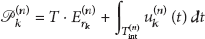
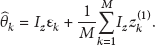
We now show how the $\text{RMS}{\text{E}}_z$ defined above can be used to compute the RMSE of the unknown parameter θ:

$$\begin{array}{cc}& \text{RMS}{\text{E}}_{\theta }=\sqrt{E\left\{\frac{\mathrm{1}}{M}{\displaystyle \sum }_{k=\mathrm{1}}^M{\left[{\widehat{\theta }}_k-\theta \right]}^{\mathrm{2}}\right\}},\end{array}$$

(46)

where ${\widehat{\theta }}_k$ denotes the estimate of θ at the kth sensor during the steady state. Recalling (1) and (2), we have that ${\widehat{\theta }}_k$ is given by

$$\begin{array}{cc}& {\widehat{\theta }}_k=I_z{z}_k^{\left(N_s\right)}.\end{array}$$

(47)

We now let ${\epsilon }_k=z_k^{(N_s)}-\eta$ and use (45) to rewrite the right-hand side of (47) in the following equivalent form:

$$\begin{array}{cc}& {\widehat{\theta }}_k=I_z{\epsilon }_k+\frac{\mathrm{1}}{M}{\displaystyle \sum }_{k=\mathrm{1}}^M‍I_z{z}_k^{\left(\mathrm{1}\right)}.\end{array}$$

(48)

From (1) and (2), we have that $I_z{z}_k^{(\mathrm{1})}=\theta +a_k+{\varsigma }_k$ , where $a_k$ is a random variable depending on the quantization error, which is assumed to be uniformly distributed within the range $\pm \mathrm{\hspace{0.17em}\hspace{0.17em}}{I}_z/\mathrm{2}$ .

Collecting all the above facts together and assuming that ${\epsilon }_k$ , $a_k$ , and ${\varsigma }_k$ are statistically independent, using standard computations, it follows that $\text{RMS}{\text{E}}_{\theta }$ takes the form

$$\begin{array}{cc}& \text{RMS}{\text{E}}_{\theta }=\sqrt{\frac{{\sigma }_{\varsigma }^{\mathrm{2}}}{M^{\mathrm{2}}}+I_z^{\mathrm{2}}\times \left(\text{MS}{\text{E}}_z+\frac{\mathrm{1}}{\mathrm{12}\times M^{\mathrm{2}}}\right)},\end{array}$$

(49)

where ${\sigma }_{\varsigma }$ denotes the standard deviation of the noise term ${\varsigma }_k$ . The above result is useful to evaluate the relationship between the estimation accuracy provided by each sensor working individually (represented by ${\sigma }_{\varsigma }$ ) with that ensured by consensus (given by $\text{RMS}{\text{E}}_{\theta }$ ). Assume, for example, that θ is a temperature and $M=\mathrm{20}$ . If ${\sigma }_{\varsigma }={\mathrm{3}}^{\circ }$ , $\text{MS}{\text{E}}_z$ = 0.5 (see, e.g., Figure 8) and $I_z={\mathrm{1}}^{\circ }$ , from (49), it follows that $\text{RMS}{\text{E}}_{\theta }=\mathrm{0.7}{\mathrm{2}}^{\circ }$ . This means that consensus may ensure estimation accuracy four times better than that of a single sensor.

5.2. Performance Evaluation

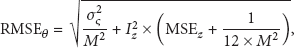
We begin by assessing the impact of the system parameters Δ and ${\mu }_{\mathrm{0}}$ on the performance of RC-BIE. Figure 6 illustrates the $\text{RMS}{\text{E}}_z$ of RC-BIE as a function of Δ for different values of ${\mu }_{\mathrm{0}}$ when the SNR is fixed to 25 dB, $M=\mathrm{20}$ , and $N_b=\mathrm{8}$ . We see that the best performance is obtained with ${\mu }_{\mathrm{0}}$ equal to 4 and that the $\text{RMS}{\text{E}}_z$ keeps practically constant for values of Δ larger than 25 ns, while an increase is observed for $\Delta <\mathrm{25}$  ns. Such a behavior suggests to choose a value of Δ greater than or equal to 25 ns. From (11), it is seen that Δ cannot be chosen arbitrarily large as it would increase the symbol duration and consequently the required converge time. To satisfy these two conflicting requirements, in all the subsequent simulations, we adopt $\Delta =\mathrm{25}$ , which corresponds to a symbol duration T of $\mathrm{0.77}\mathrm{\hspace{0.17em}\hspace{0.17em}}\mu$ s.

Figure 6

$\text{RMS}{\text{E}}_z$ of RC-BIE at the steady state as a function of ${\mu }_{\mathrm{0}}$ for different values of ${\mu }_{\mathrm{0}}$ with SNR = 25 dB, $N_b=\mathrm{8}$ , and $M=\mathrm{20}$ .

A close inspection of the results of Figure 6 indicates that the best performance at the steady state is achieved for ${\mu }_{\mathrm{0}}=\mathrm{4}$ . However, this fact is not enough to fix ${\mu }_{\mathrm{0}}=\mathrm{4}$ since the step size must be chosen so as to achieve a reasonable tradeoff between steady state performance and convergence capabilities. For this reason, in Figure 7, we illustrate how the $\text{RMS}{\text{E}}_z$ evolves in time with the iteration index for different values of ${\mu }_{\mathrm{0}}$ when the system parameters are the same of Figure 6. For this purpose, the performance is assessed by evaluating the $\text{RMS}{\text{E}}_z$ at the nth iteration, which is mathematically given by

$$\begin{array}{cc}& \text{RMS}{\text{E}}_z\left(n\right)=\sqrt{E\left\{\frac{\mathrm{1}}{M}{\displaystyle \sum }_{k=\mathrm{1}}^M{\left[z_k^{\left(n\right)}-\eta \right]}^{\mathrm{2}}\right\}}.\end{array}$$

(50)

From the results of Figure 7, we observe that RC-BIE has a very short convergence time as it achieves the equilibrium in only 3 μs when ${\mu }_{\mathrm{0}}=\mathrm{3}$ while 4 μs are needed for ${\mu }_{\mathrm{0}}=\mathrm{4}$ . Then, we may reasonably set ${\mu }_{\mathrm{0}}=\mathrm{4}$ as indicated by the results of Figure 6.

Figure 7

$\text{RMS}{\text{E}}_z(n)$ of RC-BIE versus $nT$ for different values of ${\mu }_{\mathrm{0}}$ with SNR = 25 dB, $N_b=\mathrm{8}$ , and $M=\mathrm{20}$ .

Figure 8

$\text{RMS}{\text{E}}_z$ of RC-BIE at the steady state as a function of SNR for different values of $N_b$ with Δ = 25 ns, ${\mu }_{\mathrm{0}}=\mathrm{4}$ , and $M=\mathrm{20}$ .

Figure 8 shows the $\text{RMS}{\text{E}}_z$ of RC-BIE as a function of SNR for different values of $N_b$ with Δ = 25 ns, ${\mu }_{\mathrm{0}}=\mathrm{4}$ , and M = 20. The curve labelled “No quantization” corresponds to the performance of RC-BIE when no quantization is employed at the receiver and serves a benchmark. As seen, reducing $N_b$ up to $\mathrm{6}$ does not affect appreciably the performance of RC-BIE for SNR values of practical interest. Since a small number of bits results into a quantizer of reduced complexity and lower energy consumption, we choose $N_b$ equal to 6 in all subsequent simulations.

Figure 9 depicts the $\text{RMS}{\text{E}}_z$ versus SNR when the number of active sensors is $M=$ 10, 20, and $\mathrm{30}$ . As expected, the $\text{RMS}{\text{E}}_z$ reduces as the SNR increases. Interestingly, we observe that in the low SNR regime increasing M improves the system performance while only marginal differences are observed for all the other SNR values of practical interest.

Figure 9

$\text{RMS}{\text{E}}_z$ of RC-BIE versus SNR in dB for different values of M with Δ = 25 ns, ${\mu }_{\mathrm{0}}=\mathrm{4}$ , and $N_b=\mathrm{6}$ .

We now return to the need of using a properly designed threshold to remove the noise contribution at the output of the square device. For this purpose, in Figure 10 we plot the $\text{RMS}{\text{E}}_z$ versus SNR for different values of λ. For comparisons, we report also the performance of a system in which the threshold is set to zero. From the results of Figure 10 it follows that our arguments in Section 4 were correct. In fact, a gain greater than 15 dB is achieved in all investigated scenarios in which the threshold is employed. As anticipated, the best results are obtained for λ such that $P_{\text{th}}(\lambda )=\mathrm{1}{\mathrm{0}}^{-\mathrm{5}}$ .

Figure 10

$\text{RMS}{\text{E}}_z$ of RC-BIE versus SNR in dB for different values of $P_{\text{th}}(\lambda )$ with Δ = 25 ns, ${\mu }_{\mathrm{0}}=\mathrm{4}$ , $N_b=\mathrm{6}$ , and $M=\mathrm{20}$ .

In Figure 11, we compare RC-BIE with BIE. Comparisons with BIE are made under a common simulation setup, which includes the same $\Delta =\mathrm{25}$  ns and ${\mu }_{\mathrm{0}}=\mathrm{4}$ as well as the same threshold λ. From the results of Figure 11, we see that RC-BIE has virtually the same $\text{RMS}{\text{E}}_z$ of BIE for all the investigated SNRs. This result is achieved with reduced complexity since the proposed solution operates with a much lower sampling frequency.

Figure 11

$\text{RMS}{\text{E}}_z$ of RC-BIE and BIE versus SNR in dB with Δ = 25 ns, ${\mu }_{\mathrm{0}}=\mathrm{4}$ , and $M=\mathrm{20}$ .

All the above results are obtained considering the CM1 scenario. We now assess how the propagation channel influences the system performance. For this purpose, Figure 12 illustrates the $\text{RMS}{\text{E}}_z$ versus SNR for the following channel propagation models: CM1, CM2, CM3, and CM4. The latter are four of the most representative channel models defined for the IEEE 802.15.4a standard (see [22] for more details). In particular, CM1 and CM2 applies to a line-of-sight (LOS) and a non-line-of-sight (NLOS) propagation in residential environments, respectively, while CM3 and CM4 reflect a LOS and a NLOS scenario in office environments. In particular, the building structures of residential environments are characterized by small units, with indoor walls of reasonable thickness and cover a range from 7 to 20 m. For office environments, some of the rooms are comparable in size to residential, but other rooms (especially cubicle areas, laboratories, etc.) are considerably larger. Areas with many small offices are typically linked by long corridors. Each of the offices typically contains furniture, bookshelves on the walls, and so forth, which adds to the attenuation given by the (typically thin) office partitioning. Office environments cover a range from 3 to 28 m. We observe that the best performance is achieved for CM1. However, changing the propagation channel incurs in a loss of less than 4 dB.

Figure 12

$\text{RMS}{\text{E}}_z$ of RC-BIE versus SNR in dB for different channel models with Δ = 25 ns, ${\mu }_{\mathrm{0}}=\mathrm{4}$ , $N_b=\mathrm{6}$ , and $M=\mathrm{20}$ .

6. Conclusions and Discussions

We have presented and investigated the behaviours of a physical layer scheme for achieving consensus in UWB sensor networks. The practical implementation issues of the proposed solution have been investigated and its performance has been deeply analyzed. Particular attention has been devoted to the study of the impact of the number of bits used by the quantizer on the system performance and to a proper design of the system parameters in order to achieve fast convergence time with high estimation accuracy. We have found that with a 6-bit resolution the loss, compared to an ideal receiver with no quantization, is not appreciably and that a steady state with negligible estimation errors can be achieved in less than 4  $\mu s$ . The performance has been evaluated under a practical simulation setup inspired to the IEEE 802.15.4a standards. On the basis of such an analysis, it turns out that the proposed scheme provides the same performance of an existing alternative based on an all-digital implementation. However, this result is obtained with a reduced complexity and low-energy consumption as it allows the receiver to operate at a much lower sampling frequency on the order of MHz instead of GHz. This makes it particularly suited for practical applications. To the best of our knowledge, this is the first time that an analysis on designing appropriate physical layer schemes to achieve consensus in practical applications is carried out. Indeed, most of the existing works in this field are largely focused essentially on the mathematical characterization of the conditions for achieving consensus. We hope that this work may act as an incentive to the research community for further investigating such problems. In particular, a hardware implementation for testing the performance of the proposed solution under real world conditions would be a very interesting topic for future research.