Sage Journals: Discover world-class research

Abstract

Wireless sensor networks (WSNs) can be used to monitor long linear structures such as pipelines, rivers, railroads, international borders, and high power transmission cables. In this case a special type of WSN called linear wireless sensor network (LSN) is used. One of the main challenges of using LSN is the reliability of the connections among the nodes. Faults in a few contiguous nodes may cause the creation of holes which will result in dividing the network into multiple disconnected segments. As a result, sensor nodes that are located between holes may not be able to deliver their sensed information which negatively affects the network's sensing coverage. Sensing robots can be used to overcome these faults and enhance the coverage. Sensing robots provide additional sensing coverage and restore the connectivity among disconnected segments. This paper develops a cost-effective design for robot-assisted fault-tolerant LSN. In this design the numbers of fixed sensor nodes and mobile sensing robots are determined such that the required reliability and sensing coverage levels are maintained while the total cost is minimized. The paper covers both uniformly and randomly deployed sensors LSNs.

1. Introduction

One of the important applications of LSN [1] is monitoring pipeline infrastructures such as gas, water, and oil pipelines [2, 3]. Such infrastructures could extend for thousands of meters in varying environments many of which are remote and usually unforgiving locations such as underwater [4]. Using LSN to monitor and in some cases control some aspects of these infrastructures has become important. Having a fault-tolerant LSN that would monitor and relay condition changes and environmental properties around the infrastructure allows the operators and management to make accurate decisions regarding maintenance, adjustments, replacements, and failure recovery activities.

Other applications of LSN are railroad/subway monitoring, AC power line monitoring, river monitoring, and border monitoring [1]. LSNs used for monitoring these structures consist of a number of sensor nodes. Each sensor node is equipped with sensing elements, a battery, a wireless communication device, a low-capability processor, a small memory, and a small storage. The sensors are lined through the structure to provide three main functions: sensing, information relay, and information filtering. The sensing function is to observe for any interesting changes in or around the monitored structure. The information relay helps forward observed data to the main station using multihop communication. The filtering function filters out and aggregates multiple pieces of sensed data into smaller messages. This will optimize communication, processing, and routing as well as the power needs thus extending the life of the network.

There are several reasons why new frameworks, protocols, and architectures are needed for different categories of LSNs as detailed in [1]. Such reasons include $(1)$ increased routing efficiency, $(2)$ increased network robustness and reliability, $(3)$ improved location management algorithms, and $(4)$ increased network security. As a result, different aspects of LSN have been investigated recently by some researchers. We developed a number of efficient routing protocols [2] and a distributed topology discovery algorithm [5] for LSN. Zimmerling et al. studied energy-efficient and localized power-aware routing in LSN [6, 7]. Noori and Ardakani proposed an analysis to characterize the traffic load distribution over a randomly deployed LSN [8]. Liu et al. provided an algorithm for an energy-balanced data gathering for LSN [9]. Li provided energy-efficient node replacement schemes in LSN to balance network load and extend network lifetime [10]. Finally, Martin and Paterson developed a lightweight key redistribution mechanism for LSN [11].

One of the main challenges facing LSN is losing connectivity in the network [12]. This is due to faults in neighboring and consecutive nodes. Nodes can fail due to battery exhaustion, hardware failures, and natural or intentional damages. These consecutive faulty nodes form holes which may cause the LSN to be divided into multiple disconnected segments. Some of these segments will become isolated; thus, they cannot transfer their sensed data to the main station. As a result the isolated segments will not provide any sensing coverage. Connectivity and coverage are generally considered very important issues in wireless sensor networks [13–16] and this issue is more challenging in LSNs due to its unique characteristic of limited availability of connection paths that can be used to overcome faults.

In this paper, we investigate the use of sensing robots (SRs) to enhance the reliability of LSNs. We develop and validate an analytical model to find the number of SRs needed to maintain highly reliable and fault-tolerant LSNs. In addition, this paper develops a methodology for cost-effective design. In this design the numbers of fixed sensor nodes and mobile sensing robots are determined such that the required reliability and sensing coverage levels are maintained while the total cost is minimized.

Our model is suitable for both uniformly deployed LSNs and randomly deployed LSNs. In uniform LSNs, the distances between any two neighboring nodes are equal, while in random LSNs, these distances are not. A uniform deployment may occur on pipeline infrastructures or power lines where sensors are distributed at equal distance from each other over the pipes or power towers. An example of random deployment occurs when sensors are dropped on site using an airplane or a moving vehicle [17] along a path to monitor a river bank [18] or a border [19]. We previously investigated different types of LSN applications and deployments in [1].

In the rest of this paper we cover the related work in Section 2. Section 3 provides background information about LSNs. The reliability and coverage issues of LSNs are covered in Section 4. In Section 5, we discuss using SRs and in Section 6 we develop a model to estimate the number of SRs needed for high reliability in uniform LSNs. A cost-effective design that combines both fixed and sensing robots in uniform LSNs is discussed in Section 7, while Section 8 provides examples and experiments. We extend our framework for randomly deployed LSNs in Section 9. In Section 10 we conclude the paper.

2. Related Work

There is some effort to utilize robots for enhancing deployments, operations, maintenance, and the life span of WSNs. Mobile robots were investigated for WSN deployments in normal situations [20] and in disaster situations [21]. Fletcher et al. [22] and Houaidia et al. [23] developed some robot-assisted relocation strategies of sensors for coverage enhancements for randomly deployed WSNs. Tong et al. [24] developed a strategy for reclaiming nodes with low or no power supply, replacing them with fully charged ones and bringing the reclaimed nodes back to an energy station for recharging. Mei et al. [25] developed and analyzed some algorithms to determine which best robot to replace a faulty node in large-scale static sensor networks. Some research effort was also dedicated for developing mechanisms for WSN localizations using mobile robots [26, 27]. These studies were done mainly for two-dimensional WSNs that are deployed at random.

Unlike in two-dimensional WSN in which sinks can be reached through multiple existing paths which can be utilized to enhance the reliability, very few alternate paths are usually available in LSNs [28]. Few nodes faults can significantly drop the network connectivity and coverage. We proposed to use mobile sensors to enhance the coverage in LSNs [29]. In this paper, we develop a framework for a cost-effective design for robot-assisted fault-tolerant LSN. This framework shows that using mobile sensor robots can not only enhance the coverage of LSNs but also it can reduce the cost on some configuration cases.

3. Linear Wireless Sensor Networks (LSNs)

Wireless sensor nodes can be installed on a linear structure to observe the status of the structure and its surrounding environment. These nodes can be deployed uniformly or randomly to form an LSN. In both types of LSNs, the nodes are distributed to cover the monitored structure. Sensing nodes usually have limited transmission compatibilities where each node can communicate with only a few neighboring nodes [3]. Nodes collaborate among themselves in both sensing and communication functions. Multihop communication is used to transfer the sensed and control data across the linear structure and to/from the main control station. Wireless networks can solve some of the reliability problems of current wired networks technologies that are used to monitor linear structures [2]. For example, WSNs can still function even when some nodes are disabled. Faults in sensor nodes can be easily tolerated using other available nodes to cover the faulty ones. Using dense LSNs with a high number of nodes and/or using wide wireless transmission ranges, the network can maintain connectivity and the sensed and control data can be transmitted through the network to its destination even with the existence of some node faults. For example, in the uniform LSN in Figure 1, each node can communicate with two nodes to the left and two nodes to the right. If for example nodes 3 and 5 are damaged, node 4 can still send its sensed data through node 2 or 6. The maximum number of neighboring nodes that each node can communicate with each side can be defined as a maximum jump factor (MJF).

Figure 1

Reliability in a dense uniform LSN.

For example, MJF in Figure 1 is 2; thus, node 4 can communicate with a maximum of two nodes on each side.

Each senor node on a linear structure is usually equipped with a transceiver, a processor, a battery, memory, and small storage in addition to one or more sensing elements. Power consumption is critical to the life span of LSNs. Linear structures need to be monitored throughout their life span which could extend to tens of years. Therefore, the associated LSNs should also be long lived. Unlike wired networks where the power is not at all a constraint as the wires deliver power to the different sensor nodes, LSN designers have to consider power as one of the main constraints in the wireless system. Power in a sensing node is consumed by every element on it. A transceiver consumes power waiting for a signal and when transmitting or receiving data. Sensing elements also consume power and the processor as well. Careful scheduling of these resources is needed to optimize power consumption. Although increasing transmission range offers better communication reliability, the nodes will consume more energy. A dynamic configuration for the wireless transmission range can provide better power management. An example of this configuration of a uniform LSN is in Figure 2. Here, nodes 3 and 5 have failed. Therefore, the wireless range for node 4 is increased to reach nodes 2 and 6, while other nodes use a smaller transmission range to reduce the power consumption. The sensed data is transferred through the line to the main station in either direction or both if both directions are connected to the main station. Connecting both directions to the main station will double the communication reliability [3, 4].

Figure 2

Automatic wireless range configuration.

4. Faults and Coverage in LSN

Sensor nodes are usually initially distributed to cover the whole linear structure in terms of both sensing and communication coverage. A node senses interesting events and this observation is reported to the main station using multihop communication. Sensors in LSN nodes can have different sensing range capabilities. In a uniform LSN where nodes are distributed at uniform distances, let us define the distance between two neighboring nodes i and $i + 1$ as one distance unit. Then an LSN with healthy nodes can provide 100% sensing coverage for the monitored linear structures if the node sensing range (NSR) is one distance unit.

This coverage is reduced if there are some faulty nodes. However, if NSR is larger than d (one distance unit), then some node faults can be easily tolerated without reducing the percentage of the sensing coverage. For example, if NSR is 2 distance units. This means that the area between two neighboring nodes i and $i + 1$ is monitored twice by both nodes. In this case, this area will be still under monitoring even if node i or node $i + 1$ is faulty.

LSN is usually designed to provide a full sensing coverage. However, after some time, there will be some faults among the nodes. Let us consider that we have a one-segment network with homogeneous nodes. Let us also assume that there is a uniform distance between each two nodes. In addition, nodes have a specific MJF. Let us define a term Hole (H) as the number of contiguous faulty nodes in the LSN. Each hole can be of size of one or more nodes. 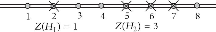For example, in Figure 3, we have two holes: $H_{1}$ and $H_{2}$ . The first one is with size 1 where only node 2 is faulty while the second hole, $H_{2}$ , is of size 3 where nodes 5, 6, and 7 are faulty. We use $Z (H_{1}) = 1$ and $Z (H_{2}) = 3$ where Z is the size function of a hole. In addition, we can use $R (H_{i}) = [F_{i} : L_{i}]$ to specify the ID of first faulty node, $F_{i}$ , and the ID of last faulty node, $L_{i}$ , in $H_{i}$ . Thus, we have $Z (H_{i}) = L_{i} - F_{i} + 1$ .

Figure 3

Two holes in the LSN.

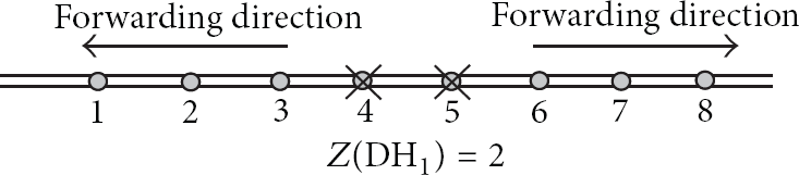
A special type of hole is a disconnecting hole (DH), which disconnects the network into two segments that cannot directly communicate with each other using an extended wireless range. In other words, the size of a DH is larger than or equal to the MJF used for the nodes in the LSN, $Z (DH) \geq MJF$ . For example, if the MJF of the LSN in Figure 3 is 2, then $H_{2}$ is DH while $H_{1}$ is not. This is because $Z (H_{2}) = 3$ which is larger than the MJF, while $Z (H_{1}) = 1$ which is less than the MJF.

There are different types of faults in a one-segment LSN with homogenous nodes distributed uniformly over the linear structure. Assume that both ends of the LSN are connected to the main station. The faults have different impacts on the communication and sensing coverage. For example, if there are multiple holes that are all not disconnecting holes, then the LSN will function normally. Although there will be some holes with sizes smaller than MJF, any sensed information can be transferred to the main station through the left or right side of the network. Any hole can be jumped over by extending the wireless range of the node that forwards the sensed data to the MJF to reach the next functioning node. The sensing coverage in each hole may or may not be affected. This depends on the size of the hole and NSR. Let $U (H_{i})$ be the size of the uncovered sensing area in $H_{i}$ :

\begin{matrix} U (H_{i}) = {\begin{cases} 0 & Z (H_{i}) < NSR \\ Z (H_{i}) - (NSR - 1) & otherwise . \end{cases} \end{matrix}

(1)

For example, if $Z (H_{i})$ is 3 and NSR is 4, then $U (H_{i})$ is 0. In another, if $Z (H_{i})$ is 6 and NSR is 3, then $U (H_{i})$ is 4. If there are n nodes and k holes in an LSN, then the sensing coverage percentage, C, is

\begin{matrix} C = \frac{n - \sum_{i = 1}^{k} U (H_{i})}{n} . \end{matrix}

(2)

In another fault case, there are multiple holes; only one of them is a disconnecting hole. In this case the LSN will continue to function. This one DH will divide the LSN into two segments: one on the left side of the DH and the other is on the right side. As the size of the DH is larger than or equal to MJF then this DH will disable information exchange between both segments as shown in Figure 4. In this case, all healthy nodes on the left side of the DH will use a right-to-left forwarding direction, while all healthy nodes on the right side will use a left-to-right forwarding direction to communicate with the main station.

Figure 4

LSN with $MJF = 2$ . LSN is divided into two segments by a DH. Each one will communicate in a different direction.

The sensing coverage of LSN can be calculated using (1) and (2). In the example shown in Figure 5, the size of DH is 3, while NSR is 4; then the healthy nodes 6 and 10 cover the whole area of DH. In another example (see Figure 6) the size of DH is 5, while NSR is 4. In this case, there are 2 distance units that are not covered by both healthy nodes 6 and 12.

Figure 5

LSN with $MJF = 2$ . $Z (DH) = 3$ and $NSR = 4$ . The whole DH is covered.

Figure 6

LSN with $MJF = 2$ , $Z (DH) = 5$ , and $NSR = 4$ . The whole DH is not covered.

In another fault case, there are multiple holes; only two of them are disconnecting holes. In this case, the LSN will be divided into three segments. Let the DHs be DH₁ and DH₂. The first segment is before DH₁, the second segment is between DH₁ and DH₂, and the third segment is after DH₂ as shown in Figure 7. In this figure, DH₁ is from node 5 to node 6 while DH₂ is from node 11 to node 13. The first segment covers nodes 1 through 4, the second covers nodes 7 through 10, and the third covers nodes 14 through 17. All nodes in the first segment can communicate with the main station in the right-to-left direction, while all nodes in the third segment can communicate with the main station in the left-to-right direction. However, healthy nodes in the second segment cannot communicate with the main station at all.

Figure 7

LSN with $MJF = 2$ . There are two DHs: DH₁ and DH₂. The segment between DH₁ and DH₂ is not connected.

In another case, there are multiple holes with more than two disconnecting holes. Here we assume that there are k DHs: DH₁ through ${DH}_{k}$ . Thus, the LSN will be divided into $k + 1$ segments. With the existence of k DHs, all nodes starting from the first node in DH₁ through the last in ${DH}_{k}$ will not be able to communicate with the main station. As a result, the areas from DH₁ to ${DH}_{k}$ will be uncovered. The effect of this type of fault on the network coverage is similar to having a large disconnected hole, ${DH}_{1, k}$ that extends from the first node in DH₁ to the last node in ${DH}_{k}$ in the network. Equations (1) and (2) are to find the uncovered areas as well as the coverage percentage due to this large DH.

5. Using Sensing Robots

Mobile sensing robots (SR) can be used to enhance the communication and sensing coverage in LSNs. SRs are equipped with all the components a sensing node has including sensors, processor, memory, storage, and wireless transmitter/receiver in addition to some specialized robot devices. Each SR can move linearly over the LSN to cover a DH and provide sensing and communication coverage as shown in Figure 8. When placed at a DH, the SR provides connectivity in the disconnected segments in addition to sensing coverage. If MJF is 2, then one SR can cover a DH with size up to 3 nodes. Generally each SR can cover a DH with a maximum size of ( $2 * MJF - 1$ ). If the size of a DH is larger than ( $2 * MJF - 1$ ) then two or more SRs are needed as shown in the equation for the number of SRs:

\begin{matrix} m_{Z (DH)} = ⌊ \frac{Z (DH)}{MJF} ⌋ . \end{matrix}

(3)

Figure 8

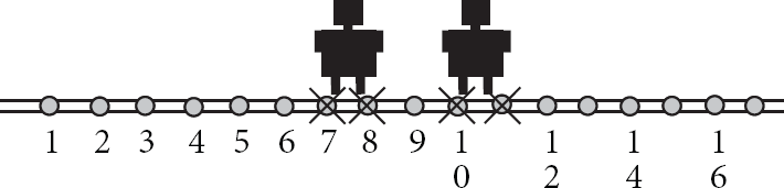
LSN with $MJF = 2$ and two DHs.

Multiple SRs can be distributed across the linear structure to provide recovery from any DHs. They can also be reallocated to different locations as new DHs occur to maintain best possible sensing coverage. To understand the importance of SR reallocations assume that the current status of the LSN is as shown in Figure 8. MJF is 2 while only two SRs are available and they are already used to cover two existing DHs as shown in Figure 8. Using these two SRs, the whole LSN is covered. Now assume that after some time, two more DHs occurred in the LSN as shown in Figure 9, thus making four DHs. The new DHs will reduce the coverage significantly as all the area (14 nodes) from node 2 to 15 will be uncovered. The assigned SRs are reallocated to cover DH₁ and DH₄ instead of DH₂ and DH₃. The result is shown in Figure 9, where the reallocation resulted in leaving only 5 nodes from 7 to 11 without coverage compared to 14 nodes earlier.

Figure 9

Reallocation of SRs for better coverage.

Let A be the number of available SRs and let R be the number of needed SRs to cover all DHs. The best strategy to use for SR reallocation in case we need more SRs than available (i.e., $R > A$ ) is to complete the coverage such that the smallest disconnected segment is left out. That is, we need to find the shortest segment that needs ( $R - A$ ) SRs without placing any SRs while placing the available SRs in the remaining DHs. The main reason of not covering the shortest segment is to minimize the uncovered area and to maximize the coverage area.

6. Estimating the Number of SRs

For good network coverage, it is important to know the number of SRs needed to cover possible DHs in the LSN. In this section, we develop an analytical model that provides a way to estimate the number of SRs needed to maintain high LSN coverage. Given an LSN with n uniformly distributed nodes and a specific MJF, each node has a chance to independently fail with probability f within a certain period of time T. T can be the time to a periodic full maintenance or the time that the LSN is needed to live. To know the number of needed SRs (R), we first need to know the expected number of holes that may occur and their sizes within time T. Knowing the number and sizes of the holes is essential to estimate the number of SRs to cover these holes. To know about the expected holes, let us first find the probability equation that a healthy node in the LSN has a hole directly in front of it with exactly size i. We name this equation $W_{i} (f)$ :

\begin{matrix} W_{i} (f) = {(1 - f)}^{2} \times f^{i} . \end{matrix}

(4)

Here, as f increases, the chance to have a healthy node with a hole with size i in front of it also increases. As there are n nodes in the LSN and all nodes other than the last i nodes that cannot have a hole of size i in front of them have the same chance to have a hole in front of it, then the number of holes of size i in the LSN is

\begin{matrix} N H_{i} (n, f) = W_{i} (f) \times (n - i) . \end{matrix}

(5)

By replacing

W_{i}

(f) with (4), we have

\begin{matrix} N H_{i} (n, f) = {(1 - f)}^{2} \times f^{i} \times (n - i) . \end{matrix}

(6)

Here, as the LSN size increases the chance to have more holes in the LSN also increases. Now, let $R_{i} (n, f, M J F)$ be the number of needed SRs to cover all expected holes with size i. We have

\begin{matrix} R_{i} (n, f, MJF) = N H_{i} (n, f) \times m_{i}, \end{matrix}

(7)

where

m_{i}

is the number of SRs needed to cover a hole with size i. We can replace

m_{i}

with (3):

\begin{matrix} R_{i} (n, f, MJF) = N H_{i} (n, f) \times ⌊ \frac{i}{MJF} ⌋ . \end{matrix}

(8)

For any realistic value for f, it is usually a very low probability to have holes with sizes larger than a certain number in an LSN. Therefore, we can consider that we have a variable v that represents the maximum size of possible holes. Let $R (n, f, MJF)$ be the expected number of total SRs needed to cover all disconnected holes. We have

\begin{matrix} R (n, f, MJF) = ⌈ \sum_{i = MJF}^{v} R_{i} (n, f, MJF) ⌉ . \end{matrix}

(9)

To validate the above equations, a number of simulation experiments were conducted covering different LSN configurations as listed in Table 1. These LSN configurations have different number of nodes (n), node fault rate (f), maximum jump factor (MJF), and node sensing range (NSR). The table also lists the expected numbers of needed SRs for all LSN configurations. These numbers are calculated using (9).

Table 1

Different LSN configurations.

Net.	n	f	$MJF$	NSR	R
LSN1	2000	5%	2	2	5
LSN2	500	12%	2	2	7
LSN3	1500	22%	3	3	13
LSN4	500	20%	2	2	17
LSN5	1000	15%	2	2	20

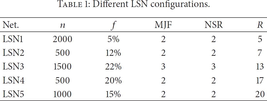
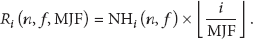
A set of simulation experiments were conducted for the LSNs with the configurations listed in Table 1. The experiments covered a setup without the reallocation strategy (WRS) with R replaced sensor nodes, where R is calculated from (9) and listed in Table 1. In addition, the experiments were conducted to find the impact of using different numbers of SRs on the coverage using, $R - 4$ , $R - 3$ , $R - 2$ , $R - 1$ , R, and $R + 1$ SRs. The main purpose of these experiments is to find the impact of using different number of SRs on the coverage and to validate whether using calculated R SRs will be enough to maintain high coverage. In other words, this will investigate whether using less than R SRs will decrease the expected coverage while using more than R SRs will not increase the expected coverage significantly.

For each simulation experiment, 10,000 different faulty LSN cases were generated randomly to cover different types of faults for each situation. The average of these 10,000 cases was calculated as an expected result for each experiment. The results are shown in Figure 10. As we can see, using R SRs ensures high coverage for all selected network configurations. The expected coverage is between 97% and 98% in all cases. This is generally a good coverage range. On the other hand, the expected coverage results of using less than R SRs significantly dropped as we use less SRs. At the same time, using more SRs, more than R, will slightly enhance the expected coverage of the LSN. These results validate the developed equations.

Figure 10

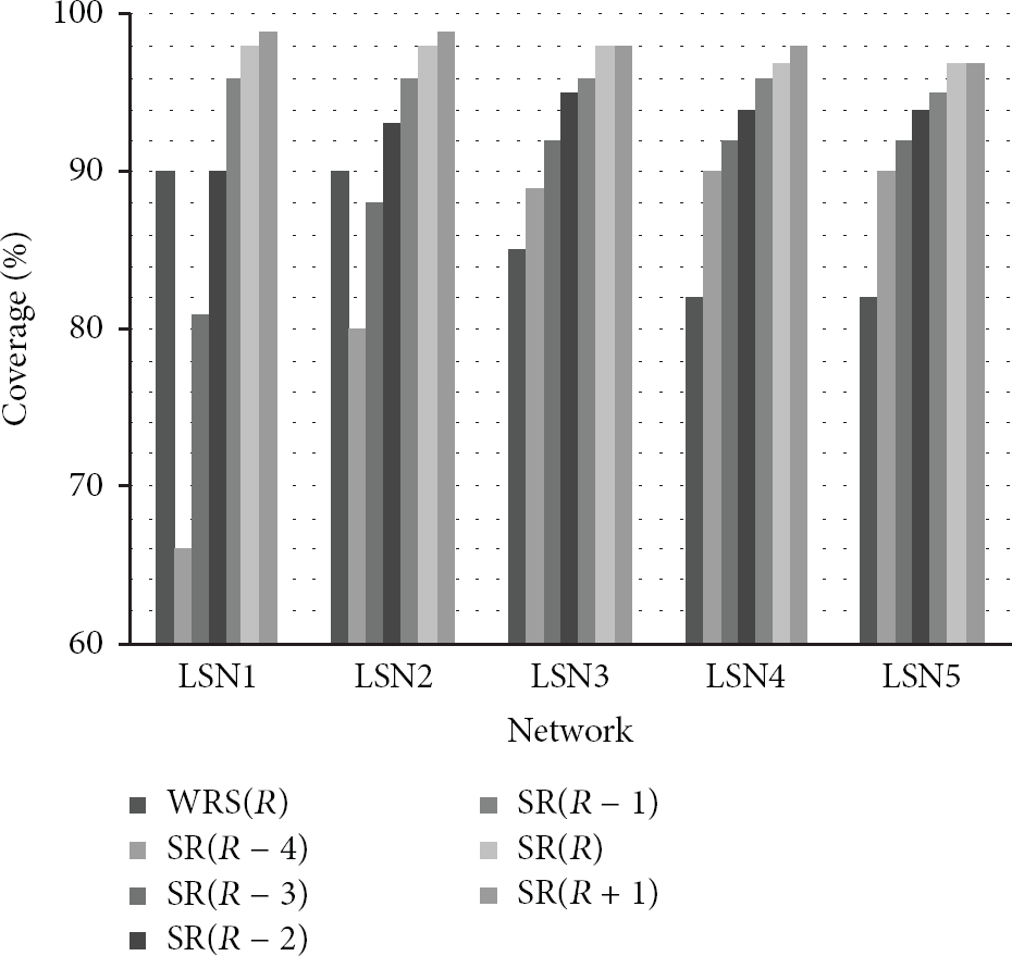
Expected coverage under different cases.

The coverage percentage range of 97% to 98% when using R SRs is obtained due to the existence of holes that are not disconnecting holes in the network. These holes will only slightly reduce the coverage. However, the SRs will cover most of the disconnecting holes; thus, the coverage will not drop significantly.

7. Cost Effective Design

In the previous section we developed an analytical model to find the numbers of SRs needed to maintain high coverage for LSNs. In the section, we develop a technique to design cost effective LSNs that combine both fixed sensor nodes and SRs. Let us assume that a linear area needs to be monitored with a LSN. For this LSN, a high coverage needs to be maintained for a time period T. T can be the time to a periodic full maintenance or the time that the LSN is needed to live. The LSN has a combination of fixed sensors and SRs. Let us assume that each fixed node has a chance to independently fail with probability f within the period T and SRs are designed to be highly reliable and of high quality. Let us assume that the cost of each fixed sensor node is one unit and the cost of each SR is Q units. In other words, the cost of each SR is Q times more than the cost of a fixed sensor. This is mainly due to the mobility feature of the SRs and the additional costs of needed functional units. The objective here is to find how many fixed sensor nodes and SRs are needed to maintain high coverage during the period T such that the total cost of the LSN is minimized.

To find the needed numbers of fixed sensor nodes (n) and SRs (R), we need to first find the minimum number of fixed nodes needed to have full connectivity in the LSN ( $n_{\min}$ ). Full connectivity is obtained when we have MJF as 1. Let the length of the area to be monitored be L. Assume that the maximum wireless range for each node is W. This means that each fixed sensor can communicate with one node on either side if each fixed node is placed at the maximum distance of W from each other. This means that the minimum number of fixed sensor nodes needed to maintain a full connectivity is

\begin{matrix} n_{\min} = ⌈ \frac{L}{W} ⌉ . \end{matrix}

(10)

For full coverage we can use LSNs with $1 \cdot n_{\min}$ , $2 \cdot n_{\min}$ , or $i \cdot n_{\min}$ nodes where i is the MJF. Each of these options needs a different number of fixed nodes and SRs to maintain high coverage within the period T. Let the total cost of fixed sensors be ${COST}_{S}$ and let the total cost of sensing robots be ${COST}_{R}$ :

\begin{matrix} COS T_{S} = MJF \times n_{\min}, \\ COS T_{R} = R (MJF \times n_{\min}, f, MJF) \times Q . \end{matrix}

(11)

The number of SRs, R, needed for each option can be found using (9). The total cost (TC) of each LSN option can be found by

\begin{matrix} T C_{Q} (n_{\min}, f, MJF) = COS T_{S} + COS T_{R} . \end{matrix}

(12)

We can calculate the total cost of the different options from 1 to j for MJF where j is the minimum MJF value to have a full LSN coverage during the period T using only fixed sensor nodes without using any SRs. These different deigns may have $n_{\min}$ , $2 \cdot n_{\min}$ , $3 \cdot n_{\min}, \dots$ , and $j \cdot n_{\min}$ fixed sensor nodes with $1, 2, 3, \dots$ , and j MJF, respectively. These options need different numbers of SRs to maintain high coverage. These SR numbers can be calculated from (9). As we double the MJF value, the value of NSR will also double due to the increase of the density of the fixed sensor nodes. We can find the total cost of all these design options with different numbers of fixed nodes and mobile nodes from (12). The option with the minimum total cost is the most cost effective to be considered for the LSN.

8. Example and Experiments

As an example, assume that fixed sensor nodes will be used to form a LSN. Each node has f as 0.25 during a period T. We assume that f is high since T is a long period. Assume that $n_{\min}$ is 200. Table 2 shows the total cost of different possible options for the LSN designs for three different Q values: 10, 20, and 50. In the table the number of needed SRs (R) is calculated from (9), while the total costs (TC) are calculated from (12).

Table 2

Total costs of different LSN solution designs.

Sol.	$MJF$	$NSR$	$n = MJF * n_{\min}$	R (9)	${TC}_{10}$ (12)	${TC}_{20}$ (12)	${TC}_{50}$ (12)
1	1	1	200	50	700	1200	2700
2	2	2	400	20	600	800	1400
3	3	3	600	8	680	760	1000
4	4	4	800	3	830	860	950
5	5	5	1000	1	1010	1020	1050
6	6	6	1200	0	1200	1200	1200

As we can see the best option when the total cost of each SR is 10 times the cost of a fixed sensor node, then the best cost effective design is to use 400 fixed sensor nodes and 20 SRs. In this case, MJF will be 2. The best option is when the total cost of each SR is 20 times the cost of a fixed sensor node; then the best cost effective design is to use 600 fixed nodes and 8 SRs. The best option is when the total cost of each SR is 50 times the cost of a fixed sensor node; then the best cost effective design is to use 800 fixed nodes and 3 SRs. These best cost effective designs in all three different fixed nodes and SR cost factor will provide high levels of coverage and some cost saving comparing to use more fixed sensor nodes to maintain the high coverage. The cost saving is around 50%, 36.7%, and 20.8% for $Q = 10$ , $Q = 20$ , and $Q = 50$ , respectively. This shows that using sensing robots in a fixed sensor node network can provide some cost savings in some cases.

To validate the different LSN designs listed in Table 2, two sets of simulation experiments were conducted. The experiments simulate coverage, where each LSN is initially deployed to provide full coverage. However, after some time, some faults will occur in some nodes thus reducing the coverage in the LSN. Here the LSN needs maintenance to regain full coverage again. The simulations were developed using a Java program, where experimental situations were created with 10,000 LSNs that were generated randomly to have different types of faults for each situation. The results are the averages measured from all these faulty LSNs. The first set was to check if all possible designs will provide high coverage with the existence of faults. The results are shown in Figure 11, where all solutions maintain high coverage with the existence of faults. Therefore, any design can be used; however, these designs have different costs.

Figure 11

Expected Coverage of different LSN designs.

The second set was conducted to compare using the cost effective design with varying numbers of SRs. The main purpose of this experiment is to find the impact of using different numbers of SRs on the coverage and to validate whether using the calculated R SRs will be enough to maintain high coverage. In other words, will using less than R SRs decrease the expected coverage while using more than R SRs not increase the expected coverage significantly. The experiments were conducted for $Q = 10$ , $Q = 20$ , and $Q = 50$ . The results are shown in Figures 12, 13, and 14 for $Q = 10$ , $Q = 20$ , and $Q = 50$ , respectively. As we can see, using R SRs ensures high coverage for all selected network configurations. The expected coverage is between 96.5% and 99% in all cases. This is generally a good range. On the other hand, the expected coverage using less than R SRs significantly drops. At the same time, using more SRs than R will slightly enhance the expected coverage of the LSN. These results validate the developed model.

Figure 12

Expected coverage for $Q = 10$ with the cost-effective design 2: $n = 400$ , $MJF = 2$ , $NSR = 2$ , and $R = 20$ .

Figure 13

Expected coverage for $Q = 20$ with the cost-effective design 3: $n = 600$ , $MJF = 3$ , $NSR = 3$ , and $R = 8$ .

Figure 14

Expected coverage for $Q = 50$ with the cost-effective design 4: $n = 800$ , $MJF = 4$ , $NSR = 4$ , and $R = 3$ .

9. Randomly Deployed LSN

In the previous sections we mainly developed and validated the cost-effective design framework for robot-assisted fault-tolerant uniformly deployed LSNs. However, sensor nodes for LSN can be deployed in a random fashion in some practical scenarios. One example of such a deployment is when the sensor nodes are dropped from an aircraft, ground vehicle, or underwater vehicle along a given path [17]. One example of this deployment can be used to form an LSN that monitors the area surrounding a long pipeline in unattended area to provide some sort of fast monitoring to prevent some external intentional and nonintentional threats [4]. The deployed sensors can report, for example, about any movement, sound, or hazards around the area of the pipeline for fast safety actions including sending security and emergency vehicles to the area [3].

Another example is when an autonomous underwater vehicle drops underwater sensor nodes for sea-boarder monitoring [30]. In these examples, although the aim is to deploy sensor nodes uniformly to cover the complete linear structure, the nodes are most likely deployed randomly with varying distances between each two neighboring nodes. Actual landing locations of sensor nodes may deviate from their targeted locations because of environmental factors such as winds or waves or geographic factors such as slopes and valleys. In this type of deployment, some sensor nodes may be damaged. As a result the network connectivity and sensing coverage capabilities may be significantly impacted. In this section we customize the framework to include randomly deployed LSNs. Two possible solutions for this problem are either to deploy more redundant fixed sensor nodes or to use a combination of fixed sensor nodes and reliable mobile sensor robots as we propose in this paper. In the latter case, a cost-effective design is needed to determine the number of fixed sensor nodes and mobile sensor robots needed in the network.

Assume that there is a plan to deploy a node for each $D_{1}$ meters distance to form a fully connected LSN with a minimum number of nodes while there is a change for some errors in the deployment with the maximum of $\pm e$ meters where $| e | < D_{1}$ . This means that the maximum distance between any two neighboring nodes is $D_{1} + 2 e$ meters, while the minimum distance between any two neighboring nodes is $D_{1} - 2 e$ meters. These distances are formed when one of the two neighboring nodes is placed at a position with the error of $+ e$ from its targeted location while the other is placed at a position with the error of $- e$ from its targeted location. If the maximum wireless range for each node is W, then we need to have $D_{1} + 2 e \leq W$ for full connectivity. To minimize the number of used sensor nodes, we can have $D_{1} + 2 e = W$ .This equation can be used to calculate the planned distance, $D_{1}$ . We have $D_{1} = W - 2 e$ . This means if one node is deployed after each $D_{1}$ meters and there is no fault in any of the nodes, then the network will be fully connected. Here in this case, we can consider that MJF is 1. Let the length of the area to be monitored be L. This means that the minimum number of fixed sensor nodes needed to maintain full network connectivity is

\begin{matrix} n_{\min} = ⌈ \frac{L}{D_{1}} ⌉ . \end{matrix}

(13)

Now, to make MJF equal to 2, we need to have 3 nodes placed in the range of W meters. These 3 nodes can be deployed with some random errors of the range of 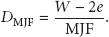$\pm e$ . We do not care about the location of the middle node as both side nodes can reach it regardless of the deployment error. However, the first node can be deployed with the error of $- e$ while the last one can be deployed with the error of $+ e$ . Thus, the maximum distance between the first and the last one will be $2 D_{2} + 2 e$ where $D_{2}$ is the planned deployment distance between each bode. This means that to maintain the MJF of 2 in the network, we need to have $2 D_{2} + 2 e \leq W$ . To minimize the number of deployed nodes in the network, we need to have $2 D_{2} + 2 e = W$ . This calculation maintains the connectivity of MJF of 2 in the network even if there are some random deployment errors. Similarly for $MJF > 2$ , we do not care about the deployment of the middle nodes but the location of the first and the last one in each W meter. Thus, $MJF \cdot D_{MJD} + 2 e \leq W$ and for minimizing the number of nodes on the network we need to have $MJF \cdot D_{MJD} + 2 e = W$ . Thus, for different values of MJF, the planned distance between any two neighboring nodes can be calculated as

\begin{matrix} D_{MJF} = \frac{W - 2 e}{MJF} . \end{matrix}

(14)

The number of needed nodes for different MJF configurations can be calculated as

\begin{matrix} n_{MJF} = ⌈ \frac{L}{D_{MJF}} ⌉ . \end{matrix}

(15)

As an example, let us consider that there is a need for a LSN to monitor an area of length 75,000 meters. The wireless communication range, W, of the nodes is 400 meters while f is 0.25. The error in the deployment is in the range of ±19 meters. The planned deployment distance and the number of needed sensors for different MJF configurations are shown in Table 3. The needed number of SRs, R, to maintain high reliability can be found from (9) while total cost can be found by

\begin{matrix} T C_{Q} = n_{MJF} + R \times Q . \end{matrix}

(16)

The cost of each fixed sensor node is one unit and the cost of each SR is Q units. In Table 3, Q is equal to 20 units.

Table 3

Different randomly deployed LSN configurations.

$MJF$	$D_{MJF}$ (14)	$n_{MJF}$ (15)	R (9)	${TC}_{20}$ (16)
1	362	208	52	1248
2	181	415	21	835
3	120	625	8	785
4	90	834	3	894
5	72	1042	1	1062
6	60	1250	0	1250

As we can see from Table 3, the most cost-effective configuration is when we use the MJF of 3. In this case, we need to use 625 fixed nodes that are placed each 120 meters and 8 SRs. This configuration only costs 785 units.

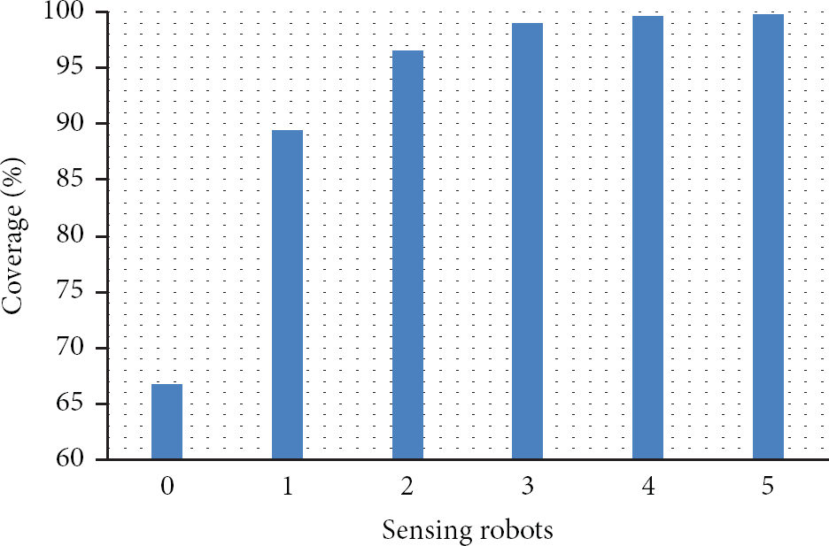
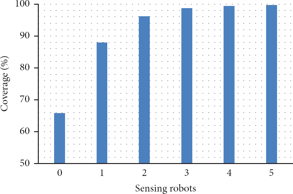
To validate the result, a simulation experiment was conducted to measure the sensing coverage of the most cost-effective configuration LSN with the MJF of 3. In this experiment, we measure the coverage with varying numbers of available SRs including less and more than the number needed. While the needed SRs are 8 based on Table 3, we experimented with numbers from 1 SR to 10 SRs. The simulation was developed using a Java program, where experimental situations were created with 10,000 LSNs that were generated randomly to have different types of faults and node deployment distances for each situation. The final results are the averages measured from all these LSNs. The sensor nodes in the experiments were distributed randomly using Gaussian distribution. This distribution represents a good model for generating random deployment WSN and used in many research papers in the field [17, 31–33].

The result is shown in Figure 15, where we see that using 8 SRs ensures high coverage. The expected coverage is around 97%, which is generally a good percentage. On the other hand, the expected coverage using less than 8 SRs significantly drops. At the same time, using more SRs than 8 will slightly enhance the expected coverage of the LSN. This result validates the developed model.

Figure 15

Expected coverage for randomly deployed LSN, with $MJF = 3$ , $D = 120$ , $n = 625$ , $e = \pm 19$ , and $W = 400$ .

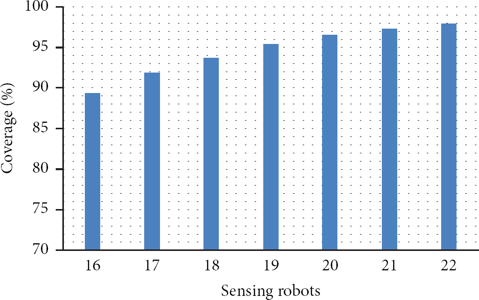
Two more sets of experiments were conducted to measure the impact of the number of SRs in the coverage on two LSN configurations with the MJF of 2 and with the MJF of 4. Both configurations provide good coverage if the right numbers of SRs are used, 21 and 3, respectively. However, both solutions cost more than the LSN with the MJF of 3. The results are shown in Figures 16 and 17. As the two figures show, using less than the calculated SRs can significantly drop the expected coverage, while using more than the calculated SRs will slightly enhance the coverage.

Figure 16

Expected coverage for randomly deployed LSN, with $MJF = 2$ , $D = 181$ , $n = 415$ , $e = \pm 19$ , and $W = 400$ .

Figure 17

Expected coverage for randomly deployed LSN, with $MJF = 4$ , $D = 90$ , $n = 834$ , $e = \pm 19$ , and $W = 400$ .

10. Conclusion

This paper discussed the use of sensing robots to create fault-tolerant LSNs by enhancing the communication and coverage reliability of these networks. A reallocation strategy of the sensing robots was developed to improve the coverage caused by node faults. An analytical model was developed to estimate the number of sensing robots needed to provide high coverage. In addition, a cost-effective design for fault-tolerant LSN with fixed sensors and sensing robots was developed for both uniformly and randomly deployed LSNs. The developed model provides an effective solution for enhancing the coverage in the presence of faults. This makes the proposed model suitable for critical applications for infrastructures located in difficult areas or harsh terrains that cannot be easily reached such as underwater pipelines that extend for hundreds of miles at depths that could exceed hundreds of meters. Incorporating the model at the LSN design stage will allow the LSN designers to have an accurate estimate of the number of nodes and SRs needed to maintain a high coverage during the lifespan of the LSN while minimizing the total cost.

Footnotes

Conflict of Interests

The authors declare that there is no conflict of interests regarding the publication of this paper.

Acknowledgment

This work is supported in part by UAEU Research Grant no. 3IT008.

References

Jawhar

Mohamed

Agrawal

D. P.

Linear wireless sensor networks: classification and applications

Journal of Network and Computer Applications 2011 34 5 1671 1682

2-s2.0-79960902911

10.1016/j.jnca.2011.05.006

Jawhar

Mohamed

M. M.

Aziz

A routing protocol and addressing scheme for oil, gas, and water pipeline monitoring using wireless sensor networks

Proceedings of the 5th IEEE/IFIP International Conference on Wireless and Optical Communications Networks (WOCN '08)

May 2008

Surabaya, Indonesia

1 5

2-s2.0-51049100194

10.1109/WOCN.2008.4542530

Mohamed

Jawhar

A fault tolerant wired/wireless sensor network architecture for monitoring pipeline infrastructures

Proceedings of the 2nd International Conference on Sensor Technologies and Applications (SENSORCOMM '08)

August 2008

Cap Esterel, France

179 184

2-s2.0-55949104674

10.1109/SENSORCOMM.2008.116

Mohamed

Jawhar

Al-Jaroodi

Zhang

Sensor network architectures for monitoring underwater pipelines

Sensors 2011 11 11 10738 10764

2-s2.0-82055165461

10.3390/s111110738

Jawhar

Mohamed

Zhang

A distributed topology discovery algorithm for Linear Sensor Networks

Proceedings of the 1st IEEE International Conference on Communications in China (ICCC '12)

August 2012

Beijing, China

775 780

10.1109/ICCChina.2012.6356988

Zimmerling

Dargie

Reason

J. M.

Energy-efficient routing in linear wireless sensor networks

Proceedings of the IEEE Internatonal Conference on Mobile Adhoc and Sensor Systems (MASS '07)

October 2007

Pisa, Italy

1 3

2-s2.0-50249120172

10.1109/MOBHOC.2007.4428618

Zimmerling

Dargie

Reason

J. M.

Localized power-aware routing in linear wireless sensor networks

Proceedings of the 2nd ACM International Conference on Context-Awareness for Self-Managing Systems (CASEMANS '08)

May 2008

Sydney, Australia

24 33

2-s2.0-57749114596

10.1145/1367943.1367946

Noori

Ardakani

Characterizing the traffic distribution in linear wireless sensor networks

IEEE Communications Letters 2008 12 8 554 556

2-s2.0-50649107442

10.1109/LCOMM.2008.080488

Liu

A.-F.

X.-Y.

Chen

Z.-G.

Gui

W.-H.

An energy-balanced data gathering algorithm for linear wireless sensor networks

International Journal of Wireless Information Networks 2010 17 1-2 42 53

2-s2.0-77955772781

10.1007/s10776-010-0113-1

10.

Shunjie

Energy-efficient node placement in linear wireless sensor networks

Proceedings of the IEEE International Conference on Measuring Technology and Mechatronics Automation (ICMTMA '10)

March 2010

Changsha City, China

104 107

2-s2.0-77953166271

10.1109/ICMTMA.2010.833

11.

Martin

Paterson

Ultra-lightweight key predistribution in wireless sensor networks for monitoring linear infrastructure

Information Security Theory and Practice. Smart Devices, Pervasive Systems, and Ubiquitous Networks 2009 5746

Berlin, Germany

Springer

143 152 Lecture Notes in Computer Science

10.1007/978-3-642-03944-7_11

12.

Mohamed

Al-Jaroodi

Jawhar

Lazarova-Molnar

Failure impact on coverage in linear wireless sensor networks

Proceedings of the IEEE International Symposium on Performance Evaluation of Computer and Telecommunication Systems (SPECTS '13)

July 2013

Toronto, Canada

188 195

13.

Zhu

Zheng

Shu

Han

A survey on coverage and connectivity issues in wireless sensor networks

Journal of Network and Computer Applications 2012 35 2 619 632

2-s2.0-84856225521

10.1016/j.jnca.2011.11.016

14.

Andrew

L. L.

Foh

C. H.

Zukerman

Chen

H.-H.

Connectivity, coverage and placement in wireless sensor networks

Sensors 2009 9 10 7664 7693

2-s2.0-70350393597

10.3390/s91007664

15.

Fan

Jin

Coverage problem in wireless sensor network: a survey

Journal of Networks 2010 5 9 1033 1040

2-s2.0-78651541486

10.4304/jnw.5.9.1033-1040

16.

Ammari

H. M.

Das

S. K.

Integrated coverage and connectivity in wireless sensor networks: a two-dimensional percolation problem

IEEE Transactions on Computers 2008 57 10 1423 1434

2-s2.0-51349085361

10.1109/TC.2008.68

17.

Saipulla

Westphal

Liu

Wang

Barrier coverage of line-based deployed wireless sensor networks

Proceedings of the 28th Conference on Computer Communications (IEEE INFOCOM '09)

April 2009

Rio de Janeiro, Brazil

127 135

2-s2.0-70349684767

10.1109/INFCOM.2009.5061914

18.

Hormann

L. B.

Glatz

P. M.

Steger

Weiss

A wireless sensor node for river monitoring using MSP430 and energy harvesting

Proccedings of the 4th IEEE European Education and Research Conference (EDERC '10)

December 2010

Nice, France

140 144

2-s2.0-84856153134

19.

Dudek

Haas

Kuntz

Zitterbart

Krüger

Rothenpieler

Pfisterer

Fischer

Demo abstract: a wireless sensor network for border surveillance

Proceedings of the 7th ACM Conference on Embedded Networked Sensor Systems (SenSys '09)

November 2009

Berkeley, Calif, USA

303 304

2-s2.0-74549134699

10.1145/1644038.1644072

20.

Soua

Saidane

Minet

Sensors deployment enhancement by a mobile robot in wireless sensor networks

Proceedings of the 9th IEEE International Conference on Networks (ICN '10)

April 2010

Menuires, France

121 126

2-s2.0-77954304133

10.1109/ICN.2010.29

21.

Tuna

Gungor

V. C.

Gulez

An autonomous wireless sensor network deployment system using mobile robots for human existence detection in case of disasters

Ad Hoc Networks 2012 13, part A 54 68

10.1016/j.adhoc.2012.06.006

22.

Fletcher

Nayak

Stojmenovic

Randomized robot-assisted relocation of sensors for coverage repair in wireless sensor networks

Proceedings of the 72nd IEEE Vehicular Technology Conference Fall (VTC '10)

September 2010

Ottawa, Canada

1 5

2-s2.0-78649434472

10.1109/VETECF.2010.5594513

23.

Houaidia

Idoudi

Saidane

L. A.

Improving connectivity and coverage of wireless sensor networks using mobile robots

Proceedings of the IEEE Symposium on Computers & Informatics (ISCI '11)

March 2011

Kuala Lumpur, Malaysia

454 459

2-s2.0-80052105203

10.1109/ISCI.2011.5958958

24.

Tong

Wang

Zhang

Wang

Node reclamation and replacement for long-lived sensor networks

IEEE Transactions on Parallel and Distributed Systems 2011 22 9 1550 1563

2-s2.0-79960846942

10.1109/TPDS.2011.25

25.

Mei

Xian

Das

Y. C.

Y.-H.

Sensor replacement using mobile robots

Computer Communications 2007 30 13 2615 2626

2-s2.0-34548455908

10.1016/j.comcom.2007.05.047

26.

Caballero

Merino

Gil

Maza

Ollero

A probabilistic framework for entire WSN localization using a mobile robot

Robotics and Autonomous Systems 2008 56 10 798 806

2-s2.0-51449090122

10.1016/j.robot.2008.06.003

27.

Amundson

Koutsoukos

survey on localization for mobile wireless sensor networks

Mobile Entity Localization and Tracking in GPS-Less Environments 2009 5801

Berlin, Germany

Springer

235 254 Lecture Notes in Computer Science

10.1007/978-3-642-04385-7_16

28.

Mohamed

Al-Jaroodi

Jawhar

Eid

Reliability analysis of linear wireless sensor networks

Proceedings of the 12th IEEE International Symposium on Network Computing and Applications (NCA '13)

August 2013

Cambridge, Mass, USA

11 16

10.1109/NCA.2013.40

29.

Mohamed

Al-Jaroodi

Jawhar

Eid

Using mobile sensors to enhance coverage in linear wireless sensor networks

Proceedings of the 12th IEEE International Symposium on Network Computing and Applications (NCA '13)

August 2013

Cambridge, Mass, USA

1 6

10.1109/NCA.2013.36

30.

Albaladejo

Sánchez

Iborra

Soto

López

J. A.

Torres

Wireless sensor networks for oceanographic monitoring: a systematic review

Sensors 2010 10 7 6948 6968

2-s2.0-77957140285

10.3390/s100706948

31.

Deng

Han

Y. S.

Chen

Varshney

P. K.

A key management scheme for wireless sensor networks using deployment knowledge

Proceedinge of the 23rd Annual Joint Conference of the IEEE Computer and Communications Societies (IEEE INFOCOM '04)

March 2004

586 597

2-s2.0-8344262333

10.1109/INFCOM.2004.1354530

32.

Wang

Xie

Agrawal

D. P.

Coverage and lifetime optimization of wireless sensor networks with Gaussian distribution

IEEE Transactions on Mobile Computing 2008 7 12 1444 1458

2-s2.0-56049106099

10.1109/TMC.2008.60

33.

Ahmed

M. F. A.

Vorobyov

S. A.

Collaborative beamforming for wireless sensor networks with Gaussian distributed sensor nodes

IEEE Transactions on Wireless Communications 2009 8 2 638 643

2-s2.0-61349130189

10.1109/TWC.2009.071339

A Cost-Effective Design for Combining Sensing Robots and Fixed Sensors for Fault-Tolerant Linear Wireless Sensor Networks

Abstract

1. Introduction

2. Related Work

3. Linear Wireless Sensor Networks (LSNs)

4. Faults and Coverage in LSN

5. Using Sensing Robots

6. Estimating the Number of SRs

7. Cost Effective Design

8. Example and Experiments

9. Randomly Deployed LSN

10. Conclusion

Footnotes

Conflict of Interests

Acknowledgment

References