Sage Journals: Discover world-class research

Abstract

This paper addresses the water temperature PI control in condensing domestic boilers. The main challenge of this process under the controller design perspective is the fact that the dynamics of condensing boilers are strongly affected by the demanded water flow rate. First, a robust PI controller based on weighted geometrical center method is designed that stabilizes and achieves good performance for closed-loop system for a wide range of the water flow rate. Then, it is shown that if the water flow rate information is used to update the controller gains, through a technique known as gain scheduled control, the performance can be significantly improved. Important characteristics of these PI design approaches are that the resulting parameters are calculated numerically without using any graphical method or iterative optimization process and that it guarantees the stability of the closed-loop. Significantly, simulation results have demonstrated that the proposed tuning techniques can perform better for set point changes and load disturbance than other available methods in the literature.

1. Introduction

A condensing boiler is defined as a water heating device designed to recover energy normally discharged to the atmosphere through the flue. It operates through the use of a secondary heat exchanger which most commonly uses residual heat in the flue gas to heat the cooler returning water stream or by having a primary heat exchanger with sufficient surface for condensing to easily take place. Modern condensing boilers are comprised of microprocessor controlled combustion which adjusts the amount of fuel and air supplied to the burner. This is performed by using an embedded algorithm which considers outdoor temperature, temperature of the supplied water, and so forth. Continuously controlled units also minimize the on-off cycling for increasing efficiency.

The main characteristic of this process is its nonlinear behavior, where the dynamics are strongly dependent on the operating conditions defined by the demanded water flow rate. Developing a physical nonlinear model for the plant and computing a nonlinear feed-forward control could be considered as a solution to this problem. However, because of great variability of the condensing boilers, this approach needs a considerable effort for modeling. Another approach to model the nonlinear system is to use a finite set of linear models, which locally approximate the original dynamics at different operating points. In such cases, the designed controller must be able to stabilize and guarantee a reasonable performance for all operating conditions.

Many robust controller design methods for multimodel systems are available in the present literature. Toscano proposes a method to design PID and multi-PID to control nonlinear systems using multimodel in the state space representation [1]. The time delay is approximated by a high order transfer function and the controller is tuned using an iterative algorithm with no convergence result. Ge et al. introduce a robust PID controller design for uncertain systems via LMI approach [2]. The authors use the multimodel paradigm to describe the uncertainties and derived a convex constraint problem to design the controller. In [3], a multimodel controller design combined with gain scheduling methods is studied based on a mixed H₂/H_∞ problem. Karimi and Galdos have designed a fixed order H_∞ controller for nonparametric models by convex optimization [4]. These approaches require the approximation of the time delay and suffer from the conservatism related to the existence of a common Lyapunov matrix for all closed-loop systems. In fact, gain scheduled controllers have been widely and successfully applied to divers fields and many approaches are available to design such controllers [5, 6]. Rather than seeking a single robust linear time invariant (LTI) controller for the entire operating range, gain scheduling consists in designing an LTI controller for each operating point and in switching controller when the operating conditions change. Blanchett et al. [7] and Zhao et al. [8] developed fuzzy gain scheduling strategies for PID controllers for process control where reasonable performance has been reported with simple control schemes. For a detailed review of gain scheduling analysis and design refer to the study carried out by Leith and Leithead [9]. Recently, in their study, Oliveire and Karimi [10] have designed a robust PID controller for the condensing boiler problem by using the method given in [11]. The main feature of the method is that the stability, robustness margins, and some performance specifications are guaranteed by linear constraints in the Nyquist diagram. Therefore, a PID controller can be designed using linear programming. In addition to this, Oliveire and Karimi have expanded this method to design gain scheduled controllers was presented by Kunze et al. [12] and is applied to design a gain scheduled PI controller for the condensing boiler where the gains are function of the requested water flow rate.

In this paper, a basic design algorithm based on the weighted geometrical center (WGC) method given in [13] is presented and evaluated as two different PI design approaches for the condensing boiler problem. First, a robust PI controller is designed by the use of joint stabilizing control parameters region obtained for different values of water flow rate. Important characteristics of this PI design methodology are that the resulting parameters are calculated numerically without turning to any graphical method or iterative optimization process and that it guarantees the stability of the closed-loop. Then, gain scheduling PI controller is designed. The proposed scheduling method is based on calculating the WGC controllers corresponding to different values of water flow rate and following this, associating these values to variable time delay by means of curve fitting method, and obtaining the controller parameters (k_p,k_i) as a function of water flow rate. In this context, the contribution made by the present paper is that it manifests a numerical PI design tool and its two different robust design methodologies for the condensing boilers.

The paper is structured as follows. The process and control problem are described in Section 2. In Section 3, WGC method and its design algorithm are presented. In Section 4, robust PI and gain scheduling design approaches are represented. Comparative simulations of the proposed design methods with a recent method in the literature are considered in Section 5 to illustrate the wisdom of the presented methods. Finally, concluding remarks are given in Section 6.

2. System Description

A domestic boiler is schematically given in Figure 1. Most boilers work on two different modes: central heating (CH) and domestic hot water (DHW) that normally are mutually exclusive. The returning water from central heating (CH return) will be heated up in the primary tube-in-tube heat exchanger which is located close to the combustion chamber. A sensor monitors the water temperature leaving the primary exchanger (T_c). If CH mode is activated, then the control system will define the necessary power to keep T_c in the desired set point. The heated water will thus be driven around the building by a pump and will come back to the boiler in a closed-loop [10].

Figure 1:

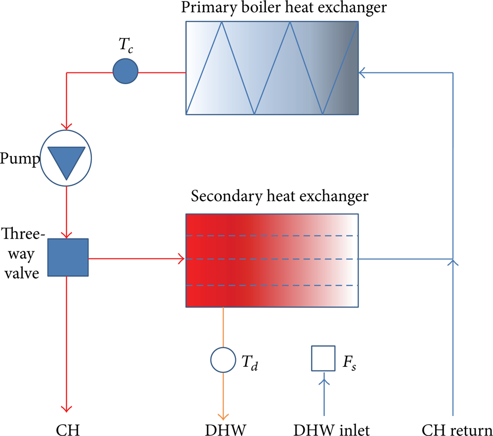
Simplified boiler scheme [10].

When the water flow rate sensor (F_s) detects a demand for domestic water, the DHW mode will be used. Here, a three-way valve will switch and the CH loop will be closed through the secondary heat exchanger; that is, during DHW operation there is no water circulation around the building, but it returns to the primary heat exchanger right after leaving the secondary. In this mode the cold water for domestic use (DHW inlet) coming from the supply system will be heated up in the secondary heat exchanger (typically plate heat exchanger) by the hot water of the central heating. The controller will define the necessary power to maintain the temperature T_d in the set point. It is worth pointing out that when T_d is being controlled the temperature T_c can vary freely.

There are two main control loops: the first one will control the temperature of the CH water leaving the primary heat exchanger and the second controller will maintain constant the temperature of the DHW at the output of the secondary heat exchanger. As it has been said, generally it is not possible to control both temperatures at the same time. It means that there will be switching between the two control loops. The supervisor will switch automatically from the CH to the DHW controller whenever the flow rate detects a demand for domestic hot water.

The control problem is different for each mode. In the CH controller the dynamics of the system are slow and the main disturbance is the ambient temperature which has a very large time scale. Furthermore, the water is driven around a closed-loop with constant flow rate.

The goal of the DHW controller is to maintain the domestic hot water T_d at the set point and reject the disturbances as fast as possible without oscillation since the performance of the controller affects directly the comfort of the user. The control of the domestic hot water temperature is much more critical than the CH controller. The conditions may change very quickly and the controller must respond fast. Here, the disturbances are mainly the water flow rate Q which is demanded and the temperature of water coming from the supply system.

The flow rate can vary drastically in a short period of time, which creates strong disturbances. In fact, one of the main challenges controlling this process is the fact that the dynamics of the system depend strongly on the demanded water flow rate, as we shall see in the following. For this reason, the focus of this paper is the robust design of the DHW controller.

Figure 2 shows the block diagram of the DHW control system. The controlled variable is the temperature T_d of the water at outlet of the secondary heat exchanger; disturbance Q is the demanded water flow rate and u is the output of the controller used to keep the temperature at the set point. This value will then be converted to the real actuator input which depends on the boiler [10].

Figure 2:

Controller in domestic hot water mode.

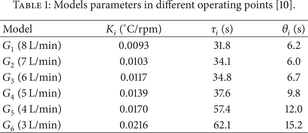
Our goal is to design the controller C_d which offers stability, fast response, and small overshoot for a whole range of water flow rate. The first step in the controller design is to obtain the system's model. Therefore, a series of open-loop experiments were carried out in order to identify models at different values of water flow rate Q In this case, we define six operating points: Q = [3, 4, 5, 6, 7, 8] L/min.

The identified systems are basically first order models in the form

G_{i} (s) = \frac{K_{i}}{τ_{i} s + 1} e^{- θ_{i} s},

(1)

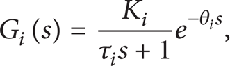
where the parameters are given in Table 1. As can be seen, the static gain K_i of the system ranges from 0.0093 up to 0.0216 while the time constant τ_i goes from 31.8's up to 62.1's. As expected using energy balance, with low flow rates the static gain of the system is higher. When the water flow rate is higher the heat transfer coefficient is also higher. This explains the smaller time constant [10].

Table 1:

Models parameters in different operating points [10].

Model	K_i(°C/rpm)	τ_i (s)	θ_i (s)

G₁ (8 L/min)	0.0093	31.8	6.2
G₂ (7 L/min)	0.0103	34.1	6.0
G₃ (6 L/min)	0.0117	34.8	6.7
G₄ (5 L/min)	0.0139	37.6	9.8
G₅ (4 L/min)	0.0170	57.4	12.0
G₆ (3 L/min)	0.0216	62.1	15.2

3. WGC Method

WGC method bases stability boundary locus approach using to obtain the stabilizing PI controller parameters region [14]. Consider the open-loop transfer function given in.

G (s) = G_{p} (s) e^{- θ s} = \frac{N (s)}{D (s)} e^{- θ s} .

(2)

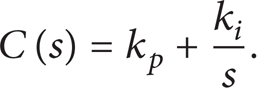
PI controller of the form is given in

C (s) = k_{p} + \frac{k_{i}}{s} .

(3)

First stage of the problem is to find the stability region which includes all the parameters of the PI controller of (3) which stabilize the given system. The closed-loop characteristic polynomial P(s) of the system, that is, the numerator of 1 + C(s)G(s), can be written as

P (s) = s D (s) + (k_{p} s + k_{i}) N (s) e^{- θ s} .

(4)

Decomposing the numerator and the denominator polynomials of G_p(s) in (2) into their even and odd parts, as well as substituting s = jω, gives

G_{p} (ω) = \frac{N_{e} (- ω^{2}) + j ω N_{o} (- ω^{2})}{D_{e} (- ω^{2}) + j ω D_{o} (- ω^{2})} .

(5)

For simplicity (–ω²) will be dropped in the following equations. Thus, the closed-loop characteristic polynomial of (4) can be written as

P (ω) = P_{R} (ω) + j P_{I} (ω),

(6)

where

P_{R} (ω) = (k_{i} N_{e} - k_{P} ω^{2} N_{o}) \cos (ω θ) + ω (k_{i} N_{o} + k_{P} N_{e}) \sin (ω θ) - ω^{2} D_{o},

(7a)

P_{I} (ω) = ω (k_{i} N_{o} + k_{P} N_{e}) \cos (ω θ) - (k_{i} N_{e} + ω^{2} k_{P} N_{o}) \sin (ω θ) + ω D_{e} .

(7b)

Then, equating the real and imaginary parts of P(ω) to zero, two equations are obtained as

Q (ω) k_{p} + R (ω) k_{i} = X (ω),

(8a)

S (ω) k_{p} + U (ω) k_{i} = Y (ω),

(8b)

where

Q (ω) = ω N_{e} \sin (ω θ) - ω^{2} N_{o} \cos (ω θ),

(9a)

S (ω) = ω N_{e} \cos (ω θ) + ω^{2} N_{o} \sin (ω θ),

(9b)

R (ω) = N_{e} \cos (ω θ) + ω N_{o} \sin (ω θ),

(9c)

U (ω) = ω N_{o} \cos (ω θ) - N_{e} \sin (ω θ),

(9d)

X (ω) = ω^{2} D_{o}, Y (ω) = - ω D_{e} .

(9e)

Finally, by solving the 2-dimensional system of (8a) and (8b) the parameters of PI controller are obtained as

k_{p} = ((ω^{2} N_{o} D_{o} + N_{e} D_{e}) \cos (ω θ) + ω (N_{o} D_{e} - N_{e} D_{o}) \sin (ω θ)) \times {(- (N_{e}^{2} + ω^{2} N_{o}^{2}))}^{- 1},

(10)

Changing ω from 0 to ∞ the stability boundary locus l(k_p,k_i,ω) is constructed in the (k_p,k_i)-plane using (10) and (11). As a special case, a real root can cross over the imaginary axis at s = 0. Thus, a real root boundary is obtained by substituting s = 0 in P(s) of (4). Therefore, this special boundary is determined as

k_{i} = (ω^{2} (N_{o} D_{e} - N_{e} D_{o}) \cos (ω θ) - ω (N_{e} D_{e} + ω^{2} N_{o} D_{o}) \sin (ω θ)) \times {(- (N_{e}^{2} + ω^{2} N_{o}^{2}))}^{- 1} .

(11)

The stability boundary locus and the real root boundary divide the parameter plane (k_p,k_i) into stable and unstable regions. The stable region can be obtained by choosing a test point within each region. The characteristic equation belonging to an arbitrary point in the stable region has no right-half of the s-plane (RHP) roots until the characteristic polynomial of any point in the unstable region has a certain number of RHP roots.

3.1. Example

Consider the transfer function of the first order plus time delay (FOPTD) system has the form

k_{i} = 0 .

(12)

Here, the aim is to obtain all stabilizing values of k_p and k_i that make the closed-loop system in Figure 1 stable. The characteristic equation of the control system is derived as

G (s) = \frac{1}{s + 1} e^{- s} .

(13)

By applying the stabilization procedure, the k_p and k_i values for the stability boundary locus are obtained as

P (s) = s^{2} + s + (k_{P} s + k_{i}) e^{- s} .

(14)

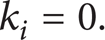
Figure 3 shows the stability boundary locus for a range of frequency ω(0, 2.19) and the real root boundary line. It can be observed from this figure that the parameter plane is divided into four regions, namely, R₁, R₂, R₃, and R₄. By choosing one arbitrary test point in each region, the stability region which is the shaded region (R₂) shown in Figure 3 can be determined. Figure 4 shows more clearly R₂ for all stabilizing values of k_p and k_i. In this figure, the stability boundary locus is computed for the range of ω[0,ω_i]. Equating (11) to (12), the intersection frequency ω_i is calculated as 2.03.

Figure 3:

Stability boundaries of the FOPTD system.

Figure 4:

Stability region.

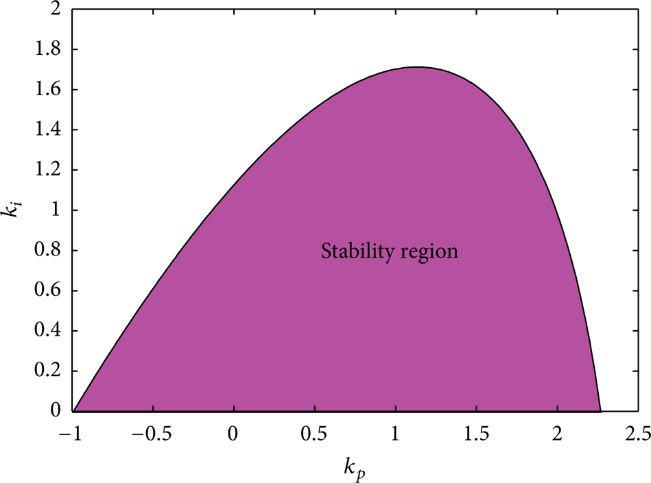
The plotting of the stability boundary locus is based on the calculation of (k_p,k_i) pairs at each ω value as given in (10) and (11) and then the connection of each (k_p,k_i) point together in the parameter plane. The point based stability boundary locus for the FOPTD system in (13) is shown in Figure 5. In this figure, each (k_p,k_i) point is marked by changing ω from 0 to 2.03 in steps of 0.03. It is seen from this figure that the distance between each points is not the same. The points are closely spaced at small ω values. With increasing the values of ω they become distant and then tighten around the peak point of stability boundary locus and finally it unwraps when reached the stability boundary locus to the real root boundary.

Figure 5:

(k_p,k_i) points constituting the stability boundary locus depending on ω values.

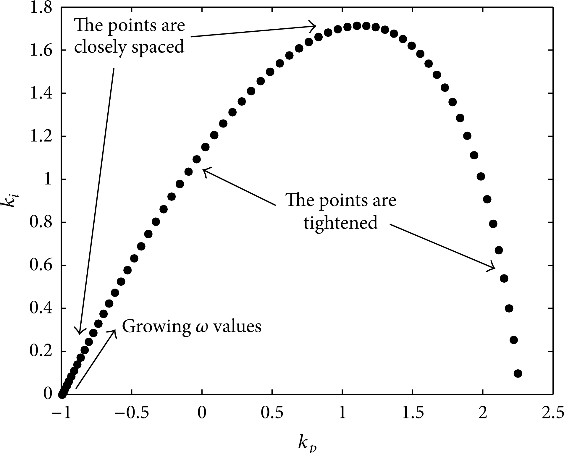
This locus enclosing the stability region consists of n points of which the coordinates are defined as (k_p1,k_i1), (k_p2,k_i2), (k_p3,k_i3), …, (k_pn,k_in). However, the real root boundary, k_i = 0, which limits the stability boundary locus for obtaining the stability region does not depend on ω. For this line, the projections of the points in the stability boundary locus are considered as shown in Figure 6. In this case, the coordinates of the projection points are (k_p1, 0), (k_p2, 0), and (k_p3, 0), …, (k_pn, 0).

Figure 6:

The coordinates of (k_p,k_i) points constituting the stability boundary locus and their projections for the real root boundary line for ω(0, 0.12).

As a result of combining the points of stability boundary locus and real root boundary line, the weighted geometrical center (k_pw,k_iw) of the stability region is obtained easily as follows:

\begin{matrix} k_{P} = ω \sin ω - \cos ω, \\ k_{i} = ω \sin ω + ω^{2} \cos ω . \end{matrix}

(15)

Thus, the weighted geometrical center using (16) can be found precisely. This method gives a simple PI tuning rule which provides a good transient performance for the time delay systems [13].

An algorithm calculating the WGC controller of any system with time delay is presented in Figure 7. The algorithm calculates WGC controller for open-loop transfer function and time delay of the system. In other words, it obtains the stabilizing PI controller parameters region for aforementioned system and calculates the weighted geometric center controller for this region in response to entering the coefficients of numerator and denominator polynomials (a₁,a₂, …, a_m and b₁,b₂, …, b_n) of open-loop transfer function and time delay in the system by the user. According to this, the characteristic equation of closed-loop system is obtained at the 1st step. The s = jω transformation is made at the 2nd step. The imaginer terms of characteristic equation are separated from reel terms and two different equations are obtained at the 3rd step. This operation is realized by differentiating the characteristic equation with respect to k_p and k_i. The equation system is solved in a cycle dependent on a frequency (ω) and the root pair (root₁ and root₂) in response to each frequency is calculated at the 4th step. In case the second root (root₂) receives a value less than zero, the cycle stops the calculation. Likewise, the points of boundary locus of the stability region are obtained. In the final step, weighted geometric center controller is obtained by evaluating the coordinate values of the points in (16) obtained along the cycle. The Matlab 2012b codes of proposed algorithm are given in Algorithm 1.

Algorithm 1:

Matlab 2012b codes of the PI design algorithm.

Figure 7:

PI tuning algorithm.

4. PI Controller Design

While the design of a PI controller that matches the specifications for a single operating point seems to be trivial, finding a fixed controller which works properly in all operating points might not be such a simple task. In order to solve this problem, two numerical methods are presented. Firstly, WGC based robust PI control is designed and then WGC based gain scheduling PI controller is designed.

4.1. WGC Based Robust PI Controller

Proposed robust PI design method is based on calculating the joint stabilizing control parameters region and its WGC point by means of the calculating algorithm presented in Section 3. The stabilizing control parameter regions and its WGC points obtained for six different systems given in Table 1 are shown in Figure 8 and Table 2, respectively. As it is expected, increase in time delay limits the stabilizing controller parameter area. Accordingly, joint stability region corresponding to different values of the time delay is the most interior region. For this reason, the WGC controller of the most interior area remaining in the entire stability regions between the considered time delay value ranges is selected as a robust PI controller. The parameters of this controller are k_p = 110.5 and k_i = 2.66.

Table 2:

The WGC controller parameters corresponding to different time delay values.

T _D	k_p	k_i

G₁ (8 L/min)	323.6	17.95
G₂ (7 L/min)	327.7	18.02
G₃ (6 L/min)	261.6	13.30
G₄ (5 L/min)	158.0	6.21
G₅ (4 L/min)	165.3	4.80
G₆ (3 L/min)	110.5	2.66

Figure 8:

Stability regions in accordance with different time delay values.

4.2. WGC Based Gain Scheduling PI Controller

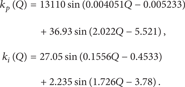
To obtain the gain scheduling PI controller, by using the values given in Table 2, the controller parameters are obtained as a function of time delay by means of Matlab Curve Fitting Toolbox. In (17), the expressions of controller parameters of k_p and k_i according to water flow rate (Q) are given, respectively. In Figure 9, the change of fitted k_p(Q) and k_i(Q) functions corresponding to water flow rate is shown. Here, it is seen that the fitted curve provides good precision:

\begin{matrix} k_{p w} = \frac{1}{n} \sum_{j = 1}^{n} k_{p j}, \\ k_{i w} = \frac{1}{2 n} \sum_{j = 1}^{n} k_{i j} . \end{matrix}

(16)

Figure 9:

Change of controller parameters with water flow rate.

4.3. Set Point Weighting

WGC based PI design method is usually based on specification of the desired closed-loop transfer function for load/disturbance changes. Consequently, the resulting WGC controllers tend to perform well for load/disturbance responses, but the set point change might not be satisfactory. Chen and Seborg [15] employed a set point weighting, which was originally proposed by Åström and Bell [16], to reduce large overshoot for PID controllers. A set point weighting for PI control structure is

\begin{matrix} k_{p} (Q) = 13110 \sin (0.004051 Q - 0.005233) + 36.93 \sin (2.022 Q - 5.521), \\ k_{i} (Q) = 27.05 \sin (0.1556 Q - 0.4533) + 2.235 \sin (1.726 Q - 3.78) . \end{matrix}

(17)

where b is the set point weighting coefficient and 0 ≤ b ≤ 1. Furthermore, Chen and Seborg [15] and Pai et al. [17] also pointed out that the large overshoot for the set point response of the PI/PID controller can normally be eliminated by setting b = 0.5. Good compromising between overshoot and settling time performances is generally obtained by setting b = 0.5 [15, 17]. Accordingly, the set point weighting with b = 0.5 is also employed for the proposed PI settings throughout the present study.

5. Simulations

Six different values of the water flow rate are used to demonstrate the performance of the proposed approaches in this section. Throughout the simulation, the PI and gain scheduling PI control algorithms with set point weighting as shown in Figures 10(a) and 10(b), respectively, are employed. Accordingly, PI controller parameters are scheduled by using the water flow rate which can be measured in real time.

Figure 10:

Control structures. (a) PI controller structure. (b) Gain scheduling PI controller structure.

In addition, a step change with magnitude 25 is introduced either in load disturbance (L) or in set point (r) for the simulation studies. Performance criterions of the closed-loop response for each case is evaluated by settling time (t_s), percent overshoot (OS%), maximum peak height (M_p), and maximum absolute value of the control signal ( ${| u |}_{\max}$ ). For both load disturbance and set point changes, the settling time (t_s) here is defined as the error to come within some prescribed band of the steady-state value (i.e., zero) and remain in this band. The band limits ± 0.02 are chosen in this study. Furthermore, the set point weighting coefficient b = 0.5 is also chosen for the present paper. In order to evaluate the general performance of closed-loop response for each case, a general evaluating function (J) is defined by using of scaled performance criterions. The function is given in (19). According to this function, the performance criterions are equally weighted in general evaluating function:

y (t) = k_{p} [b r (t) - T_{d} (t)] + k_{i} \int_{0}^{t} [r (τ) - T_{d} (τ)] d τ,

(18)

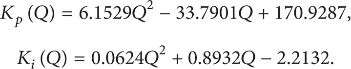
Throughout the simulations, robust and gain scheduling PI controllers given in [10] are used for comparison. Oliveire and Karimi's robust control settings are k_p = 103.2 and k_i = 1.584 [10]. Moreover, Oliveire and Karimi's gain scheduling control expressions are given in [10]

J = \frac{1}{3} (scaled t_{s}) + \frac{1}{3} (scaled M_{p} or OS %) + \frac{1}{3} (scaled {| u |}_{\max}) .

(19)

\begin{matrix} K_{p} (Q) = 6.1529 Q^{2} - 33.7901 Q + 170.9287, \\ K_{i} (Q) = 0.0624 Q^{2} + 0.8932 Q - 2.2132 . \end{matrix}

(20)

In the first stage of the simulations, it is considered that a PI controller which should guarantee robust stability and load disturbance rejection performances for all operating points is presented by models G₁ to G₆ in Table 1. Typical response curves based on the proposed settings and that of Oliveire and Karimi to a load disturbance change with magnitude 25 are shown in Figure 11. Moreover, numerical values of the performance criterions and its scaled values together with the numerical values of general evaluating function (J) are given in Table 3. It is clear that the proposed scheduling method can achieve faster response than that of Oliveire and Karimi. In all other cases except last case (G₆), the proposed gain scheduling controller is superior according to J function. In the case of G₆, best controller in the way of minimizing the function J is the proposed robust controller. Note that the proposed robust controller is the WGC controller calculated for the case of G₆.

Table 3:

Numerical values of the performance criterions for disturbance.

Model	Method	t_s	Scaled t_s	M _p	Scaled M_p	${\| u \|}_{\max}$	Scaled u_max	J

G ₁	Proposed (gain scheduling)	50.6558	0.1029	0.0625	0.6021	32.7146	1.0000	0.5627
	Proposed (robust)	283.3529	0.5757	0.0974	0.9383	24.9996	0.7642	0.7518
	Oliveire and Karimi (gain scheduling)	150.5503	0.3059	0.0654	0.6301	26.3503	0.8055	0.5747
	Oliveire and Karimi (robust)	492.1735	1.0000	0.1038	1.0000	24.9430	0.7624	0.9116

G ₂	Proposed (gain scheduling)	67.2276	0.1444	0.0634	0.5849	33.1928	1.0000	0.5706
	Proposed (robust)	266.6698	0.5726	0.1013	0.9345	24.9999	0.7532	0.7459
	Oliveire and Karimi (gain scheduling)	155.7292	0.3344	0.0725	0.6688	25.3021	0.7623	0.5826
	Oliveire and Karimi (robust)	465.6869	1.0000	0.1084	1.0000	24.9633	0.7521	0.9082

G ₃	Proposed (gain scheduling)	74.2277	0.1704	0.0776	0.6616	32.6121	1.0000	0.6045
	Proposed (robust)	249.3930	0.5724	0.1103	0.9403	25.0000	0.7666	0.7522
	Oliveire and Karimi (gain scheduling)	168.6857	0.3872	0.0879	0.7494	25.0713	0.7688	0.6288
	Oliveire and Karimi (robust)	435.6812	1.0000	0.1173	1.0000	24.9777	0.7659	0.9127

G ₄	Proposed (gain scheduling)	75.2285	0.1918	0.1162	0.8488	31.6540	1.0000	0.6734
	Proposed (robust)	222.0267	0.5661	0.1315	0.9606	25.0000	0.7898	0.7644
	Oliveire and Karimi (gain scheduling)	194.2487	0.4952	0.1187	0.8671	26.5127	0.8376	0.7260
	Oliveire and Karimi (robust)	392.2342	1.0000	0.1369	1.0000	24.9903	0.7895	0.9205

G ₅	Proposed (gain scheduling)	138.4716	0.4045	0.1208	0.8401	31.8106	1.0000	0.7407
	Proposed (robust)	171.3050	0.5004	0.1372	0.9541	27.3230	0.8589	0.7634
	Oliveire and Karimi (gain scheduling)	267.4137	0.7811	0.1303	0.9061	25.7304	0.8089	0.8237
	Oliveire and Karimi (robust)	342.3481	1.0000	0.1438	1.0000	24.9993	0.7859	0.9193

G ₆	Proposed (gain scheduling)	173.8562	0.2971	0.1729	0.9713	31.0657	0.9869	0.7443
	Proposed (robust)	163.2802	0.2791	0.1724	0.9685	31.4775	1.0000	0.7417
	Oliveire and Karimi (gain scheduling)	585.0799	1.0000	0.1707	0.9590	25.3844	0.8064	0.9126
	Oliveire and Karimi (robust)	306.9059	0.5246	0.1780	1.0000	26.4397	0.8400	0.7803

Figure 11:

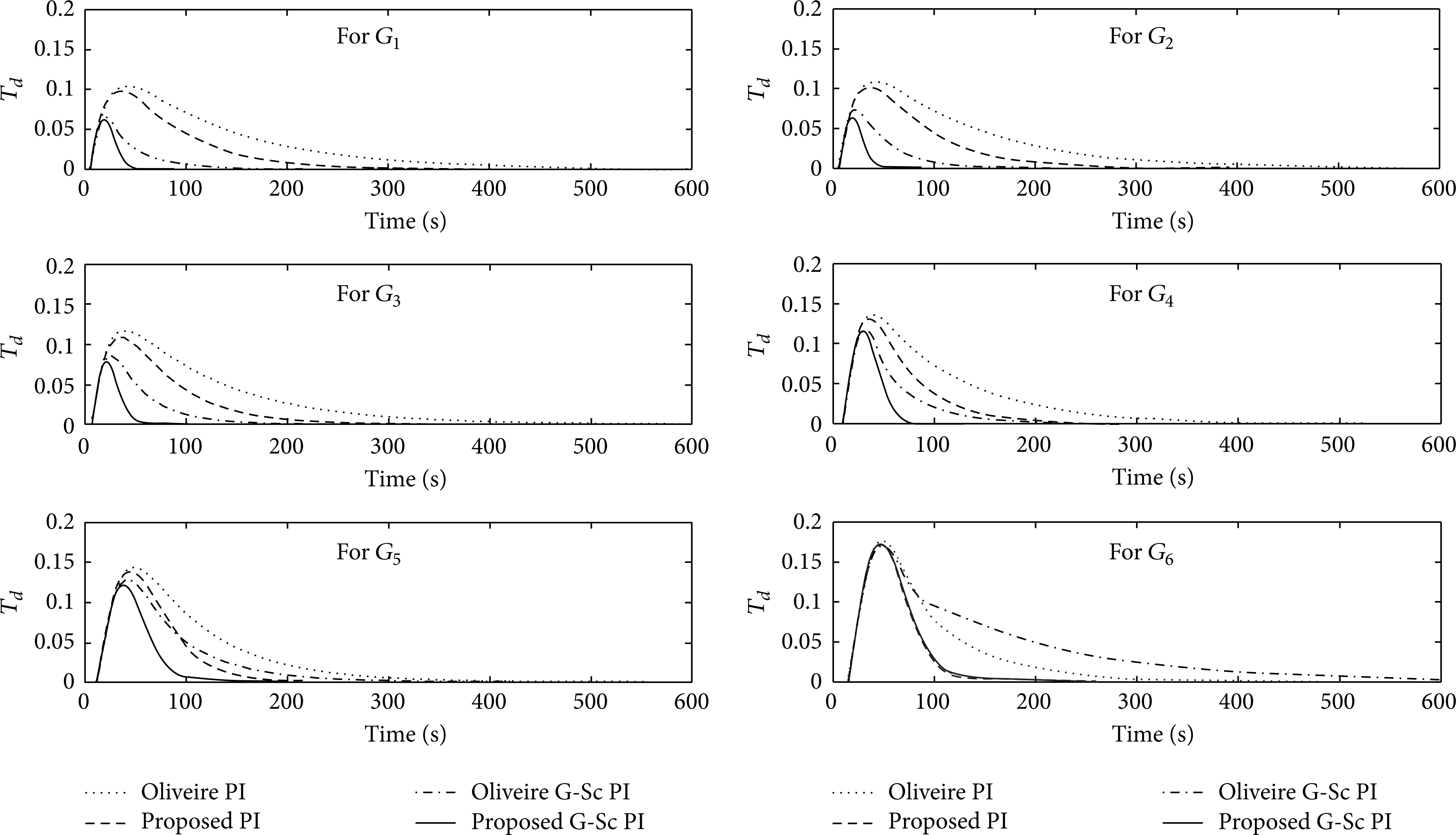
Comparison of disturbance responses.

In the second stage of the simulations, closed-loop response curves of the proposed PI settings and that of Oliveire and Karimi for a set point change with magnitude of 25 are shown in Figure 12. Furthermore, numerical values of the performance criterions and their scaled values together with the numerical values of general evaluating function (J) are given in Table 4. Figure 12 and Table 4 indicate that proposed gain scheduled method is very good for set point changes in all operating conditions, especially for lower settling time. However, according to values of the function J, in all other cases except last case (G₅), the proposed robust controller is superior. In case of G₅, best controller in the way of minimizing the function J is the proposed gain scheduling controller. Note that the maximum control signal value calculated by the proposed controllers is considerably lower than that of Oliveire and Karimi. It can be seen in simulation results that the most critical conditions in the robust control design are those with small water flow rate because of the higher gains and time constants. This means that boundary of feasibility for the robust controller design is defined by the models in those conditions. It has to be stated that once a WGC based robust controller is designed it will respect this boundary (see Figure 8). There are similar findings in that of the study of Oliveire and Karimi. However, these results are too conservative in other operating points with higher flow rates, which deteriorates the performance. If a gain scheduled controller is used, it will respect the constraints by the most critical models and at the same time will have room for performance improvement in different conditions.

Table 4:

Numerical values of the performance criterions for set point changes.

Model	Method	t_s	Scaled t_s	OS	Scaled OS	${\| u \|}_{\max}$	Scaled u_max	J

G ₁	Proposed (gain scheduling)	38.3058	0.1067	3.1415	0.5816	6853.5	0.7839	0.4907
	Proposed (robust)	228.0458	0.6351	0	0	2688.1	0.3075	0.3142
	Oliveire and Karimi (gain scheduling)	35.4055	0.0986	5.4013	1.0000	8742.5	1.0000	0.6995
	Oliveire and Karimi (robust)	359.0767	1.0000	0	0	2825.4	0.3232	0.4410

G ₂	Proposed (gain scheduling)	34.9212	0.1063	2.7257	1.0000	6845.6	0.9834	0.6965
	Proposed (robust)	210.8267	0.6420	0	0	2427.2	0.3487	0.3302
	Oliveire and Karimi (gain scheduling)	27.5221	0.0838	1.2085	0.4434	6961.1	1.0000	0.5090
	Oliveire and Karimi (robust)	328.3709	1.0000	0	0	2817.4	0.4047	0.4682

G ₃	Proposed (gain scheduling)	28.7216	0.0968	1.8632	1.0000	5498.5	0.9740	0.6902
	Proposed (robust)	195.9766	0.6604	0	0	2136.7	0.3785	0.3463
	Oliveire and Karimi (gain scheduling)	32.0876	0.1081	0.2851	0.1530	5645.0	1.0000	0.4203
	Oliveire and Karimi (robust)	296.7630	1.0000	0	0	2845.2	0.5040	0.5013

G ₄	Proposed (gain scheduling)	57.9169	0.2307	2.5680	0.4244	3652.9	0.7565	0.4705
	Proposed (robust)	173.5156	0.6913	0	0	2052.7	0.4251	0.3721
	Oliveire and Karimi (gain scheduling)	52.1205	0.2076	6.0510	1.0000	4828.8	1.0000	0.7358
	Oliveire and Karimi (robust)	251.0162	1.0000	0	0	2967.9	0.6146	0.5381

G ₅	Proposed (gain scheduling)	55.3583	0.4054	0.0441	0.0151	3443.9	0.8477	0.4227
	Proposed (robust)	107.1685	0.7848	0.0704	0.0241	2269.9	0.5587	0.4558
	Oliveire and Karimi (gain scheduling)	72.9943	0.5345	2.9218	1.0000	4062.5	1.0000	0.8447
	Oliveire and Karimi (robust)	136.5619	1.0000	0	0	3055.0	0.7520	0.5839

G ₆	Proposed (gain scheduling)	123.3720	0.3830	0	0	2372.7	0.6752	0.3527
	Proposed (robust)	68.0604	0.2113	0.6100	0.1059	2422.0	0.6893	0.3355
	Oliveire and Karimi (gain scheduling)	322.1192	1.0000	1.5376	0.2670	3513.9	1.0000	0.7556
	Oliveire and Karimi (robust)	84.8239	0.2633	5.7586	1.0000	3181.8	0.9055	0.7229

Figure 12:

Comparison of set point responses.

6. Conclusions

In this paper two methodologies to robust PI controller design for boiler temperature control systems are presented. Important qualifications of these PI design approaches are that the resulting parameters are numerically calculated without turning to any graphical method or iterative optimization process and that they guarantee the stability of the closed-loop. With the proposed gain scheduling approach it has been possible to cope with large variations in the operating conditions providing good performance for the whole range of demanded flow rate. However, requirement for one more sensor for sensing the water flow rate is disadvantageous for the scheduling method. Alternatively, an estimator of the water flow rate could be implemented to provide the information. Such estimator would need the information regarding the temperature of the incoming water. This is economically advantageous over the flow-meter solution since normally temperature sensors are cheaper than flow-meters. The results of the comparative simulation studies show that the proposed scheduling method will provide successful results for boiler systems where the water flow rate can be observed or estimated.

Conflict of Interests

The author declares that there is no conflict of interests regarding the publication of this paper.

References

Toscano

, “Robust synthesis of a PID controller by uncertain multimodel approach,” Information Sciences, vol. 177, no. 6, pp. 1441–1451, 2007.

Chiu

M. S.

, and Wang

Q. G.

, “Robust PID controller design via LMI approach,” Journal of Process Control, vol. 12, no. 1, pp. 3–13, 2002.

Nyström

R. H.

Sandström

K. V.

Gustafsson

T. K.

, and Toivonen

H. T.

, “Multimodel robust control of nonlinear plants: a case study,” Journal of Process Control, vol. 9, no. 2, pp. 135–150, 1999.

Karimi

and Galdos

, “Fixed-order H_∞ controller design for nonparametric models by convex optimization,” Automatica, vol. 46, no. 8, pp. 1388–1394, 2010.

Onat

Kucukdemiral

I. B.

Sivrioglu

, and Yuksek

, “LPV model based gain-scheduling controller for a full vehicle active suspension system,” JVC/Journal of Vibration and Control, vol. 13, no. 11, pp. 1629–1666, 2007.

Onat

Kucukdemiral

I. B.

Sivrioglu

Yuksek

, and Cansever

, “LPV gain-scheduling controller design for a nonlinear quarter-vehicle active suspension system,” Transactions of the Institute of Measurement and Control, vol. 31, no. 1, pp. 71–95, 2009.

Blanchett

T. P.

Kember

G. C.

, and Dubay

, “PID gain scheduling using fuzzy logic,” ISA Transactions, vol. 39, no. 3, pp. 317–325, 2000.

Zhao

Z. Y.

Tomizuka

, and Isaka

, “Fuzzy gain scheduling of PID controllers,” IEEE Transactions on Systems, Man and Cybernetics, vol. 23, no. 5, pp. 1392–1398, 1993.

Leith

D. J.

and Leithead

W. E.

, “Survey of gain-scheduling analysis and design,” International Journal of Control, vol. 73, no. 11, pp. 1001–1025, 2000.

10.

Oliveire

and Karimi

, “Robust and gain-scheduled PID controller design for condensing boilers by linear programing,” in Proceedings of the 2nd International Federation of Automatic Conference on Advanced in PID Control (IFAC '12), pp. 335–340, Brescia, Italy, 2012.

11.

Karimi

Kunze

, and Longchamp

, “Robust controller design by linear programming with application to a double-axis positioning system,” Control Engineering Practice, vol. 15, no. 2, pp. 197–208, 2007.

12.

Kunze

Karimi

, and Longchamp

, “Gain scheduled controller design by linear programming,” in Proceedings of the European Control Conference, pp. 5432–5438, 2007.

13.

Onat

, “A new concept on PI design for time delay systems: weighted geometrical center,” International Journal of Innovative Computing, Information and Control, vol. 9, pp. 1539–1556, 2013.

14.

Tan

Kaya

, and Atherton

D. P.

, “Computation of stabilizing PI and PID controllers,” in Proceedings of IEEE Conference on Control Applications (CCA '03), pp. 876–881, Istanbul, Turkey, June 2003.

15.

Chen

and Seborg

D. E.

, “PI/PID controller design based on direct synthesis and disturbance rejection,” Industrial and Engineering Chemistry Research, vol.41, no. 19, pp. 4807–4822, 2002.

16.

Åström

K. J.

and Bell

R. D.

, “Drum-boiler dynamics,” Automatica, vol. 36, no. 3, pp. 363–378, 2000.

17.

Pai

N. S.

Chang

S. C.

, and Huang

C. T.

, “Tuning PI/PID controllers for integrating processes with deadtime and inverse response by simple calculations,” Journal of Process Control, vol. 20, no 6, pp 726–733, 2010

WGC Based Robust and Gain Scheduling PI Controller Design for Condensing Boilers

Abstract

1. Introduction

2. System Description

3. WGC Method

3.1. Example

4. PI Controller Design

4.1. WGC Based Robust PI Controller

4.2. WGC Based Gain Scheduling PI Controller

4.3. Set Point Weighting

5. Simulations

6. Conclusions

Conflict of Interests

References