Monitoring Technology for Vehicle Loading Status Based on the Analysis of Suspension Vibration Characters

Abstract

Monitoring and early warning of vehicle risk status was one of the key technologies of transportation security, and real-time monitoring load status could reduce the transportation accidents effectively. In order to obtain vehicle load status information, vehicle characters of suspension were analyzed and simulated under different working conditions. On the basis of this, the device that can detect suspension load with overload protection structure was designed and a method of monitored vehicle load status was proposed. The monitoring platform of vehicle load status was constructed and developed for a FAW truck and system was tested on level-A road and body twist lane. The results show that the measurement error is less than 5% and horizontal centre-of-mass of vehicle was positioned accurately. The platform enables providing technical support for the real-time monitoring and warning of vehicles risk status in transit.

1. Introduction

Highway transportation accidents are frequent in recent years; direct costs of property damages and the number of casualties in the serious accident are huge. The Accident Analysis Reporting System reported that commercial truck traffic accidents accounted for 29.9% of all country's accidents in 2010, the number of incidents that more than five people were killed in an accident is 152, and the safety problem of highway transportation has become one of the problems urgently to be solved. Nonstandard loading including overload, partial load and so forth causes degrading performance of vehicle braking and steering stability [1–4]; it is one of the important reasons leading to traffic accidents. The practices of monitoring the vehicle load status effectively reduce the transportation accidents, and acquisition of tire vertical load information provides technical support for study on braking distance prediction and vehicle stability during cornering.

The companies usually use van semitrailer to transport Cargos in developed countries; this way of freight is relatively formal, but in developing countries, it still keeps the way of binding goods in transportation. Some companies and individuals still use light truck to transport in shortdistance. Terms of nonstandard transport led to vehicle load status abnormalities [5]. Risk load status basically is divided into two types: one is static load abnormalities, including partial loading and overloading which are caused by irregular loading; the other is the dynamic load abnormalities including Cargo sliding and coming off in special circumstances.

The traditional device detection of vehicle load includes static axle load meter and weigh-in-motion (WIM) [6]; WIM is a measurement that obtains the load values by measuring tire vertical force based on resilience sensors. It is used to measure vehicle tire vertical force in the condition of the specific location and low speed running; these measurement methods are offline rather than online. Given the limitations of measuring time and place, in order to obtain dynamic load of vehicles, many researchers have made a series of studies. In the study by Leimbach and Gabriel [7], vehicle mass center height was calculated by measuring and comparing tire speed; the method was applied to research vehicle rollover control strategy. Vahidi et al. [8] studied algorithm of real-time estimating vehicle load and road slope using recursive least squares with forgotten factor. This method is mainly used to estimate the vehicle dynamic load relative to the ground. In the study by Shimp III [9] and Kewlani et al. [10], estimation algorithm of vehicle sprung mass was put forward based on the polynomial chaos theory. This method is suitable for vehicles running at low speed, and the calculation is heavy and real-time performance is weak. In the study by Pence et al. [11] and Solmaz et al. [12, 13], data of vehicle operation parameters (lateral deceleration, yaw rate, wheel angle and longitudinal speed) was collected by multiple sensors and input to a set of simplified models of the vehicle, comparing with real vehicle measurement results; minimum relative error of the model parameters was used as vehicle current state. This study realized real-time estimating centroid position of dynamic load, but the method of calculation is too heavy, requiring that computing power of vehicle terminal is higher and system implementation is difficult.

In this study, dynamic characteristics of vehicle suspension were analyzed and studied by setting up vibration travel. Vehicle load detection device with overload protection structure was designed based on displacement sensor; sensor signal was collected and processed by SCM; the load values were displayed on the vehicle computer and information was provided to the driver in real-time. Designed load detection device was simply installed in the car and the amount of data collection and calculation is reasonable. The experiment shows that the platform has a high calculation speed and a good performance in real-time. Vehicle load statues were monitored conveniently and accurately; this method adapts to a variety of conditions for driving environment.

2. Suspension Dynamic Model[14–18]

Vehicle enroute vibrates due to excitation from rotating parts as engine, transmission system, and the wheel; road roughness is the basic input of vehicle vibration. Heavy truck generally uses the rigid axle suspension as a damping structure. Leaf spring as the elastic component can play the role of steering mechanism and absorb the vibration. In order to analyze the characteristics of suspension, structures were simplify and the independent suspension vibration model was established.

2.1. Suspension Vibration Model

Automobile is a complicated vibration system, to obtain the relative displacement between vehicle body and suspension, simplify rear bridge structure of nonindependent suspension, and establish vehicle vibration model as shown in Figure 1.

Figure 1:

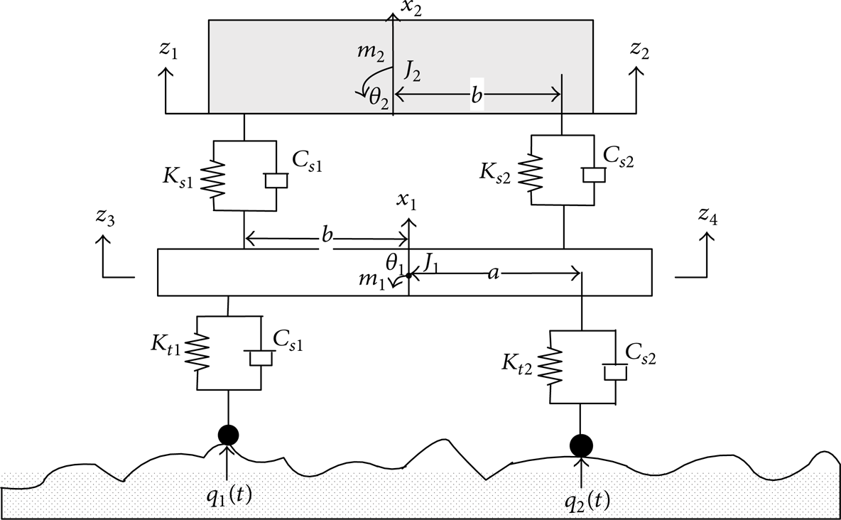
Vehicle vibration model.

According to Newton's second law, differential equation of model was establish as

$\begin{array}{c}{m}_{\mathrm{1}}{\ddot{x}}_{\mathrm{1}}\left(t\right)+K_t\left[z_{\mathrm{1}}\left(t\right)+z_{\mathrm{2}}\left(t\right)\right]+C_t\left[{\dot{z}}_{\mathrm{1}}\left(t\right)+{\dot{z}}_{\mathrm{2}}\left(t\right)\right]-K_s\left[z_{\mathrm{3}}\left(t\right)+z_{\mathrm{4}}\left(t\right)\right]-C_s\left[{\dot{z}}_{\mathrm{3}}\left(t\right)+{\dot{z}}_{\mathrm{4}}\left(t\right)\right]=\mathrm{0},\\ J_{\mathrm{1}}{\ddot{\theta }}_{\mathrm{1}}+a·K_t\left[z_{\mathrm{2}}\left(t\right)-z_{\mathrm{1}}\left(t\right)\right]+a·C_t\left[{\dot{z}}_{\mathrm{2}}\left(t\right)-{\dot{z}}_{\mathrm{1}}\left(t\right)\right]+c·K_s\left[z_{\mathrm{3}}\left(t\right)-z_{\mathrm{4}}\left(t\right)\right]+c·C_s\left[{\dot{z}}_{\mathrm{3}}\left(t\right)-{\dot{z}}_{\mathrm{4}}\left(t\right)\right]=\mathrm{0},\\ m_{\mathrm{2}}{\ddot{x}}_{\mathrm{2}}\left(t\right)+K_s\left[z_{\mathrm{3}}\left(t\right)+z_{\mathrm{4}}\left(t\right)\right]+C_s\left[{\dot{z}}_{\mathrm{3}}\left(t\right)+{\dot{z}}_{\mathrm{4}}\left(t\right)\right]=\mathrm{0},\\ J_{\mathrm{2}}{\ddot{\theta }}_{\mathrm{2}}+b·K_s\left[z_{\mathrm{4}}\left(t\right)-z_{\mathrm{3}}\left(t\right)\right]+b·C_s\left[{\dot{z}}_{\mathrm{4}}\left(t\right)-{\dot{z}}_{\mathrm{3}}\left(t\right)\right]=\mathrm{0},\end{array}$

(1)

where z1 and z₂ are amount of tire vertical deformations, z3 and z4 amount of suspension elastic element deformations, and z1, z2, z3, and z4 can be expressed by vertical displacement of the vehicle body x1 and suspension structure x2 as follows:

${\left[\begin{array}{cccc}{z}_{\mathrm{1}}& z_{\mathrm{2}}& z_{\mathrm{3}}& z_{\mathrm{4}}\end{array}\right]}^T={\left[\begin{array}{cccc}\begin{array}{c}\mathrm{1}\\ \mathrm{0}\end{array}& \begin{array}{c}\mathrm{1}\\ \mathrm{0}\end{array}& \begin{array}{c}-\mathrm{1}\\ \mathrm{1}\end{array}& \begin{array}{c}-\mathrm{1}\\ \mathrm{1}\end{array}\end{array}\right]}^T\left[\begin{array}{c}{x}_{\mathrm{1}}\\ x_{\mathrm{2}}\end{array}\right]+{\left[\begin{array}{cccc}\begin{array}{c}a\\ \mathrm{0}\end{array}& \begin{array}{c}a\\ \mathrm{0}\end{array}& \begin{array}{c}c\\ -b\end{array}& \begin{array}{c}-c\\ b\end{array}\end{array}\right]}^T\left[\begin{array}{c}{\theta }_{\mathrm{1}}\\ {\theta }_{\mathrm{2}}\end{array}\right]+{\left[\begin{array}{cccc}\begin{array}{c}-\mathrm{1}\\ \mathrm{0}\end{array}& \begin{array}{c}\mathrm{0}\\ -\mathrm{1}\end{array}& \begin{array}{c}\mathrm{0}\\ \mathrm{0}\end{array}& \begin{array}{c}\mathrm{0}\\ \mathrm{0}\end{array}\end{array}\right]}^T\left[\begin{array}{c}{q}_{\mathrm{1}}\\ q_{\mathrm{2}}\end{array}\right].$

(2)

Differential equation (1) was simplified to matrix form as

$M\ddot{X}+C\dot{X}+KX=C_q\dot{Q}+K_{q}Q,$

(3)

where M, C, K, C _q , and K _q are coefficient matrices in the equation as follows:

$\begin{array}{c}M=\left[\begin{array}{cccc}{m}_{\mathrm{1}}& \mathrm{0}& \mathrm{0}& \mathrm{0}\\ \mathrm{0}& J_{\mathrm{1}}& \mathrm{0}& \mathrm{0}\\ \mathrm{0}& \mathrm{0}& m_{\mathrm{2}}& \mathrm{0}\\ \mathrm{0}& \mathrm{0}& \mathrm{0}& J_{\mathrm{2}}\end{array}\right];\\ Q={\left[\begin{array}{cccc}{q}_{\mathrm{1}}\left(t\right)& q_{\mathrm{2}}\left(t\right)& \mathrm{0}& \mathrm{0}\end{array}\right]}^T;\\ X={\left[\begin{array}{cccc}{x}_1\left(t\right)& {\theta }_t\left(t\right)& x_2\left(t\right)& {\theta }_t\left(t\right)\end{array}\right]}^T;\\ C=\mathrm{2}\times \left[\begin{array}{cccc}{C}_t+C_s& -C_s& \mathrm{0}& \mathrm{0}\\ -C_s& C_s& \mathrm{0}& \mathrm{0}\\ \mathrm{0}& \mathrm{0}& C_t·a^{\mathrm{2}}+C_s·c^{\mathrm{2}}& -C_s·b·c\\ \mathrm{0}& \mathrm{0}& -C_s·b·c& C_s·b^{\mathrm{2}}\end{array}\right];\\ K=\mathrm{2}\times \left[\begin{array}{cccc}{K}_t+K_s& -K_s& \mathrm{0}& \mathrm{0}\\ -K_s& K_s& \mathrm{0}& \mathrm{0}\\ \mathrm{0}& \mathrm{0}& K_t·a^{\mathrm{2}}+K_s·c^{\mathrm{2}}& -K_s·bc\\ \mathrm{0}& \mathrm{0}& -K_s·b·c& K_s·b^{\mathrm{2}}\end{array}\right];\\ C_q=\left[\begin{array}{cccc}{C}_t& C_t& \mathrm{0}& \mathrm{0}\\ \mathrm{0}& \mathrm{0}& \mathrm{0}& \mathrm{0}\\ -C_t·a& C_t·a& \mathrm{0}& \mathrm{0}\\ \mathrm{0}& \mathrm{0}& \mathrm{0}& \mathrm{0}\end{array}\right];\\ K_q=\left[\begin{array}{cccc}{K}_t& K_t& \mathrm{0}& \mathrm{0}\\ \mathrm{0}& \mathrm{0}& \mathrm{0}& \mathrm{0}\\ -K_t·a& K_t·a& \mathrm{0}& \mathrm{0}\\ \mathrm{0}& \mathrm{0}& \mathrm{0}& \mathrm{0}\end{array}\right].\end{array}$

(4)

2.2. Road Surface Roughness

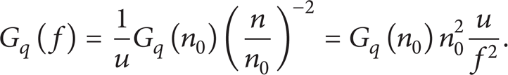
Road roughness as the input of vehicle vibration model is curve function of road vertical section; it mainly uses the road power spectral density to describe the statistical properties [19, 20]. The international organization for standardization put forward draft of road roughness expression method in document ISO/TC 108/SC2N67 in 1984; draft road power spectral density (PSD) is given by

$G_q\left(n\right)=G_q\left(n_{\mathrm{0}}\right){\left(\frac{n}{n_{\mathrm{0}}}\right)}^{-W}.$

(5)

Road is divided into eight levels from A to F in the standard, and A, B, and C grade pavement corresponding road roughness coefficients are 16, 64, and 256 (10⁻⁶ m³) [21].

Not only road surface roughness is considered as the input of vehicle vibration system but also the speed. According to the speed u, space PSD is conversed to the time PSD, time frequency f (s⁻¹) is the product of n and u as f = un, and time PSD is given by

$G_q\left(f\right)=\frac{\mathrm{1}}{u}{G}_q\left(n_{\mathrm{0}}\right){\left(\frac{n}{n_{\mathrm{0}}}\right)}^{-\mathrm{2}}=G_q\left(n_{\mathrm{0}}\right)n_{\mathrm{0}}^{\mathrm{2}}\frac{u}{f^{\mathrm{2}}}.$

(6)

PSD of roughness vertical speed and PSD of accelerated speed in time frequency are given as follows:

$G_{\dot{q}}\left(f\right)=\mathrm{4}{\pi }^{\mathrm{2}}{G}_q\left(n_{\mathrm{0}}\right)n_{\mathrm{0}}^{\mathrm{2}}u,$

(7)

Use the method of filter white noise to generate the road elevation time domain model; the form for fitting of PSD is given by

$G_{\ddot{q}}\left(f\right)=\mathrm{16}{\pi }^{\mathrm{4}}{G}_q\left(n_{\mathrm{0}}\right)n_{\mathrm{0}}^{\mathrm{2}}u{f}^{\mathrm{2}}.$

(8)

When the vehicle travels at speed u, ω = 2πf, the pavement PSD in time domain is expressed as follows:

$G_q\left(n\right)=\frac{\mathrm{2}A{B}^{\mathrm{2}}}{\pi \left(A^{\mathrm{2}}+n^{\mathrm{2}}\right)}.$

(9)

When ω→∞ and G _q (ω)→0, considering pavement angular frequency, PSD is expressed as

$G_q\left(\omega \right)=\mathrm{4}{\pi }^{\mathrm{2}}{G}_q\left(n_{\mathrm{0}}\right)n_{\mathrm{0}}^{\mathrm{2}}\frac{u}{{\omega }^{\mathrm{2}}}.$

(10)

Above is equaled to response of the first-order linear system on white noise excitation; according to the random vibration theory

$G_q\left(\omega \right)=\mathrm{4}{\pi }^{\mathrm{2}}{G}_q\left(n_{\mathrm{0}}\right)n_{\mathrm{0}}^{\mathrm{2}}\frac{u}{\left({\omega }^{\mathrm{2}}+{\omega }_{\mathrm{0}}^{\mathrm{2}}\right)}.$

(11)

time frequency response function is written as

$G_{\mathrm{0}}\left(\omega \right)={\left|H\left(\omega \right)\right|}^{\mathrm{2}}{S}_{\omega },$

(12)

Then the equations of road surface roughness are obtained with the formula

$H\left(\omega \right)=\frac{\mathrm{2}\pi n_{\mathrm{0}}\sqrt{G_q\left(n_{\mathrm{0}}\right)u}}{{\omega }_0+j\omega }.$

(13)

As shown in Figure 2, the amplitude of road roughness is increasing with the augment with road level and speed.

Figure 2:

Simulink of road irregularities.

2.3. Simulation

Differential equation of state space modular approach has advantages in dealing with multiple input/output complex systems [22], so this method was used to establish simulation model of the vibration. Differential equation (3) is transformed into state equation as follows:

$\dot{q}\left(t\right)+\mathrm{2}\pi n_{\mathrm{00}}uq\left(t\right)=\mathrm{2}\pi n_{\mathrm{0}}\sqrt{G_q\left(n_{\mathrm{0}}\right)u}W\left(t\right).$

(14)

where $\mathrm{\hspace{0.17em}\hspace{0.17em}}{X}^{\prime }={[X\hspace{0.5em}\dot{X}]}^T$ , u(t) is road roughness, A and B are coefficient matricies displayed as

${\dot{X}}^{\prime }\left(t\right)=A{X}^{\prime }\left(t\right)+Bu\left(t\right),\hspace{1em}\hspace{1em}Y\left(t\right)=C{X}^{\prime }\left(t\right)+Du\left(t\right),$

(15)

and C and D as output coefficient matrices were calculated according to the result of output; output Y is the suspension travel and suspension dynamic load in this project. Simulation parameters of vehicle status are presented in Table 1.

Table 1:

Vehicle parameters.

Parameter name	Parameter values
Mass of vehicle body m2/kg	2375, 6865, 10610
Mass of suspension m1/kg	716
Damping coefficient of shock absorber C s /N·s·m−1	3031
Stiffness of suspension system C t /N·s·m−1	10530
Equivalent spring rate of tire K s /N·m−1	10760
Equivalent spring rate of tire K t /N·s·m−1	1106761
Distance from wheel to centre-of-mass of the axle a/m	0.9
Distance from the suspension to centre-of-mass of the axle b = c/m	0.6
Moment of inertia of vehicle body J2/kg·m2	2132
Moment of inertia of suspension J1/kg·m2	334
Speed km/h	40, 60, 90

2.3.1. Simulation of Different Velocities

To study the speed's impact on dynamic characteristics of suspension, vehicle was idle load in simulation; weigh acting on rear suspension structure was 2375 kg; vehicle speeds are 40 km/h, 60 km/h, and 90 km/h and is driving on level-A road, where $G_q(n_{\mathrm{0}})=\mathrm{16}\times \mathrm{1}{\mathrm{0}}^{-\mathrm{6}}$ the output of simulation is suspension travel and suspension dynamic load and amplitude-frequency characteristics of suspension travel are shown in Figure 3. The spectrum analysis diagram shows that, with the increase of speed, amplitude of suspension dynamic load increases.

Figure 3:

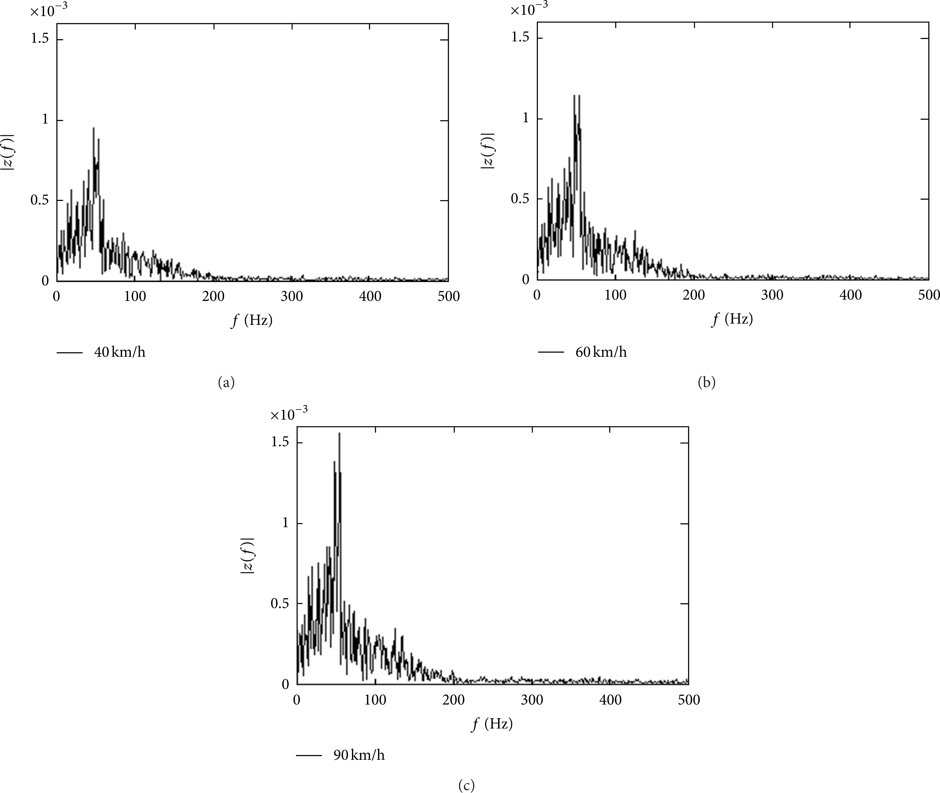
Amplitude-frequency response curves under different velocities.

Phase diagram of vehicle rear suspension travel and dynamic load is shown in Figure 5. When the load is kept in a fixed value, phase trajectory is distributed in closed domain; system in a state of quasiperiodic oscillations and suspension travel and suspension vibration dynamic load have obvious increase with the increase of speed. When speeds are 40, 60, and 90 km/h, the suspension dynamic load, respectively, accounted for 1.45%, 0.83%, and 0.67% of the static load. Summarily, there is global linear relationship between suspension travel and suspension dynamic load.

2.3.2. Simulation of Different Loads

To study the load's impact on dynamic characteristics of suspension, vehicle speed is 40 km/h and is driving on level-A road, where $G_q(n_{\mathrm{0}})=\mathrm{16}\times \mathrm{1}{\mathrm{0}}^{-\mathrm{6}}\mathrm{\hspace{0.17em}\hspace{0.17em}}$ in simulation. Vehicle load, 0 t, 5 t, and 10 t, weighs acting on rear suspension structure are 2375 kg, 6865 kg, and 10610 kg; amplitude-frequency characteristics of suspension travels are as shown in Figure 4. The spectrum analysis diagram shows that with the increase of load, amplitude of suspension dynamic load increases.

Figure 4:

Amplitude-frequency response curves under different loads.

Figure 5:

Phase diagrams under different velocities.

Phase diagram of vehicle rear suspension travel and dynamic load is as shown in Figure 6. When the speed is kept in a fixed value, phase trajectory is distributed in closed domain; system in a state of quasiperiodic oscillations and suspension travel and suspension vibration dynamic load have obvious increase with the increase of load. When the weighs acting on rear suspension are 2375 kg, 6865 kg, and 10610 kg, the suspension dynamic load, respectively, accounted for 0.71%, 0.87%, and 1.07% of the static load. Summarily, there is global linear relationship between suspension travel and suspension dynamic load.

Figure 6:

Phase diagrams under different loads.

3. Load Monitoring

3.1. Load Detecting Device

Based on above analysis about the relationship between the dynamic load and deformation of the suspension, a suspension load measurement device was developed to obtain vehicle load information. a suspension load measurement device was developed in order to attain vehicle load information. It has contained plate for joining bodywork, guyed displacement sensor, steel wire for joining sensor, overload protection structure, L-shaped plate for joining axle, and clamper for overload protection device. Whole structure of device and assembly position was showed in Figure 7. Firstly, overload protection device connects the guyed displacement sensor by the steel wire; secondly, the guyed displacement sensor which fixed on the plate for joining bodywork by fix bolt connects the side beam of chassis frame in real axle by plate for joining bodywork. Finally, overload protection structures connect the L-shaped plate which linked plate spring in real axle by cramping arrangement.

Figure 7:

Structure and installation schematic diagram of vehicle load status detection device.

The work principles of the device are as follows. When load goods to the truck and deformation of the suspension lead to relative displacement generation between the axle and chassis frame, in this process, the elastic amount of wires of the sensor also happened to be changed; the mechanical displacement can be transformed into electric signals which are measurable and proportional to linearity; voltage signals of sensor can be expressed as

$A=\left[\begin{array}{cc}{\mathrm{0}}_{\mathrm{4}\times \mathrm{4}}& I_{\mathrm{4}\times \mathrm{4}}\\ -M^{-\mathrm{1}}K& -M^{-\mathrm{1}}C\end{array}\right],\hspace{1em}\hspace{1em}B=\left[\begin{array}{c}{\mathrm{0}}_{\mathrm{4}\times \mathrm{4}}\\ M^{-\mathrm{1}}\end{array}\right],$

(16)

According to principle of measurement, as loading different weights on vehicle sensor output, voltages are different and relation between sensor output voltages and wheel vertical force need to be established to obtain load information.

3.2. Detection Platform

Vehicle load status monitoring platform was built on flat head diesel truck; it was as the test vehicle which the maximum load is 10 tons. The installation of sensors was shown in Figure 8. 400 mm of sensor wire corresponding to connecting resistance is 10 kilo-ohm and output voltage is 0∼5 v. Freescale 16-bit SCM was used as the terminal for data acquisition and preprocessing, and the program was written in CODEWARRIOR5.0; it consists of A/D conversion, signal denoising, signal transformation, and load status identification. Finally, load signal after being processed by controller was displayed by PC with programming for user interface. Platform building is shown in Figure 8.

Figure 8:

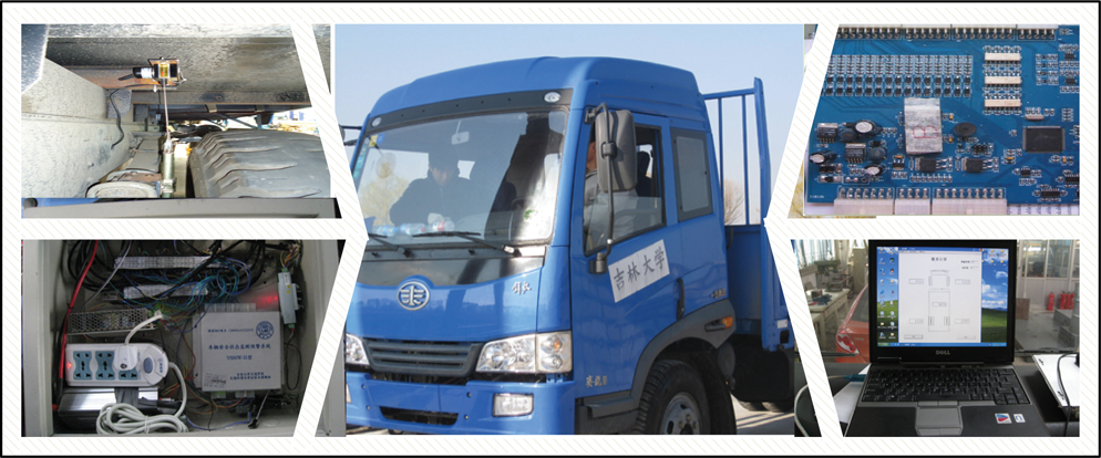
Platform of load dynamic detection.

3.3. Horizontal Center-of-Mass

Generally, the position of vehicle center-of-mass was calculated using the method of static load measurement, the body is treated as rigid body in the calculation, and the center-of-mass position is unchanged [23], however, the center-of-mass of truck is shifting when vehicle is turning and emergency is braking, bumping, and other special circumstances; accident often happens in such circumstances. Based on setting up the system of horizontal load vehicles coordinate as shown in Figure 9, position of vehicle center-of-mass was located for monitoring vehicle load status by using the method of moment balance.

Figure 9:

Coordinate system vehicle center-of-mass.

As shown in the vehicle coordinate system, the fixed position of left side of rear sensor is defined as the coordinate system origin; when vehicle loads evenly, center-of-mass is (X₀,Y₀). Length of axle is a, wheelbase is b, and balance points of torque are $P_n(x_p,b)$ , $Q_n(x_q,\mathrm{0})$ , R _n (0,y _r ), and S _n (a,y _s ). They are calculated by the moment balance principal as

$V=IR=I·kl.$

(17)

If F _mn = F _m /(F _m + F _n ), coordinates of P _n , Q _n , R _n , and S _n are $(a{F}_{21},0)$ , $(a{F}_{34},0)$ , $(0,b{F}_{14})$ , and $(0,b{F}_{23})$ . Connecting P _n and Q _n to establish equation of line, analytical expression of P _n Q _n is

$\begin{array}{c}{F}_{\mathrm{1}}{x}_p=F_{\mathrm{2}}·\left(a-x_p\right),\hspace{1em}{x}_p=\frac{a{F}_{\mathrm{2}}}{F_{\mathrm{2}}+F_{\mathrm{1}}},\hspace{1em}{P}_n\left(\frac{a{F}_{\mathrm{2}}}{F_{\mathrm{2}}+F_{\mathrm{1}}},b\right),\\ F_{\mathrm{4}}{x}_q=F_{\mathrm{3}}·\left(a-x_q\right),\hspace{1em}{x}_q=\frac{a{F}_{\mathrm{3}}}{F_{\mathrm{3}}+F_{\mathrm{4}}},\hspace{1em}{Q}_n\left(\frac{a{F}_{\mathrm{3}}}{F_{\mathrm{3}}+F_{\mathrm{4}}},\mathrm{0}\right),\\ F_{\mathrm{4}}{y}_r=F_{\mathrm{1}}·\left(b-y_r\right),\hspace{1em}\mathrm{\hspace{0.17em}\hspace{0.17em}}{y}_r=\frac{b{F}_{\mathrm{1}}}{F_{\mathrm{1}}+F_{\mathrm{4}}},\hspace{1em}{R}_n\left(\mathrm{0},\frac{b{F}_{\mathrm{1}}}{F_{\mathrm{1}}+F_{\mathrm{4}}}\right),\\ F_{\mathrm{3}}{y}_s=F_{\mathrm{2}}·\left(b-y_n\right),\hspace{1em}{y}_s=\frac{b{F}_{\mathrm{2}}}{F_{\mathrm{2}}+F_{\mathrm{3}}},\hspace{1em}{S}_n\left(a,\frac{b{F}_{\mathrm{2}}}{F_{\mathrm{2}}+F_{\mathrm{3}}}\right).\end{array}$

(18)

In the same way, analytical expression of R _n S _n is

$y_{pq}=\frac{b}{a\left(F_{\mathrm{21}}+F_{\mathrm{34}}\right)}\left(x-a{F}_{\mathrm{34}}\right).$

(19)

$(X_n,Y_n)$ is point of P _n Q _n cross R _n S _n as follows:

$y_{rs}=\frac{b}{a}\left(F_{\mathrm{23}}-F_{\mathrm{14}}\right)x+b{F}_{\mathrm{14}}.$

(20)

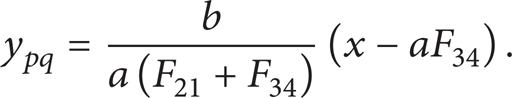
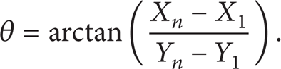
The above position of vehicle center-of-mass is given by the coordinate of intersection point. Deviation angle of center-of-mass is

$\begin{array}{c}{X}_n=\frac{a\left[F_{\mathrm{14}}\left(F_{\mathrm{21}}-F_{\mathrm{34}}\right)+F_{\mathrm{34}}\right]}{\mathrm{1}-\left(F_{\mathrm{21}}-F_{\mathrm{34}}\right)\left(F_{\mathrm{23}}-F_{\mathrm{14}}\right)},\\ Y_n=b{F}_{\mathrm{14}}+\frac{b\left(F_{\mathrm{23}}-F_{\mathrm{14}}\right)\left[F_{\mathrm{14}}\left(F_{\mathrm{21}}-F_{\mathrm{34}}\right)+F_{\mathrm{34}}\right]}{\mathrm{1}-\left(F_{\mathrm{21}}-F_{\mathrm{34}}\right)\left(F_{\mathrm{23}}-F_{\mathrm{14}}\right)}.\end{array}$

(21)

Offset of center-of-mass is

$\theta =\arctan \left(\frac{X_n-X_{\mathrm{1}}}{Y_n-Y_{\mathrm{1}}}\right).$

(22)

4. Road Test

4.1. Calibration Test

The formulas describing relation between load information and sensor voltage are deduced by static calibration test; test was carried on in FAW truck and testing ground as shown in Figure 10; maximum loading quantity of truck is 14 tons; Vehicle was no-loading in the first set of test and added 0.5 tons weight every time before the next set of test, the maximum loading is 14 tons; meanwhile weight of wheel vertical load was measured using CAS axle load meter; four groups of sensor output voltage value were collected from terminal; 28 sets of data were recorded. The relation of load quadratic fits as shown in Figure 11; calibration formula is obtained as

$L=\sqrt{{\left(X_n-X_{\mathrm{1}}\right)}^{\mathrm{2}}+{\left(Y_n-Y_{\mathrm{1}}\right)}^{\mathrm{2}}}.$

(23)

$\begin{array}{c}{M}_{Lf}=\mathrm{0.0028}{U}_{Lf}^{\mathrm{2}}-\mathrm{10.7253}{U}_{Lf}+\mathrm{11768},\\ M_{Rf}=\mathrm{0.0032}{U}_{Rf}^{\mathrm{2}}-\mathrm{11.7253}{U}_{Rf}+\mathrm{12387},\\ M_{Lr}=\mathrm{0.0030}{U}_{Lr}^{\mathrm{2}}-\mathrm{12.0749}{U}_{Rr}+\mathrm{12899},\\ M_{Lf}=\mathrm{0.0049}{U}_{Lf}^{\mathrm{2}}-\mathrm{20.9151}{U}_{Rf}+\mathrm{23169},\end{array}$

(24)

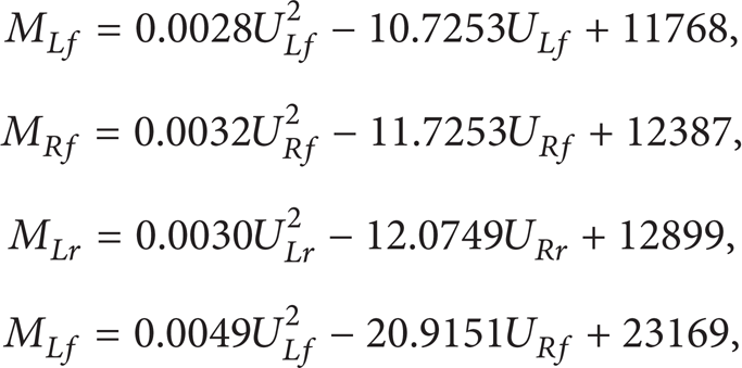
where U is sensor output voltage and M is tire vertical loads; tire truck loads were calculated by the previous formula.

Figure 10:

Fitting test.

Figure 11:

Quadratic fitting.

4.2. Measuring Precision Test

The accuracy of the measurement of wheel load was tested, respectively, in different speeds and different loaded weights; experimental parameters are as shown in Table 2.

Table 2:

Test parameters.

Parameter name	Parameter value
Testing road	Level-A, body twist lane
Sampling frequency	30 Hz
Velocity	40 km/h, 60 km/h, 90 km/h
Load	0 t, 2.5 t, 5 t, 7.5 t, 10 t

Maximum loading quantity of test is 14 tons; vehicles was no-load in the first set of test and add 2.5 tons weight to the truck before the next set of test, maximum loading in the test is 10 tons; meanwhile CAS static axle load meter is used to measure the total mass of vehicle. Drove on Level-A road, respectively, in the speed of 40 km/h, 60 km/h, and 90 km/h, load information was real-time collected and displayed on vehicle computer and data was stored in memory in EXCEL format.

Mean of 15 sets of load data were solved under different loading conditions and the speed. Total mass of vehicle is the sum of four wheel loads; results are obtained as shown in Table 3; the deviation of measured value is shown in Figure 12; the test results show that measurement error is less than 5% in different speeds and load conditions; results meet the requirements of the measurement system. Monitoring results can be used to determine whether the vehicle was overloaded.

Table 3:

Vehicle loading measurement result.

Loading quality	Weigh (ALM)	40 km/h	60 km/h	90 km/h
0 t	4920	4839.8	4826.4	4828.8
2.5 t	7205	6972.7	6900.8	6851.9
5.0 t	9665	9387.5	9409.0	9416.9
7.5 t	12080	11584	11489	11539
10 t	14570	14771	14484	14525

Figure 12:

Vehicle loading deviation.

4.3. Center-of-Mass Detecting Test

To test the feasibility of method for center-of-mass estimation, experiment of center-of-mass position detection was tested on the body twist lane; vehicle loading quantity is 5 tons. Figure 13 shows the live and description of body twist lane.

Figure 13:

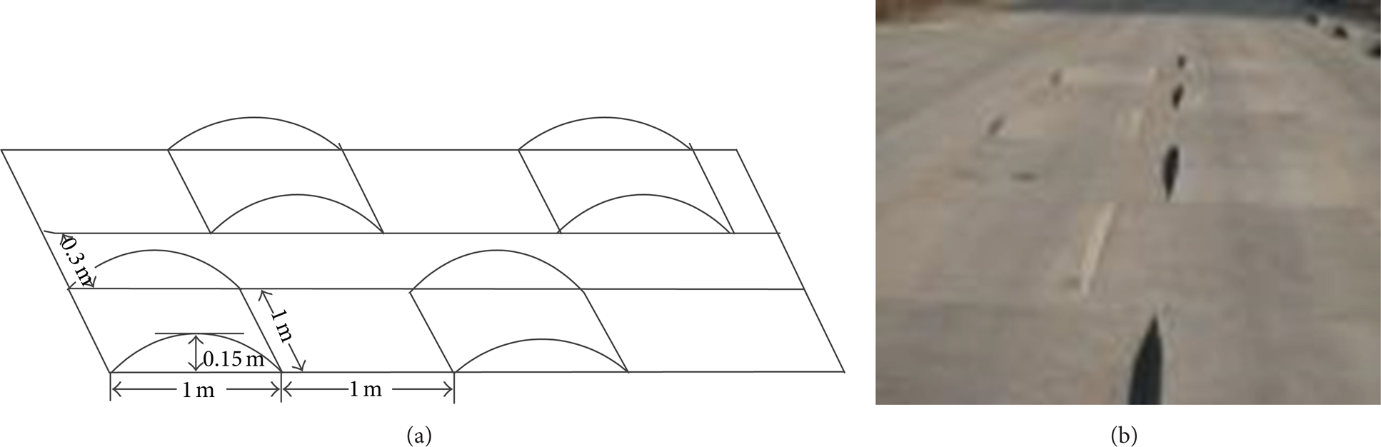
Waveform distortion road.

Drive testing vehicle on the body twist lane and left and right sides of the wheel get across distortion pavement which alternate with height of 0.15 m and length of 1 m. Figure 14(a) shows time 3D trajectory of vehicle horizontal center-of-mass; it was calculated by (21). Figure 14(b) was the phase diagram of center-of-mass. Figures 14(c) and 14(d) were the trajectory of center-of-mass coordinates projection on the x-axis and y-axis.

Figure 14:

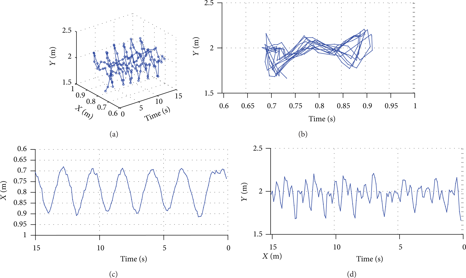
Center-of-mass track.

Vehicle dived on body twist lane ebb and flows in cycles as shown in Figure 15(a); the phase diagram of center-of-mass was shown in Figure 15(b). Figures 15(c) and 15(d) were the trajectory of center-of-mass coordinates projection on the x-axis, y-axis. When moving vehicles meet the slope of body twist lane, the left-front wheel was raised and the center-of-mass was moving to the right rear and then moves to left-front with driving downhill; the right-front wheel of the moving vehicles was raised when meeting the slope of distortion road; center-of-mass was moving to the left rear and then moves to right-front with driving downhill; vehicles running on body twist lane go through several cycles rise and fall at low speed; the change of center-of-mass position repeats the above trajectory as shown in Figure 15(a).

Figure 15:

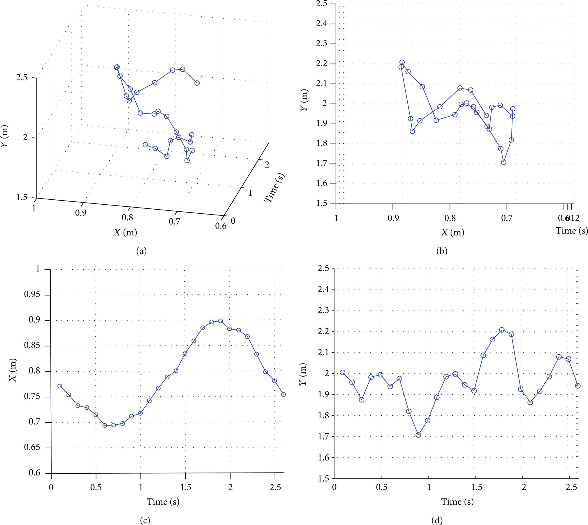
Single cycling track of center-of-mass.

To summarize the above:

1. when vehicle is driving on body twist lane, the 3D track of center-of-mass was periodic cycle;

2. trajectory of center-of-mass coordinates projecting on the x- and y-axes (Figures 15(c) and 15(d)) showed that change of centre-of-mass position is periodic with undulating slopes of body twist lane; it was proved that the method is feasible in the aspects of applicable properties;

3. the status of load distribution and mass shifting was monitored by tracking the horizontal position of center-of-mass; it can also judge situation that goods are shifting and sliding off in transit.

5. Conclusions

(1) Half of vibration model of nonindependent suspension vehicle was established and simulation method of road roughness was studied in this project. Model was simulated in MATLAB/Simulink and suspension characteristics were analyzed under different working conditions; conclusion proved that suspension travel and suspension dynamic load were interrelated in global linear relationship.

(2) Based on analyzing suspension characteristics, detection device for vehicle load with overload protection structures was developed and values of sensor voltage were calibrated by tire vertical load in static rowing test.

(3) Monitoring platform for vehicle load status was built on the truck; the monitoring method of vehicle load status was proposed, but accuracy of center-of-mass positioning still needs to be tested and verified in next step; threshold of vehicle safety determination needs to be validated in further research.

(4) Road test shows that system measurement error is less than 5% under different working conditions, and horizontal center-of-mass of vehicle was positioned correctly. Research provides technical support for the real-time monitoring and warning of vehicles risk status in transit.