Sage Journals: Discover world-class research

Abstract

This study focuses on cutting force predictions with the tool-workpiece inclination angle in bull-nose milling based on the semimechanistic force model. By analyzing kinematics and mechanics of the bull-nose end mills during cutting, force expressions including lead angle are stated and the model is exerted on each discrete element as oblique cutting with coordinate transformation and numerical integration to obtain the dynamic cutting force components. An improved identification method considering speed variations along the tool axis is applied to calibrate coefficients. Coefficients are regarded as the function of each elemental elevation. Then, a geometry-based method to acquire cutter workpiece engagement (CWE) is proposed. Also acquisition of accurate start and exit angles on each slice is deliberated elaborately for cutters with lead or tilt angle in milling processes. Thereby, to verify the validity of the force prediction model and start-exit angle acquisition method, experiments with variable lead angles are conducted under different axial immersions. The results reveal that the presented model and approaches can predict cutting forces with high accuracy. Finally, the cutting force components under different cutter postures and conditions are analyzed to provide instructions for parameter selections.

1. Introduction

Machining parts with sculptured surface are extensively used in automotive, mold, and aerospace industries such as turbine blades, impellers, and mold cavities. To obtain better tool accessibility and desired surfaces, ball-end and bull-nose mills are adopted with inclination angles between tool and workpiece in 4-axis and 5-axis CNC machining frequently. During manufacturing processes, cutting forces have great effects on cutting heat, tool wear, tool life span, deflections, and the quality of machined surface. And the complexity of cutter/part structures and cutting condition makes it difficult to select optimal machining parameters and guarantee high machining quality and efficiency. Therefore, establishing appropriate cutting force prediction model can be a driving impulse to analyze the cutting process and solve the problem of metal machining problems. However, many factors may influence the machining process, such as workpiece material, tool geometrical variables, and cutting conditions incorporating cutting depth and tool orientation. To maintain good cutting performance and avoid interference collision between cutter and workpiece, certain lead or tilt angles with respect to the tool axis is defined. Inclination angle affects cutting forces significantly and the cutting force further affects the machining efficiency and surface quality. However, most of the early works about cutting force predictions with lead angle focus on ball-end mill, and few are concentrated on bull-nose mill and its parameter acquisitions such as start/exit angle.

Up to now, numerous works have been performed on cutting force modeling, and mainly three types are involved: analytical modeling [1 –3], mechanical modeling [4 –6] and finite element modeling [7]. Li et al. [8 –10] had developed a theoretical cutting force model of oblique cutting for helical end mill by incorporating workpiece properties, tool geometry, and cutting conditions. The theoretical modeling explains the cutting mechanism and material constitutive flow principle; however, it makes some simplifications and complicates analytical calculations with massive experiments, low accuracy, and narrow application scope.

In the mechanistic method, cutting forces are assumed to be proportional to uncut chip thickness or cutter swept volume. This modeling comprises two types: the first is the combined mechanism model integrating the effects of shearing on rake face and ploughing at cutting edges by one single coefficient and the second one is dual mechanism force model separating the two different effects. Engin and Altintas studied the geometry of a generalized mathematical model wrapped by helical flutes around a parametric envelope [11], and cutting forces were then predicted by integrating the process along each cutting edge. Gradisek and other researchers developed expressions for semimechanistic identification of shearing and edge force coefficients including helix angle in the evaluation of average edge force [12]. Besides, a simplified and efficient calibration method to estimate the force coefficients for ball-end milling was proposed [13]. And only a single half-slot cut was needed to calibrate empirical force coefficients which was just valid for ball-end mills with two cutting edges. Also a new method to model and predict the instantaneous cutting forces in 5-axis milling [14] reduced prediction errors effectively based on the kinematic analysis. It is proved that the method had the ability to be used in simulations and optimizations of multiaxis machining. The reality shows that changing cutting speeds along cutting edges affects forces significantly, but the mentioned studies did not cover these influences during force prediction process.

Although approaches to model the cutting forces have been investigated in-depth, only limited literature focused on taking the effects of lead or tilt angle into mechanistic cutting force modeling and getting accurate engagement area participated in the cutting process. For ball-end milling, effects of lead angle on cutting forces were predicted through simulations using the process model drawn by Ozturk and Budak [15]. While Ozturk and Tunc presented the detailed analysis of lead and tilt angle's effects on cutting forces, torque, form errors and stability [16]. Also researches that dealt with the effects of tool-surface inclination on ball end mill cutting forces were conducted by using thermomechanical modeling of oblique cutting [17, 18]. Based on this model, Fontaine et al. launched several experiments with straight tool paths and various tool-surface inclinations on a 3-axis machine. By doing this, it identified the optimized inclination angle as well as the influences of cutting condition, radial run-out, ploughing, and cutting stability on ball-end mill [18]. Later, they studied the maximum values of three cutting force components considering inclination angle to determine the favorable tool orientation and limit the deflection for the certain cutter [19]. Attention was also given to the analysis of the undeformed chip geometry and cutter-workpiece contact area using Z-map data for ball end mill by Kim et al. [20]. Meanwhile, Cao et al. proposed a new experimental method to identify the force coefficients including the inclination angle in finish milling for ball-end mill, and it was superior to the slot experimental method [21].

It is interesting to estimate that studies on the cutting force predictions with lead angle mainly concentrate on ball-end mill, and little information on bull-nose mill is proposed. Therefore, to get accurate cutting forces and tool-workpiece engagement area for bull-nose end mills, this paper presents a semimechanistic model and a geometry-based approach to calculate cutting forces as well as contact area, respectively. Firstly, it calibrates cutting force coefficients by adopting an improved method through force model proposed by Altintas. The method recalculates cutting forces in each discretized layer during identification processes due to various cutting speeds along tool axis. Then it develops the force calculation derivations by taking the lead angle influences into account. The transformation matrix is changed from the early expressions. One contribution lies in that the lead angle and different speed influences are involved in the process of discretising along the tool axis, and a geometry-based method to get start-exit angle is proposed. The coefficient identification method and contact area acquisition method can be extended to other conditions such as tilt angle and different tool types with high accuracy. At last, the semimechanistic method is applied to predict the cutting force. And validation tests are conducted under different cutter postures and cutting conditions. The comparison between predicted and measured values demonstrates the applicability of the model and approach of cutting forces and coefficients. Finally, the trend of cutting force components under different cutting conditions is analyzed in tool-workpiece inclination milling for further cutting parameter selections and optimization.

2. Geometry of Bull-Nose End Mills

The basic structure of a bull-nose end mill can be subdivided into three sections: tool shank, cylindrical surface, and loop surface. Bull-nose end mill is an amelioration of sharp-edged flat end tool that connects the bottom cutting edge with one side to form a loop surface, while the participated cutting surface is not the whole loop but only a characteristic curve on it that functions as a cutting edge on flat end mill. The multiple helical cutting edges on both its periphery and its tip require seven parameters D,R,R_r,R_z,α,β, and h, respectively, to distinguish general helical end milling cutters such as cylindrical mill, bull-nose mill, and taper mill. The detailed parameters of a bull-nose end mill are with D,R,R_r,R_z,h≠0, α = β = 0 depicted in Figure 1. Three zones define the cutter envelope where parameters such as immersion angle κ(z), radial distance R, elemental elevation z, arc radius r(z), and helical angle are accounted diversely.

Figure 1:

Bull-nose end mill geometry.

Figure 2 shows a solid model of a generalized tool with local cutting force coordinate X′Y′Z′ and the machining coordinate XYZ which has the origin located in the point where the tool axis intersects with its face plane. The positive directions of axes X and Y are aligned with feed direction and normal direction of machined surface, and the Z direction designates the tool axis, respectively, following the right-hand convection. Analysis of tool geometry, chip load, and cutting force components makes forces calculation acting on each cutting edge available. Accordingly, three components including the tangential, axial, and radial can be gained by dividing the tool axis into a finite number of elements, and related parameters and conversion along cutting edges are supposed to be defined. Cutting force components on each element are illustrated with dF_a, dF_r, and dF_t at cutting point P with the elevation z. The axial immersion angle of point P is the angle between Z-axis and normal of helical cutting edge. Figure 2 describes related parameter definitions from the perspective of front view and cross-section top view.

Figure 2:

Geometric model.

The position of point P on the cutting edge is defined by axial distance z, radial distance r(z), axial immersion angle κ(z), radial lag angle ψ(z), and so on. Radial immersion angle ϕ_i,j(φ) referring to the jth axial disk element of the ith flute at elevation z measured clockwise can be expressed as

ϕ_{i, j} (φ) = φ + \frac{2 (i - 1)}{N} - ψ (z),

(1)

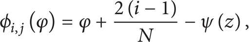
where φ denotes the immersion angle of the reference edge j = 1 at tool tip, and it is called spindle rotation angle. While ϕ_i,j(φ) is the angular position of the jth layer on the ith flute at the current rotation angle φ with N_t teeth evenly spaced around the tool axis. ψ(z) is the angle between line r(z) and the line where cutting edge is tangent to the tip of cutter. The two different zones in bull-nose tool are expressed.

Arc zone MN(0<z ≤ R): the radial offset at elevation z together with the axial immersion angle can be deduced as

r (z) = \frac{D}{2} - R + \sqrt{R^{2} - {(R - z)}^{2}} κ (z) = arccos \frac{R - z}{R} .

(2)

In the MN zone, due to changing radial radius along the tool axis, helical angle varies along the flute with constant lead. This design is preferred by cutter grinders to save material during regrinding operation, while, in (3), i₀ is the invariable helix angle in cylinder part, and i(z) is the changing angle in the current zone

i (z) = ta n^{- 1} (\frac{(r (z) - R_{r}) \tan i_{0}}{R}) .

(3)

The bull-nose end mill model involved in this paper has a full quarter circle which is tangent to the cylindrical zone and the bottom part of the cutter. Therefore, lag angle can be written as

ψ (z) = \frac{z}{R} \tan i_{0} .

(4)

Cylindrical zone NS (R<z ≤ h): r(z) and κ(z) are constant as

r (z) = \frac{D}{2} κ (z) = \frac{π}{2} .

(5)

This area can be regarded as the cylindrical end mills, and the expression is easy to conclude

i (z) = i_{0} ψ (z) = \frac{2 z \tan i_{0}}{D} .

(6)

Since the instantaneous uncut chip thickness varies according to the variation of the cutting edge position, it can be obtained through

h_{i, j} (z) = f_{t} \sin ϕ_{i, j} (z) \sin κ (z),

(7)

where $f_{t} (f_{t} = v_{f} τ)$ refers to the feed per tooth of the jth tooth, $τ = 60 / (N * Ω)$ is the tooth passing period, and v_f is the feed speed. And Ω is the spindle speed in revolutions per minute (rpm). To denote the location of elemental cutting edge, $\overset{⃑}{r}$ is defined as

\overset{⃑}{r} = r (z) (\overset{⃑}{i} \sin ϕ_{i, j} + \overset{⃑}{j} \cos ϕ_{i, j}) + \overset{⃑}{k} z (ϕ_{i, j}) .

(8)

3. Mechanistic Cutting Force Model

Based on the tool geometry, a semimechanistic cutting force model is established to determine cutting forces by analysing whether its cutting edge is involved in milling process. Along the tool axis, its cutting edge is discretised into slices to account for the helical angle effect on the cutting forces and the cutting actions of each element function as an oblique cutting process. Therefore, the whole cutting force exerted on the workpiece can be obtained through integrating all the discs along cutting edges. In the process of calculation, first judge the number of elements that are engaged in cutting; then adopt start/exit angle method to determine whether the current cutting disc is involved. Because of the loop surface in bull-nose end mill and inclination angle between the cutter axis and workpiece surface, start and exit angles in different layers vary either.

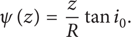
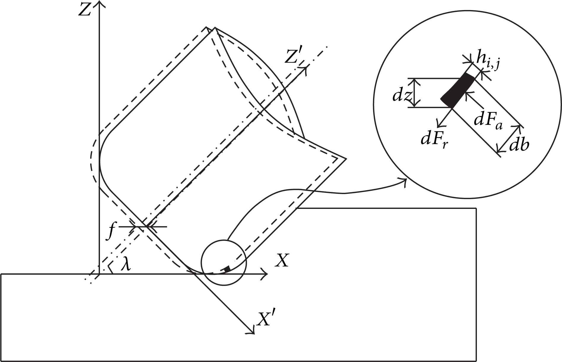
Figure 3 shows the explicit bull-nose end mill geometry with lead angle in cutting process. The X′Y′Z′ is a coordinate system with the positive direction X′ deviated from the absolute coordinate X with the angle λ, and Z′ axis is perpendicular to the rotation plane. Referring to this coordinate system, cutting edge segment is viewed as a single-point cutting tool; thus cutting force components are produced in this segment in the tangential, radial, and axial direction, respectively. The force components acting on the elevation dz are shown as

\begin{matrix} d F_{t, j} (ϕ, z^{'}) = K_{t c} h_{i, j} (z^{'}) d b + K_{t e} d s, \\ d F_{r, j} (ϕ, z^{'}) = K_{r c} h_{i, j} (z^{'}) d b + K_{r e} d s, \\ d F_{a, j} (ϕ, z^{'}) = K_{a c} h_{i, j} (z^{'}) d b + K_{a e} d s, \end{matrix}

(9)

where dF_t,j(ϕ, z′), dF_r,j(ϕ, z′), and dF_a,j(ϕ, z′) refer to the tangential, radial, and axial instantaneous cutting forces when the spindle angle reaches ϕ with the jth edge at elevation z. The K_tc,K_rc,K_ac and K_te,K_re,K_ae are the corresponding orthogonal cutting force coefficients, and K_sc,K_se (s = t,r,a) denote effects of shearing on the rake face and the rubbing at the cutting edge, respectively. Then db and ds are the instantaneous uncut chip width and the contact distance of cutter edge element. Thus, db (db = dz′/sinκ(z′)) is the projected length of an infinitesimal cutting flute in the direction of the cutting velocity. And ds refers to the infinitesimal length of cutting edge segment which can be written as $d s (z^{'}) = d z^{'} \sqrt{{(r (z^{'}) ψ^{'} (z^{'}))}^{2} + {(r^{'} (z^{'}))}^{2} + 1}$ . The superscripts followed after r and ψ denote the derivative with regard to z′. Due to the lead angle in cutting conditions, λ is introduced to reflect the angle between X-axis in the machining coordinate system and Z′-axis in the tool coordinate system. The expression of instantaneous uncut chip thickness changes into

h_{i, j} (z^{'}) = f_{t} \sin ϕ_{i, j} (z^{'}) \sin κ (z^{'}) \sin λ .

(10)

Figure 3:

Geometric model with lead angle.

By substituting (10) into (9), instantaneous cutting forces are expressed as

\begin{matrix} d F_{t, j} (ϕ, z^{'}) = K_{t c} h_{i, j} (z^{'}) f_{t} \sin ϕ_{i, j} (z^{'}) \sin λ d z^{'} + K_{t e} d s, \\ d F_{r, j} (ϕ, z^{'}) = K_{r c} h_{i, j} (z^{'}) f_{t} \sin ϕ_{i, j} (z^{'}) \sin λ d z^{'} + K_{r e} d s, \\ d F_{a, j} (ϕ, z^{'}) = K_{a c} h_{i, j} (z^{'}) f_{t} \sin ϕ_{i, j} (z^{'}) \sin λ d z^{'} + K_{a e} d s . \end{matrix}

(11)

Through coordinate transformation, the cutting force in the X′Y′Z′ coordinate system can be obtained:

[\begin{bmatrix} d F_{x^{'}, j} (ϕ, z^{'}) \\ d F_{y^{'}, j} (ϕ, z^{'}) \\ d F_{z^{'}, j} (ϕ, z^{'}) \end{bmatrix}] = [\begin{bmatrix} - \cos ϕ_{i, j} & - \sin κ \sin ϕ_{i, j} & - \cos κ \sin ϕ_{i, j} \\ \sin ϕ_{i, j} & - \sin κ \cos ϕ_{i, j} & - \cos κ \cos ϕ_{i, j} \\ 0 & \cos κ & - \sin κ \end{bmatrix}] \times [\begin{bmatrix} d F_{t, j} (ϕ, z^{'}) \\ d F_{r, j} (ϕ, z^{'}) \\ d F_{a, j} (ϕ, z^{'}) \end{bmatrix}] .

(12)

Cutting forces at any rotational moment acting on the jth cutting edge can be get by integrating (12) along the axial cutting depth

[\begin{bmatrix} F_{x^{'}, j} (ϕ, z^{'}) \\ F_{y^{'}, j} (ϕ, z^{'}) \\ F_{z^{'}, j} (ϕ, z^{'}) \end{bmatrix}] = [\begin{bmatrix} \int_{0}^{z^{'}} d F_{x^{'}, j} (ϕ, z^{'}) \\ \int_{0}^{z^{'}} d F_{y^{'}, j} (ϕ, z^{'}) \\ \int_{0}^{z^{'}} d F_{z^{'}, j} (ϕ, z^{'}) \end{bmatrix}] .

(13)

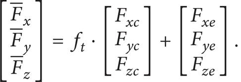
The total forces in the machining coordinate system are illustrated, since the measured cutting force is under this coordinate either. They contain lead angle effects into transformation matrix varying from the traditional formula; therefore, the similar process can also be used in the derivation when accounting for tilt angle influences. In addition, only when cutter teeth are in the cutting process, they contribute to the forces and should be judged before summation. If sweeping angle (ϕ_s = ϕ_ex – ϕ_st) is larger than pitch angle, one more cutter tooth participates in the cutting process which should be paid attention to. And the cutting depth of different teeth varies as well as each force. So the final expression can be written as

[\begin{bmatrix} F_{x} (ϕ, z) \\ F_{y} (ϕ, z) \\ F_{z} (ϕ, z) \end{bmatrix}] = T_{1} [\begin{bmatrix} \sum_{j = 1}^{N} F_{x^{'}} (ϕ, z^{'}) \\ \sum_{j = 1}^{N} F_{y^{'}} (ϕ, z^{'}) \\ \sum_{j = 1}^{N} F_{z^{'}} (ϕ, z^{'}) \end{bmatrix}] = T_{1} T_{2} [\begin{bmatrix} \sum_{j = 1}^{N} \int_{0}^{z^{'}} d F_{t, j} (ϕ, z^{'}) \\ \sum_{j = 1}^{N} \int_{0}^{z^{'}} d F_{r, j} (ϕ, z^{'}) \\ \sum_{j = 1}^{N} \int_{0}^{z^{'}} d F_{a, j} (ϕ, z^{'}) \end{bmatrix}]

(14)

with

\begin{matrix} T_{1} = [\begin{bmatrix} \sin λ & 0 & \cos λ \\ 0 & 1 & 0 \\ - \cos λ & 0 & \sin λ \end{bmatrix}], \\ T_{2} = [\begin{bmatrix} - \cos ϕ_{i, j} & - \sin κ \sin ϕ_{i, j} & - \cos κ \sin ϕ_{i, j} \\ \sin ϕ_{i, j} & - \sin κ \cos ϕ_{i, j} & - \cos κ \cos ϕ_{i, j} \\ 0 & \cos κ & - \sin κ \end{bmatrix}] . \end{matrix}

(15)

4. Tool and Workpiece Engagement Area Acquisition

The acquisition of tool-workpiece engagement area is the basis for calculating start and exit angles and also the prerequisite condition to obtain cutting forces. Therefore, by handling bull-nose end mill under various lead angles as finite tiny slices along cutter orientation, the engagement area is then calculated by the following algorithm. The instance about slot milling is given in certain lead angles to determine engagement area, further to get start-exit angles utilised in the calculations of bull-nose end mill. Although the examples are all about bull-nose end mill, the area acquisition method has wider application which can also be employed to other helical mills.

Engagement area locates between rotary surface rotated by cutter edges and workpiece. Through the feed-rate direction, this engagement area reflects the instantaneous cutting state of bull-nose end mill with the workpiece. Figure 4 shows an example of engagement area in different directions: vertical to feed direction and parallel to negative feed direction.

Figure 4:

Engagement area in different directions ((a) vertical to feed direction, (b) parallel to negative feed direction).

In order to obtain the area, machining surface is defined which is identified by whether the lead angle is zero or not shown below.

(1) λ = 0. The normal vector of machining surface is parallel to the cutter orientation; meanwhile the surface is overlapped with cutter bottom surface. By offsetting the machining surface equal to machining residual value along the direction of machining surface normal vector, blank surface can be gained as shown in Figure 5(a).

Figure 5:

Cutter posture without lead angle ((a) λ = 0) and with lead angle ((b) λ≠0).

(2) λ≠0. The normal vector of machining surface is inclined λ from the cutter orientation. To get it, first define a random surface below the cutter solid which is parallel to machining one, and then account for the nearest point to the random, namely, the tangent point of machining surface and cutter solid. Then offset the machining surface through its normal vector with the residual distance, and that is the blank surface illustrated in Figure 5(b).

According to definitions, the slice-based method is presented to acquire the area. Firstly, insert finite surface slices between machining and blank surfaces which intersects with cutter solid until reaching the height of blank surface; secondly, through the negative feed direction, their intersection lines as well as the contour line of cutter bottom converge into a number of reference points; thirdly, a spline curve is fitted by utilising the data of reference points and tangent point obtained above, together with the intersection line between cutter solid and blank surface; then engagement area boundary can be fixed. In the process of solving the engagement area, the precision can be guaranteed through the plane quantity. As shown in Figures 6 and 7, the chart gives an explanation of the process, while 3D display expresses the defined conception and relationship of the relevant factors.

Figure 6:

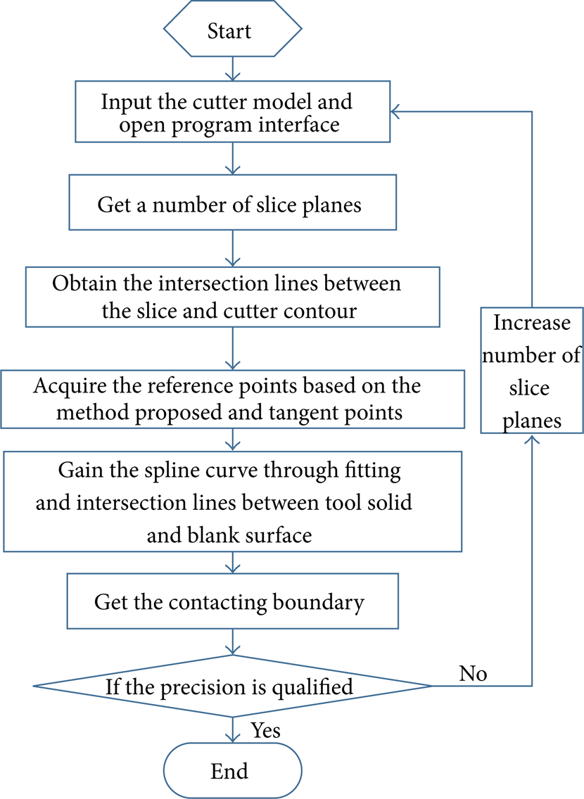
The process of calculating contacting boundary.

Figure 7:

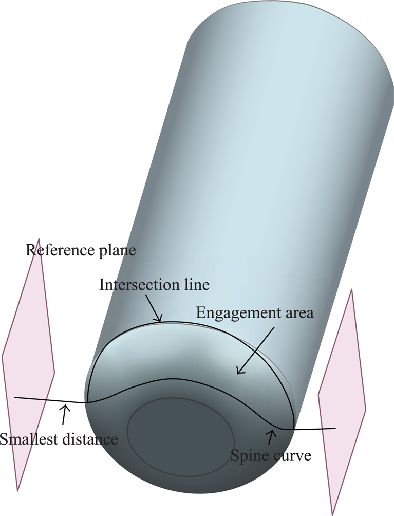
Reference schematic diagram.

Accurately calculating and choosing the inclination angle between the tool axis and workpiece surface can not only eliminate collision and improve cutting condition but also decrease the vertical cutting forces. Based on the proposed method, several illustrations of engagement area are given on the condition that the axial depth is 1 mm and six inclinations angles are 5°, 10°, 12°, 15°, 18°, and 20°, respectively. And tool parameters are illustrated in experimental setup part. From Figure 8, it can be seen that different cutter gestures have varying contact boundaries that affect contact zones.

Figure 8:

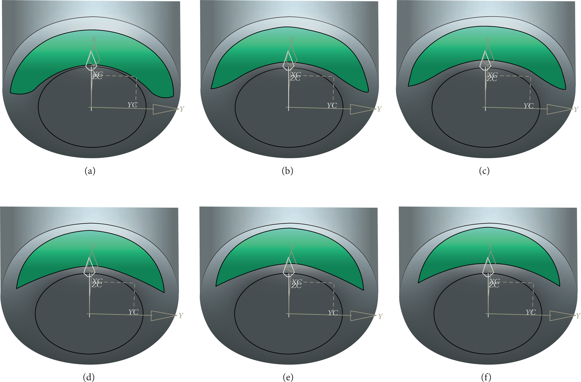
Tool and workpiece engagement area in different inclination angles ((a) angle 5°, (b) angle 10°, (c) angle 12°, (d) angle 15°, (e) angle 18°, and (f) angle 20°).

The examples are slot milling process, and the same method can also be extended to other milling situations such as side milling with free-form surfaces. Nevertheless, some changes about engagement boundary substitution make the solution possible. As referred above, the input factor into 3D software should be accompanied with the shape of surface to be machined; thus several modifications of the second development program based on commercial software are required either. Instances of engagement region acquisition in ball-end milling with lead and tilt angles together with free-form workpiece are illustrated in Figure 9.

Figure 9:

Tool and workpiece engagement area under different lead and tilt angles.

5. Identification of Specific Force Coefficients

The accurate evaluation of coefficients of a cutting force model is essential to the reliability of the predicted forces. Note that, for bull-nose mill, the cutting conditions vary dramatically along the cutting edge as the cutter rotates. Thus, the instantaneous measured cutting forces at each cutting instant are applied to identify the coefficients. Since the average cutting forces obtained through experiments and that got from the derivation of cutting force calculation equations are equal, this conception can be used to render the cutting force coefficients. Because the total cutting material in one tooth period cutting process has no relationship with the helical angle, the average cutting forces are independent of helical angle. So the average forces are shown:

{\overset{⃑}{F}}_{*} = \frac{1}{ϕ_{p}} \int_{ϕ_{s t}}^{ϕ_{e x}} F_{*} (ϕ) d ϕ .

(16)

In (16), milling is an intermittent cutting process in which ϕ_ex, ϕ_st designate the jth tooth that enters and exits the cut, respectively, in Figure 9. For up-milling operations, ϕ_ex = 0 and if D refers to the tool diameter and d_r represents radial immersion depth then $ϕ_{s t} = arccos ((D - 2 d_{r}) / D)$ . However, it's difficult to determine ϕ_ex and ϕ_st in the experiments with inclination angles.

Two methods (geometry-based method and analytical method) can be applied to get start and exit angles in the force prediction process. While, for tool/workpiece with complicated surfaces, the second one is sophisticated in its boundaries and formulations, it brings barrier to precisely depict the curve. Meanwhile, the calculation is determined by dividing the cutting edge into a finite number of discs; thus intersection solution and accurate computing may be inconvenient. Nevertheless, analytical geometry-based method does not need accurate expressions of intersection curves with the aid of the 3D formative software. The concrete approach is presented as Figure 10 working as the core algorithm embedded in a module which can be achieved automatically. In the current presentation, to simplify and decrease the calculation time, 9 discs of the same thickness are chosen to divide engagement area and then export the contact angles shown in Table 1.

Table 1:

Start and exit angles (unit: rad) in different inclination angles (unit: °).

Angle\discs	1	2	3	4	5	6	7	8	9

5°
ϕ_st	0.238	0.159	0.122	0.099	0.083	0.070	0.354	0.699	1.200
ϕ_ex	2.903	2.983	3.019	3.042	3.059	3.072	2.787	2.443	1.941
10°
ϕ_st	0.457	0.298	0.226	0.181	0.330	0.513	0.711	0.946	1.314
ϕ_ex	2.685	2.844	2.916	2.961	2.812	2.629	2.431	2.196	1.828
15°
ϕ_st	0.462	0.347	0.356	0.473	0.594	0.723	0.867	1.040	1.295
ϕ_ex	2.679	2.794	2.786	2.668	2.547	2.418	2.275	2.102	1.846

Figure 10:

The flow chart to calculate the start-exit angle.

According to derivation, average cutting force of each cutter tooth in one cutting period can be expressed. Parameters are calculated through cutting force identification experiments. Each meaning of F_lm (l = x,y,z and m = c,e) is determined by the subscript; for instance, and F_x,c is the function of cutting force coefficients in x-axis representative of chip shearing

[\begin{bmatrix} {\bar{F}}_{x} \\ {\bar{F}}_{y} \\ {\bar{F}}_{z} \end{bmatrix}] = f_{t} \cdot [\begin{bmatrix} F_{x c} \\ F_{y c} \\ F_{z c} \end{bmatrix}] + [\begin{bmatrix} F_{x e} \\ F_{y e} \\ F_{z e} \end{bmatrix}] .

(17)

In order to simplify cutting force coefficients identification process, the identification adopts slot milling experiments in which ϕ_ex = π, ϕ_st = 0. The experiments are conducted under a series of different feed rates with various cutting forces. With measured data, coefficients can be handled through the curve fitting method. Cutting speed variations along the tool axis affect coefficients in different layers significantly. According to the procedure, the total forces are regarded as the sum of the forces on each tooth segment at every slice, so an individual disc has its own cutting force coefficients which are independent of its adjacent discs.

A case in point is that the measured cutting force cannot be used directly, whereas they should be recalculated by the current layer and its previous adjacent one. For instance, the functional value adopted by the above model has the expressions in (18). However, in the formulations, {F₁,F₂⋯F_n} represents the cutting force corresponding to the {1, 2⋯n} th element along cutter edge

\begin{matrix} F_{x_{1}} = F_{1} \\ F_{x_{2}} - F_{x_{1}} = F_{2} \\ F_{x_{3}} - F_{x_{2}} = F_{3} \\ ⋮ \\ F_{x_{n}} - F_{x_{n - 1}} = F_{n} . \end{matrix}

(18)

The experiments about coefficient identification were conducted at a set of certain cutting depths, from which six different coefficients can be obtained by cubic polynomial fitting. Each coefficient in certain disc works as the input factor of predicted cutting force with lead angles by taking speeds influences into discrete layer. Characterized by tool's periphery, various speeds along cutting orientation affect coefficients acquisition significantly and, by taking these impacts into account, it makes coefficients calculation more accurate.

6. Experimental Validation and Discussion

Two types of cutting tests are performed: one is for coefficients identification and the other is for verification of cutting forces with inclination angle. In the first setup, a total of 30 cutting tests with Al-7075 are at a series of axial cutting depths and variable feed rates. The cutting tool is 10 mm in diameter, 4 fluted bull-nose mill with constant lead distance in arc zone and 45^° helix angle in cylindrical zone which is an anticlockwise rotating tool shown in Table 2. The cutting force coefficients are calculated from slot milling by using the method. Moreover, the identification operation is with the cutting depth of 0.4, 0.8, 1.0, 1.2, 1.4, 1.6 mm, feed rates are 0.02, 0.04, 0.06, 0.08, 0.10 mm/tooth, and the spindle speed is 3000 rpm. The machining test is conducted with coolant in a 3-axis milling machine, and, as required by the inclination angle, a special fixture is needed to provide accurate angle value. Lastly, the DEWESoft6.5 software is applied to collect the sample data for later disposal.

Table 2:

Tool parameters.

Tool diameter (mm)	Arc radius (mm)	Cutting edge length (mm)	Tool holder length (mm)	Teeth number	Helix angle (°) in cylindrical part

10	2	20	75	4	45

It is shown that K_tc, K_rc, K_ac have the larger changing ranges whereas the other coefficients fluctuated slightly in Figure 11. The shearing coefficients experience large fluctuations especially in lower cutting depth characterized by side effect, while ploughing coefficients have smaller changing range and value. By substituting coefficients model into cutting force model, forces in different conditions can be predicted.

Figure 11:

Cutting force coefficients identification.

Figure 12 shows the flow chart for estimating cutting force coefficients from down milling at various feed rates and then attaining cutting forces with coefficients determined by three-order polynomial fitting procedure. Since the sampled data for identification are enormous, applicable filtration and choosing method are needed to get relatively accurate data. In the process, the data chosen from the experiments are in the stable area in four cycles and all of these are averaged in the same phase.

Figure 12:

Flow chart of the simulation system.

To verify the validity and accuracy of cutting force model, several experiments are carried out with different inclination angles and cutting depths on the same machine and cutter. A special fixture is essential with a flexible rotating turn-plate on one side to guarantee accurate inclination angles. And after defining the angle, the device with workpiece fastened on it can be fixed. The force-measuring device is mounted between this fixture and machine's turntable. In the experiments, inclination angles are 10°, 15° and 20°, respectively, each with cutting depths of 0.4 and 0.6 mm. Additionally, other parameters remained unchanged with the former identification experiments. For each inclination angle and cutting depth, three sets of cutting force were measured in three orthogonal directions. Then the instantaneous values of F_x, F_y, and F_z between start and exit angle are attained, and the results as well as predicted data are shown in Figure 13.

Figure 13:

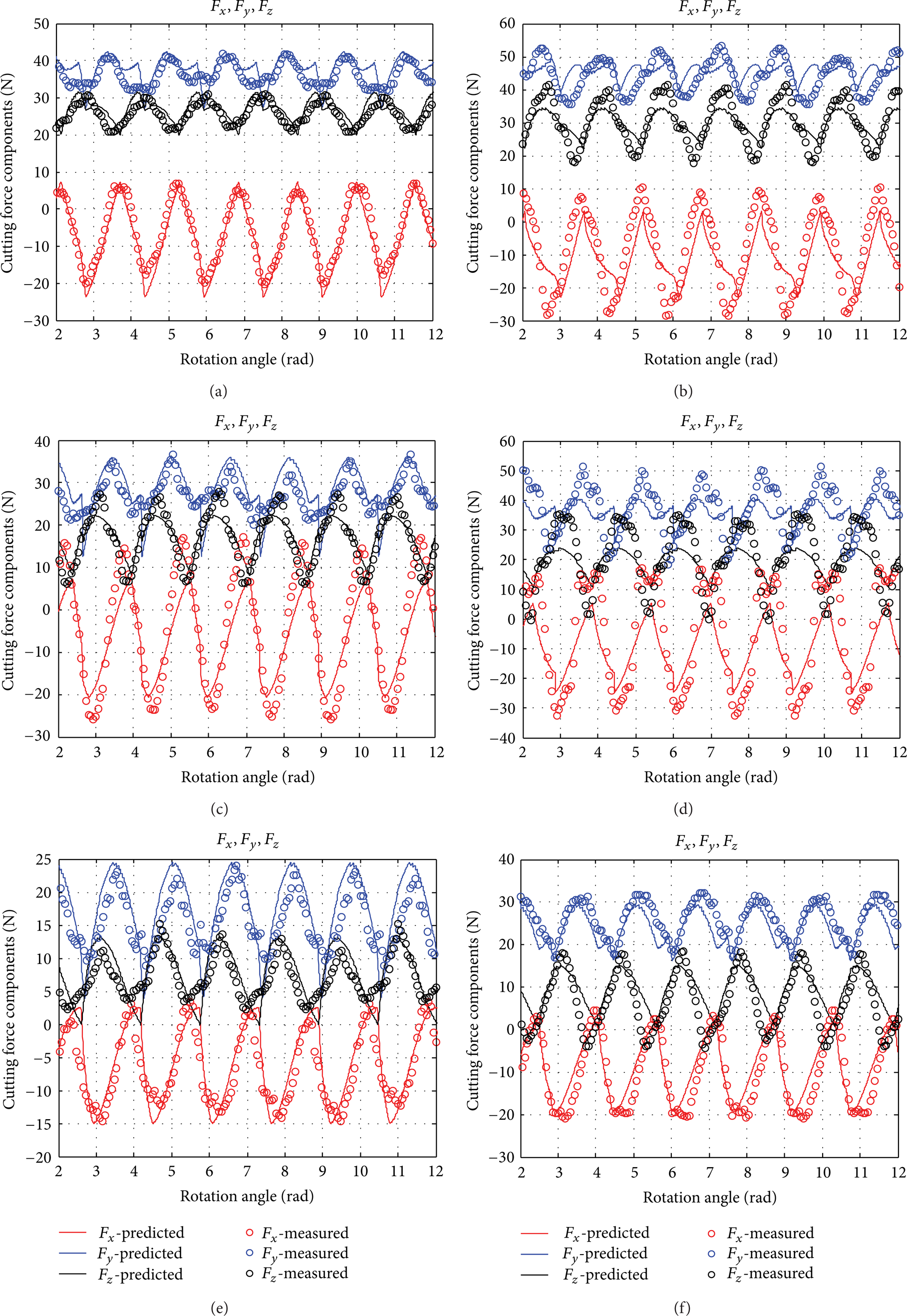
Comparison between predicted cutting forces and measured ones ((a) angle 10°, depth 0.4 mm; (b) angle 10°, depth 0.6 mm; (c) angle 15°, depth 0.4 mm; (d) angle 15°, depth 0.6 mm; (e) angle 20°, depth 0.4 mm; (f) angle 20°, depth 0.6 mm).

The figure illustrates six experiments, and each shows three force components in different cutting depths and inclination angles. Generally, experimental data has larger force range for the impact between the cutter and workpiece where FAM (Flute Average Method) can eliminate the run-out effects to some extent. From the coefficient formulations and start-exit angle data, it can be seen that both of them are either the function of cutting depth or relevant with cutting depth. When seeking for cutting forces, each disc of the cutter model has its corresponding coefficients which are different in discrete layer. Meanwhile, the number of discs can be used to control precision during force prediction but it may lead to longer time consumed in calculation. As for measured data, the same processing method is used as coefficients identification ones.

As can be observed from the results in the cutter revolution domain, influences of the inclination angle on measured and predicted cutting forces show a substantial agreement over large cutter rotating zone in terms of the amplitude, pulsation pattern, and period with slight differences. These deviations are inevitable for that the experiments have some uncontrollable factors such as vibration, the amount of coolant, temperature, and accuracy of workpiece fixture. And spindle speed is chosen in the stable zone based on the stability lobe diagram [22] to avoid chatter, while, in these cases, adopted cutting parameters such as lead angle may induce tool vibration and a hum during the machining can be the most convincing evidence of that. Regardless of these error sources, it has been proved that the predicted results give a relative accurate prediction of cutting forces in actual machining process which can be used to guide the parameter and condition optimization. This indicates that the hypotheses of the force model and coefficient identification approach are valid. Since the experiments are all about lead angle also known as inclination angle, in real machining situation, tilt angle can be also applied to obtain the desired surface. Particularly, the method of the tilt angle is similar to that of lead angle whatever the cutter oblique posture is.

Taking the condition of inclination angle with 20° and cutting depth with 0.4 mm as an example, the waveform deviation between measured and calculated data is small on F_x component (<10%), reasonable on F_y component (<20%), while more strenuous on F_z component (<25%) (Figure 14(a)). From the Figure, it can be get that the largest discrepancy remains at the peak-to-peak force region, while other simulated positions have reasonable values as measured. But a more amplitude offset appears in Figure 14(d). Offsets are mainly due to repetitive entries of cutting edges in workpiece which further causes instability. Also, some extent of edge, nose effects, and tool wear are accountable for the existing differences. Since the majority of predictions approximate to measured ones, they may be considered as acceptable prediction.

Figure 14:

Cutting force components comparison.

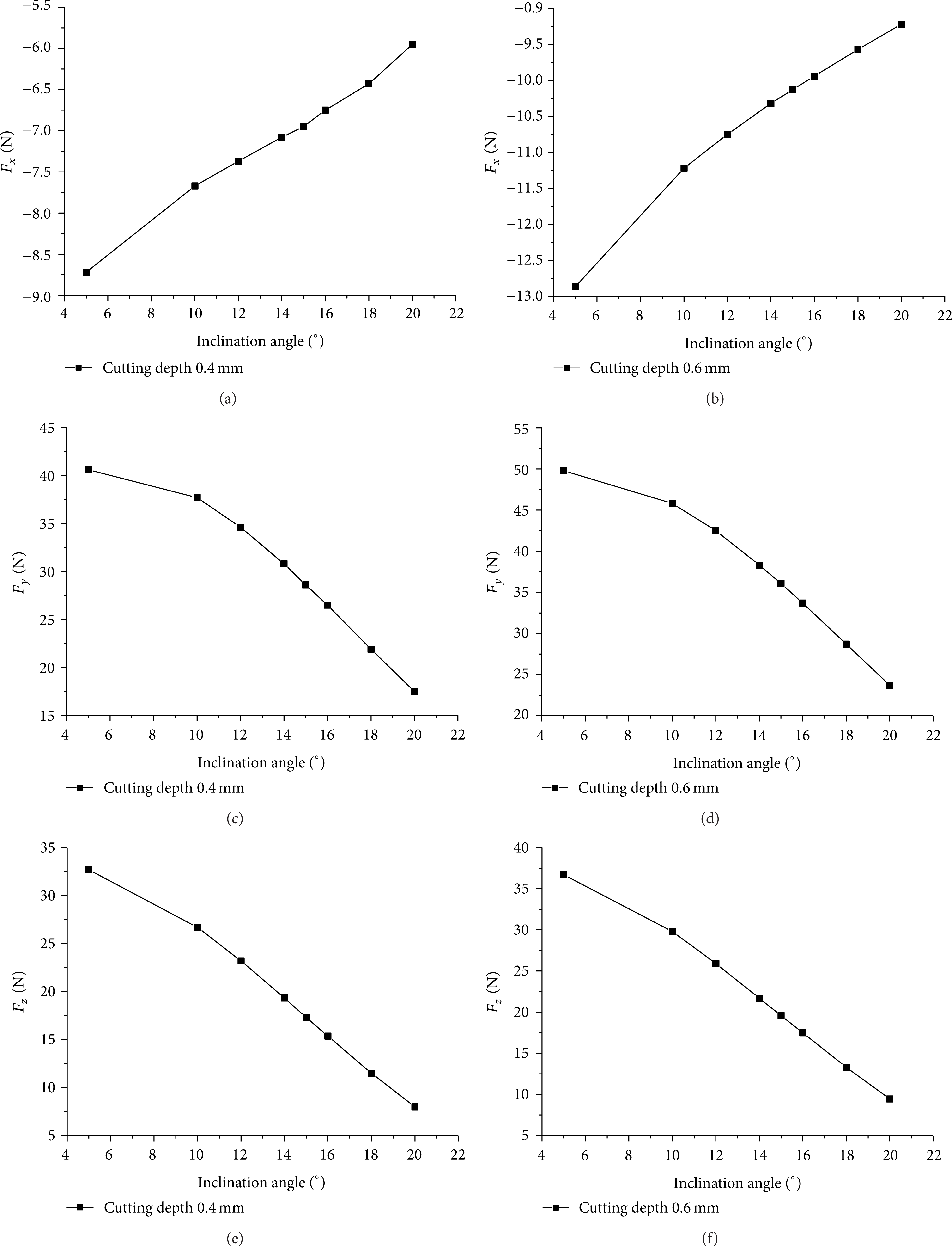
As different cutter inclination angles may affect the quantity of cutting forces, forces in this condition provide good basis for the solution of deformation, chatter, and so on. In actual applications, when deciding inclination angle, it usually takes geometric noninterference and uniform cutter orientation changing as principle and little information of physical parameter or this kind was thought. In CNC machining, cutter orientation can be the decisive element that affects engagement area; thus it is crucial to decrease perpendicular cutting force component and transverse force component on cutter.

Figure 14 illustrates the cutting forces along x-, y-, and z-axes under different inclination angles and cutting depths. It can be seen that when the inclination angle increases in a certain range, the cutting forces experience the same trend at the cutting depths of 0.4 mm and 0.6 mm. Nevertheless, the cutting force F_x appears to be in negative direction while F_y and F_z get the positive value. Therefore, a conclusion can be drawn that, on the condition that the surface quality and desired shape are maintained, we can choose the inclination angle based on cutting force components. For the exemplification, if the force on workpiece surface is tensile force, the residual stress involved in it may cause bad influence on the quality, lifespan, and so on. Thus, choosing the lead angle requires comprehensive consideration. These results indicate that, no matter in what milling strategy, if the cutting coefficients are determined in prior, the cutting force prediction can provide references and basis for the improvement of cutting stability and surface quality. Moreover, with the consideration of lead angle or tilt angle into cutting forces tendency, it offers a good way for optimizing inclination angle which further affects the efficiency and productivity.

7. Conclusions

In the adopted method for bull-nose end mill with inclination angles, cutting edges can be regarded as the division along tool axis into a number of equal distance discs. For each element and under different cutting speeds, it has independent cutting force coefficients derived through the semimechanistic coefficient identification method. The coefficients are supposed to be the function of each elemental elevation and start/exit angle. Then the start/exit angle is educed through engagement area acquisition by the geometry-based methodology, but it varies between discs regarded as the function of milling depth. All the experiment groups indicated the reasonable hypotheses and validation of the propositions where the measured cutting forces and predicted ones give an agreement in spite of some discrepancies. The deviations between them may be caused by either unstable factors in milling process or machine and device accuracy and other elements such as coolant, environmental temperature. The maximum deviation of average force for cases of steady cutting is smaller than 35% and the average error can be controlled in the range of 0–20%.

Based on the independence between adjacent layers, the coefficients at arbitrary layer have no relation with the previous neighbouring disc. Thus the current measured cutting forces should subtract the previous one which takes the recalculated results as input data. Specifically, traditional cutting force identification method was revised with respect to each cutting depth span; then, by fitting curve with z-axis distance as the horizontal coordinate, it made the force predictions more convenient and accurate with the aid of cubic polynomial fitting.

When the milling process has inclination angle between cutter axis and workpiece surface, it has a significant impact on cutting forces, among which start-exit angle plays an essential role. A geometric solution was represented with the aid of 3D software. It is assumed that the cutter geometry is the only input element on the condition that the workpiece was with straight surface. When the milling style is side milling with complex surface shape, the developed program can also make the solution possible by adding some modifications and real-time model refreshing. And the whole process can be time-efficient and result-effective. Although the experiments employed in the paper were aimed at lead angle and bull-nose mill, the method can be extended to tilt angle in sophisticated cutter posture, other milling cutters, and complicated workpiece surface. The model and approach are instructive for the optimization of cutting condition and parameters.

Conflict of Interests

The authors declare that they have no conflict of interests. The support of National Basic Research Program of China (Grant no. 2013CB035802), Basic Research Foundation of Northwestern Polytechnical University (Grant no. JCY20130121), and the 111 Project (Grant no. B13044) has no conflict of interests.

Footnotes

Acknowledgments

This work was sponsored by National Basic Research Program of China (Grant no. 2013CB035802), Basic Research Foundation of Northwestern Polytechnical University (Grant no. JCY20130121), and the 111 Project (Grant no. B13044).

References

Zheng

H. Q.

X. P.

Wong

Y. S.

, and Nee

A. Y. C.

, “Theoretical modelling and simulation of cutting forces in face milling with cutter runout,” International Journal of Machine Tools and Manufacture, vol. 39, no. 12, pp. 2003–2018, 1999.

Moufki

Dudzinski

Molinari

, and Rausch

, “Thermoviscoplastic modelling of oblique cutting: forces and chip flow predictions,” International Journal of Mechanical Sciences, vol. 42, no. 6, pp. 1205–1232, 2000.

Shin

Y. C.

and Waters

A. J.

, “A new procedure to determine instantaneous cutting force coefficients for machining force prediction,” International Journal of Machine Tools and Manufacture, vol. 37, no. 9, pp. 1337–1351, 1997.

Wan

Zhang

W. H.

Qin

G. H.

, and Tan

, “Efficient calibration of instantaneous cutting force coefficients and runout parameters for general end mills,” International Journal of Machine Tools and Manufacture, vol. 47, no. 11, pp. 1767–1776, 2007.

Feng

H.-Y.

and Su

, “A mechanistic cutting force model for 3D ball-end milling,” Journal of Manufacturing Science and Engineering, Transactions of the ASME, vol. 123, no. 1, pp. 23–29, 2001.

Gonzalo

Beristain

Jauregi

, and Sanz

, “A method for the identification of the specific force coefficients for mechanistic milling simulation,” International Journal of Machine Tools and Manufacture, vol. 50, no. 9, pp. 765–774, 2010.

Lee

H.-U.

and Cho

D.-W.

, “Development of a reference cutting force model for rough milling feedrate scheduling using FEM analysis,” International Journal of Machine Tools and Manufacture, vol. 47, no. 1, pp. 158–167, 2007.

X. P.

and Li

H. Z.

, “Theoretical modelling of cutting forces in helical end milling with cutter runout,” International Journal of Mechanical Sciences, vol. 46, no. 9, pp. 1399–1414, 2004.

Dabade

U. A.

Dapkekar

, and Joshi

S. S.

, “Modeling of chip-tool interface friction to predict cutting forces in machining of Al/SiCp composites,” International Journal of Machine Tools and Manufacture, vol. 49, no. 9, pp. 690–700, 2009.

10.

Wang

S.-M.

Chiou

C.-H.

, and Cheng

Y.-M.

, “An improved dynamic cutting force model for end-milling process,” Journal of Materials Processing Technology, vol. 148, no. 3, pp. 317–327, 2004.

11.

Engin

and Altintas

, “Mechanics and dynamics of general milling cutters. Part I: helical end mills,” International Journal of Machine Tools and Manufacture, vol. 41, no. 15, pp. 2195–2212, 2001.

12.

Gradišek

Kalveram

, and Weinert

, “Mechanistic identification of specific force coefficients for a general end mill,” International Journal of Machine Tools and Manufacture, vol. 44, no. 4, pp. 401–414, 2004.

13.

Azeem

Feng

H.-Y.

, and Wang

, “Simplified and efficient calibration of a mechanistic cutting force model for ball-end milling,” International Journal of Machine Tools and Manufacture, vol. 44, no. 2–3, pp. 291–298, 2004.

14.

Sun

and Guo

, “Numerical simulation and prediction of cutting forces in five-axis milling processes with cutter run-out,” International Journal of Machine Tools and Manufacture, vol. 51, no. 10–11, pp. 806–815, 2011.

15.

Ozturk

and Budak

, “Modeling of 5-axis milling processes,” Machining Science and Technology, vol. 11, no. 3, pp. 287–311, 2007.

16.

Ozturk

Tunc

L. T.

, and Budak

, “Investigation of lead and tilt angle effects in 5-axis ball-end milling processes,” International Journal of Machine Tools and Manufacture, vol. 49, no. 14, pp. 1053–1062, 2009.

17.

Moufki

Devillez

Dudzinski

, and Molinari

, “Thermomechanical modelling of oblique cutting and experimental validation,” International Journal of Machine Tools and Manufacture, vol. 44, no. 9, pp. 971–989, 2004.

18.

Fontaine

Moufki

Devillez

, and Dudzinski

, “Modelling of cutting forces in ball-end milling with tool-surface inclination. Part I: predictive force model and experimental validation,” Journal of Materials Processing Technology, vol. 189, no. 1–3, pp. 73–84, 2007.

19.

Fontaine

Devillez

Moufki

, and Dudzinski

, “Modelling of cutting forces in ball-end milling with tool-surface inclination. Part II. Influence of cutting conditions, run-out, ploughing and inclination angle,” Journal of Materials Processing Technology, vol. 189, no. 1–3, pp. 85–96, 2007.

20.

Kim

G. M.

Cho

P. J.

, and Chu

C. N.

, “Cutting force prediction of sculptured surface ball-end milling using Z-map,” International Journal of Machine Tools and Manufacture, vol. 40, no. 2, pp. 277–291, 2000.

21.

Cao

Zhao

Han

, and Chen

, “Force coefficients identification considering inclination angle for ball-end finish milling,” Precision Engineering, vol. 36, no. 2, pp. 252–260, 2012.

22.

Insperger

Gradišek

Kalveram

Stépán

Winert

, and Govekar

, “Machine tool chatter and surface location error in milling processes,” Journal of Manufacturing Science and Engineering, Transactions of the ASME, vol. 128, no. 4, pp. 913–920, 2006.

Prediction and Experimental Validation of Cutting Force for Bull-Nose End Mills with Lead Angle

Abstract

1. Introduction

2. Geometry of Bull-Nose End Mills

3. Mechanistic Cutting Force Model

4. Tool and Workpiece Engagement Area Acquisition

5. Identification of Specific Force Coefficients

6. Experimental Validation and Discussion

7. Conclusions

Conflict of Interests

Footnotes

Acknowledgments

References