Sage Journals: Discover world-class research

Abstract

Feedback contents of previous information feedback strategies in advanced traveler information systems are almost real-time traffic information. Compared with real-time information, prediction traffic information obtained by a reliable and effective prediction algorithm has many undisputable advantages. In prediction information environment, a traveler is prone to making a more rational route-choice. For these considerations, a mean velocity prediction information feedback strategy (MVPFS) is presented. The approach adopts the autoregressive-integrated moving average model (ARIMA) to forecast short-term traffic flow. Furthermore, prediction results of mean velocity are taken as feedback contents and displayed on a variable message sign to guide travelers' route-choice. Meanwhile, discrete choice model (Logit model) is selected to imitate more appropriately travelers' route-choice behavior. In order to investigate the performance of MVPFS, a cellular automaton model with ARIMA is adopted to simulate a two-route scenario. The simulation shows that such innovative prediction feedback strategy is feasible and efficient. Even more importantly, this study demonstrates the excellence of prediction feedback ideology.

1. Introduction

Advanced Traveler Information Systems (ATIS) are designed to provide real-time information regarding the traffic conditions for travelers. Generally, under the assistance of ATIS, travelers could make better route-choices. Without real-time information, travelers' route-choices are primarily based on experiential knowledge that is derived from learning of past experiences. As fundamental part of ATIS, the information feedback strategies have attracted great interest of transportation scholars [1 –4]. The aim of the information feedback strategies is to minimize individual road users' travel times and improve road service efficiency. Although people are full of expectation of ATIS, traffic condition would become more serious if an inappropriate information feedback strategy were to be adopted. It is still an essential task to find out an optimal and efficient information feedback strategy under ATIS [5 –7].

Accordingly, several conventional information feedback strategies have been proposed in recent years. These strategies mainly consist of three types: travel time feedback strategy (TTFS) [8], mean velocity feedback strategy (MVFS) [9], and congestion coefficient feedback strategy (CCFS) [10]. It has been proven that MVFS is more effective than TTFS, which is a lag effect approach and is impossible to provide travelers with the current situation of each route. In the meantime, CCFS is more effective than MVFS, the core of which is to define the congestion coefficient creatively [11]. Regardless of the fact that CCFS promotes the efficiency of the road networks, it needs higher detection precision and more computing resources of ATIS to compute the congestion coefficient. Based on above three strategies, Dong et al. [12, 13] put forward to a corresponding angle feedback strategy (CAFS), and a vehicle number feedback strategy (VNFS). Chen et al. [14 –16] put forward to a vehicle's length feedback strategy (VLFS), time flux feedback strategy (TFFS), and an exponential function feedback strategy (EFFS). Tobita and Nagatani [17] put forward to a tour-time feedback strategy. These information feedback strategies adopted various traffic flow feedback contents to evidently improve the capacity and performance of road networks.

Contents of the information feedback strategies are of two different types, namely, real-time and prediction feedback. However, all above-mentioned classic strategies almost adopted the former as major feedback factors. Compared with real-time information, prediction information obtained by some reliable prediction algorithm has many undisputable advantages. In particular, prediction information can reflect accurately short-term traffic flow conditions. In the prediction information circumstances, a traveler is prone to make a more reasonable route-choice [18, 19]. Nevertheless, only Dong et al. [20] took the lead in proposing to a prediction feedback strategy (PFS). Subsequently, they discussed the efficiency and superiority of PFS in three-route systems [21]. Their pioneering work convinced us of correctness and validity of prediction feedback ideology, but they could not rationally probe into details of the prediction method. In their research, the prediction information was calculated by means of pushing ahead the simulation system with the specified number of steps. It is ineffective that the later running results of traffic systems were adopted as feedback to guide current travelers' route-choices in practice.

On the other hand, some scholars pointed out that travelers' route-choice behavior was inconsistent with the principle of maximum utility theory (MUE), which is a conventional presumption to be taken for granted in the past research of information feedback strategies [22 –24]. Previous studies on feedback strategies could not take account of the complex relationship between route-choice behavior and real-time feedback information and purported that travelers would always choose the shortest-time route according to feedback information. Ben-Elia and Shiftan [25] suggested that travelers should make route-choice relying on both real-time information and their historical experience. Bekhor and Albert [26] demonstrated that certain sensation seeking domains alongside traditional variables played an important role in route-choice behavior with pretrip travel time information. It demands that we should introduce another more practical route-choice model than MUE to imitate travelers' route-choice behavior. Furthermore, Niu and Zhou [27] proposed a dynamic traffic demand driven idea to solve urban traffic problem, and they studied the optimizing urban rail timetable by this advantageous notion. Compared with conventional fixed traffic demand, the dynamic traffic demand driven idea is more practical.

The purpose of this study is to find an accurate and feasible prediction algorithm for prediction feedback strategies in terms of realistic traffic conditions. In our study, the autoregressive-integrated moving average model (ARIMA) is adopted to forecast traffic flow conditions, and the discrete choice model is chosen to imitate traveler's route-choice behavior rather than MUE. Mean velocity selected from several parameters of traffic flow such as travel-time, flux, density and velocity, is used for prediction object of ARIMA, because it is typical of traffic conditions. Moreover, performance analysis of such mean velocity prediction information feedback strategy (MVPFS) in two-route scenario is expounded.

The remainder of this paper is organized as follows. In Section 2, traffic flow characteristic is investigated in order to build a proper prediction model of traffic flow, and ARIMA prediction modeling framework is depicted in detail on the basis of two-route scenario. In Section 3, we present factual simulation results and analyze the results concerning the comparison of MVFS. In the ending section, we work out some conclusions and suggestions.

2. Mean Velocity Prediction Information Feedback Strategies

2.1. Traffic Flow Characteristic

A traffic flow system mainly composed of people, vehicles, and roads is commonly regarded as a time-varying complex nonlinear system. As an important research method in nonlinear computational science, the cellular automata model is very applicable to imitate a space-time evolutionary process of microcosmic traffic flow systems dynamically [28, 29].

Compared with the NS mechanism that is the most popular and simplest cellar automaton model to investigate the traffic flow, the VDR mechanism is a more functional one in analyzing the traffic flow [30], which considers the velocity dependence of random brake p. In this model, due to the variables of discrete time and space, the road is subdivided into cells of length 7.5 m, and the vehicles update their positions and velocities according to the following rules:

acceleration: v_n(t) → v_n(t + 1/3) = min ⁡ {v_n(t) + 1, V_{max ⁡}};

deceleration: v_n(t + 1/3) → v_n(t + 2/3) = min ⁡ {v_n(t + 1/3), d_n(t)};

randomization with probability P_n(t + 1):

\begin{matrix} P_{n} (t + 1) = \{\begin{cases} P_{0}, & v_{n} (t) = 0; \\ P_{d}, & v_{n} (t) > 0, \end{cases} \\ v_{n} (t + \frac{2}{3}) ⟶ v_{n} (t + 1) = \max \{v_{n} (t + \frac{2}{3}) - 1,0\}; \end{matrix}

(1)

vehicle motion: x_n(t + 1) = x_n(t) + v_n(t + 1).

Where v_n(t) is the speed of the nth vehicle at time t; V_{max ⁡} denotes the maximal velocity of vehicles; d_n(t) is defined to be the number of empty cells in front of the nth vehicle at time t; x_n(t) is the location of the nth vehicle at time t; P₀ and P_d denote the probabilities of randomization according to vehicle's velocity at time t, and P_d is smaller than P₀.

2.2. Two-Route Scenario

The two-route scenario was investigated by Wahle et al. [8] in which travelers chose one of the two routes according to the feedback information displayed on a variable message sign (VMS), located at the entrance of routes (see Figure 1). In the two-route scenario, it is supposed that there are two routes A and B of the same length L. The concept of three-route systems, which contains three routes of the same length, is analogous with the situation of two-route systems.

Figure 1:

The two-route scenario.

At every time step, a new vehicle is generated at the entrance of two-route system and will choose one route (A or B) according to VMS. If a new vehicle enters the desired route, it will be subjected to the rules of VDR model on the route. Conversely, if a new vehicle is unable to enter the desired route, it will be deleted. The vehicle will be removed after it reaches the end point of the route. An overall procedure of the feedback strategy is given as follows. Initially, two routes and VMS are empty, and new vehicles choose route l (l is A or B) randomly. After the prespecified time step, prediction feedback information will be computed based on real-time traffic data and displayed on the VMS at each time step.

As a rule, traffic conditions of one route could be characterized by density, mean velocity, and flux, which are defined as follows:

\begin{matrix} ρ = \frac{N}{L}, \\ \bar{v} = \frac{\sum_{n = 1}^{N} v_{n}}{N}, \\ f = \bar{v} \cdot ρ = \frac{\sum_{n = 1}^{N} v_{n}}{L}, \end{matrix}

(2)

where ρ represents the traffic density on one route; $\bar{v}$ represents the mean velocity of all vehicles on one route; f represents the flux on one route; N is the vehicle number on one route; v_n is the speed of the nth vehicle on one route. Among three parameters, $\bar{v}$ is so typical that it can be utilized to represent partly road conditions.

2.3. ARIMA Prediction Model

2.3.1. Modeling

If we set up a random variable X_t to represent the mean velocity of all vehicles on one route at time t, {X_t} (t = 1,2, 3, …, m) would structure a time series. The values of X_t are constantly changeable with time, but not necessarily strict function of time. The values of this time series are affected partly by various accidental factors and show up highly randomicity and distinct nonstationary. But the more important thing is there is a certain statistical correlation among the time sequences. It can be deduced that {X_t} is a nonstationary stochastic time series, so we can build a rational statistical model to interpret statistical regularity in the time sequences [31]. It is the statistical model that makes it possible to forecast short-term traffic flow. Smith et al. [32] and Min and Wynter [33] expounded the role and steps of ARIMA for short-term traffic flow forecasting. In time series analysis, ARIMA is an effective approach to find the best fit of a time series to past values of this time series, in order to make forecasts.

ARIMA model takes historical data into account and decomposes it into an Autoregressive (AR) process; an Integrated (I) process, which accounts for differential stationarizing to preprocess the original nonstationary stochastic time series; and a Moving Average (MA) of the forecast errors, such that the longer the historical data, the more accurate the forecast will be, as it learns over time. There are three parameters (p, d, q) interacting each other in ARIMA model. Where p is the number of autoregressive; d is the number of differences; q is the number of moving average terms [34, 35].

Before building ARIMA model, we should adopt zero mean normalization and differential stationarizing method to preprocess the original nonstationary stochastic time series. The reason for data preprocessing is that the unique object for ARIMA model is zero mean value stationary stochastic time series. Such zero mean normalization method and the differential stationarizing method (only given first order and the rest may be deduced by analogy) are expressed by (3) and (4), respectively:

X_{t}^{'} = X_{t} - \frac{1}{m} \sum_{i = 1}^{m} X_{i},

(3)

\nabla X_{t}^{'} = X_{t}^{'} - X_{t - 1}^{'}, t > 1,

(4)

where X_t^′ represents the result of zero mean normalization, and {X_t^′} are a new time series; m is the length of original time series; ∇X_t^′ represents the result of differential stationarizing, and {∇X_t^′} are a zero mean value stationary stochastic time series, which are the input data of ARIMA model. Just to be clear, we set up another stochastic time series {Y_t} (1 < t ≤ m) to represent {∇X_t^′}.

The general form of ARIMA (p, d, q) model is expressed as

Y_{t} = c + ε_{t} + \sum_{i = 1}^{p} φ_{i} Y_{t - i} + \sum_{i = 1}^{q} θ_{i} ε_{t - i},

(5)

where ϕ = (ϕ₁, ϕ₂, …, ϕ_p)^T are parameters of the autoregressive part; θ = (θ₁, θ₂, …θ_q)^T are parameters of the moving average part; c is a constant; ∊_t is white noise series, which are generally assumed to be independent, identically distributed variables sampled from a normal distribution with zero mean, namely, ∊_t ~ N(0, σ²).

The best linear forecast is a necessary concept to implement forecasting in ARIMA. We set up that B and A_j (1 ≤ j ≤ m) are random variables of zero mean value and bounded variance. For a ∈ Ω and ∀b ∈ Ω, the inequality (6) is valid. Then, a^TA is just called the best linear forecast for B using A₁, A₂, …, A_m, denoted by L(B∣A) or $\hat{B}$ . Thereupon, the formula $\hat{B} = L (B ∣ A) = a^{T} A$ can be used

E {(B - a^{T} A)}^{2} \leq E {(B - b^{T} A)}^{2} .

(6)

On the basis of the above analysis, ${\hat{Y}}_{m + 1}$ is to be forecasted by

{\hat{Y}}_{m + 1} = \{\begin{cases} \sum_{i = 1}^{m} θ_{m, i} Z_{m + 1 - i}, & 1 \leq m < r, \\ \sum_{i = 1}^{p} φ_{i} Y_{m + 1 - i} + \sum_{i = 1}^{q} θ_{m, i} Z_{m + 1 - i}, & m \geq r, \end{cases}

(7)

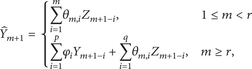
where r = max ⁡ (p, q); Z_t = Y_t − L(Y_t∣Y_{t − 1}) and Z₁ = Y₁; θ_{m + k, i} is a parameter that can be obtained by recursive formula

\begin{matrix} s_{0} = γ_{0}, \\ θ_{m, m - k} = \frac{(γ_{m - k} - \sum_{i = 0}^{k - 1} θ_{k, k - i} θ_{m, m - i} s_{i})}{s_{k}}, 0 \leq k \leq m - 1, \\ s_{m} = γ_{m + 1} - \sum_{i = 0}^{m - 1} θ_{m, m - i}^{2} s_{i}, \end{matrix}

(8)

where γ_l is autocovariance function; it can be calculated by

γ_{l} = \frac{1}{m} \sum_{i = 1}^{m - l} Y_{i + l} Y_{i}, 0 \leq l < m .

(9)

2.3.2. Prediction Steps

The following gives a brief description of the prediction algorithm.

Step 1 (Identification). This process aims to find the best-fit values of parameters (p, d, q) for the time series data. The value of parameter d represents the number of differences for time series {X_t}. Once {X_t} has been rendered stationary by differencing, the choice of p and q may be made by examining two time-domain constructs: the autocorrelation function (ACF) and the partial autocorrelation function (PACF). Specifically, values of parameters p and q could be decided by akaike information criterion (AIC). Supposing that P₀ is upper bound of p and Q₀ is upper bound of q, for ∀(k, j), 0 ≤ k ≤ P₀ and 0 ≤ j ≤ Q₀ are valid. Thus, the value of AIC function can be calculated by

AIC (k, i) = \ln ({\hat{σ}}^{2} (k, i)) + \frac{2 (k + i)}{m},

(10)

where ${\hat{σ}}^{2}$ is an estimated value of σ² which is the variance of white noise series ∊_t. Since then, the minimum point $(\hat{p}, \hat{q})$ of AIC(k, i) is called AIC fixed-order of (p, q).

Step 2 (Estimation). Once the parameters (p, d, q) are determined, next step is to estimate all autoregressive and moving average parameters in ARIMA model. The least square method is a popular choice for parameter estimation.

Step 3 (Diagnostic checking). It is a necessary step to make reasonableness check for the preliminary ARIMA (p, d, q) model, which is just built by Steps 1 and 2. If the check results meet the requirements, we can accept this preliminary fitting model. If not, we should return step 1 and refit the model, until the check results are compatible.

Step 4 (Forecasting). We can use the ARIMA model that has accomplished the first three steps to forecast X_{m + 1}, which represents the mean velocity of all vehicles on one route at time m + 1. Furthermore, X_{m + η} (η ∈ [1, h]) could be obtained by the recursive method. Where η is a certain time of future; h is the maximum prediction period.

2.3.3. Prediction Information Feedback

After obtaining the forecasting series {X_{m + η}}, we can calculate the mean value of {X_{m + η}}. And then, such mean value about route l can be denoted as F_l, which indicates short-term traffic conditions regarding route l. It is F_l that would be displayed on VMS as feedback information.

2.4. Route-Choice Model

Acquiring the prediction feedback information F_l displayed on VMS, travelers will make route-choices according to the Logit model. In this model, travelers would choose route l with a probability p_l as

p_{l} = \frac{\exp (λ F_{l})}{\sum_{l^{'} \in \{A, B\}}^{} \exp (λ F_{l^{'}})},

(11)

where λ ∈ [0, + ∞) denotes the rational degree of travelers. When λ = 0, the probability of choosing one route is equal to that of another route and it is 1/2. When λ → + ∞, traveler's choice is the optimal route.

2.5. Processing Procedures

Figure 2 shows a schematic diagram of the mean velocity prediction information feedback strategy, which demonstrates the affecting mechanism of information feedback.

Figure 2:

The schematic diagram of prediction feedback.

3. Simulation Results and Discussions

In simulations, the length of two-route L is 1000 cells; the maximal velocity V_{max ⁡} is set to be 4; the randomization break probability is P₀ = 0.5 and P_d = 0.25. In the route-choice model, we set λ = 3.5. Before verifying performance of MVPFS, we should fix the ARIMA model parameters (p, d, q) firstly. Testing and calculating by using historical simulation traffic data generated from VDR model, we could confirm that the best-fit values of (p, d, q) are (1,1, 2).

All simulation results of flux, velocity, and vehicle number are obtained by 60000 iterations excluding the initial 50000 time steps. We compared MVPFS with MVFS under the same condition in order to reveal characters of the new strategy. In addition, we investigated the relationship between the performance and the prediction periods, including 100, 200, and 300.

Figure 3 displays the changing of flux of each route according to time when adopting the four kinds of feedback strategies. Regardless of feedback strategies, the numbers of vehicles passing through the entire two-route system are approximately equal. There is nevertheless a perceptible difference in intermittent oscillation frequency between real-time and prediction feedback. The intermittent oscillation frequency of real-time feedback is more violent than that of prediction feedback, and it manifests that prediction feedback can suppress the intermittent oscillation frequency more effectively.

Figure 3:

The flux of each route with (a) MVFS, (b) MVPFS with 100 periods, (c) MVPFS with 200 periods, and (d) MVPFS with 300 periods.

Figure 4 illustrates the changing of mean velocity of each route according to time when adopting the four kinds of feedback strategies. There are distinct differences among these strategies. Firstly, the variation range of prediction feedback is obviously smaller than that of real-time feedback; secondly, the intermittent oscillation frequency of prediction feedback is perceptible lower than that of real-time feedback; lastly and most importantly, the average velocity of prediction feedback is evidently higher than that of real-time feedback.

Figure 4:

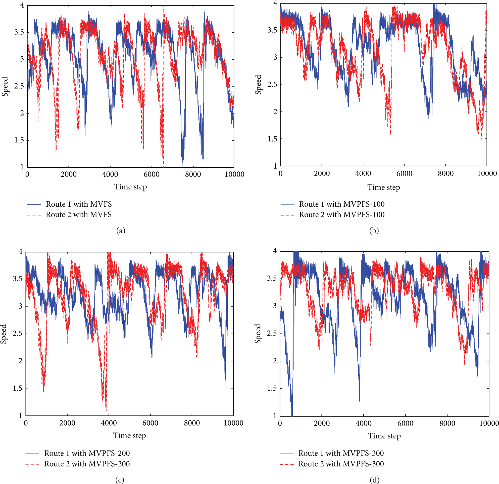
The average speed of each route with (a) MVFS, (b) MVPFS with 100 periods, (c) MVPFS with 200 periods, and (d) MVPFS with 300 periods.

Figure 5 illustrates the changing of vehicle's number of each route according to time when adopting the four kinds of feedback strategies. On the whole, there are no significant differences between prediction feedback and real-time feedback. It means there are basically the same densities among four strategies.

Figure 5:

The vehicle number of each route with (a) MVFS, (b) MVPFS with 100 periods, (c) MVPFS with 200 periods, and (d) MVPFS with 300 periods.

Therefore, we can deduce that the prediction feedback strategy is superior to the real-time feedback strategy. In addition, there is a particular concern that is the complex relationship between performance of strategy and prediction periods. Performance of feedback strategies seems intuitively to be greatly affected by prediction periods. But this is not the case. The reason may be that more prediction periods have only a modest impact on the travelers' route-choice. Of course, precision of traffic prediction may be part of the reason.

The statistical analysis of simulation results is to be demonstrated in Table 1. It is known that travel time is a dominant factor for road users making route-choice. We can see clearly from Table 1 that the average travel time of MVFS is longer than those adopting prediction feedback strategies. When adopting the prediction feedback strategies, we can better realize traffic assignment, so as to alleviate traffic congestion. In prediction feedback strategies, the strategy with 300 periods is superior to the rest two strategies a little. But, more computing resource is consumed in vain. Thus, we can comprehend that the prediction periods has limited effect on the performance of prediction feedback strategies.

Table 1:

Numerical analysis of simulation data.

	MVFS	MVPFS(100 periods)	MVPFS(200 periods)	MVPFS(300 periods)

Flux of route 1	0.3014	0.3288	0.3239	0.2815
Flux of route 2	0.3007	0.3289	0.3025	0.3298
Average speed of route 1	3.0670	3.1945	3.2438	3.1512
Average speed of route 2	3.0671	3.1386	3.1946	3.3120
Vehicle number of route 1	97.9056	105.4888	100.4978	91.3871
Vehicle number of route 2	97.4139	107.0167	95.3904	100.4850

Average flux of two routes	0.3010	0.3288	0.3132	0.3056
Average speed of two routes	3.0671	3.1666	3.2192	3.2316
Average vehicle number of two routes	97.6598	106.2528	97.9441	95.9361
Average travel time	326.0453	315.8002	310.6371	309.4441

4. Conclusions

By the aid of ATIS, we studied the approach about how to use prediction information in feedback strategies. In this study, we proposed a feasible and effective prediction information feedback approach—the mean velocity prediction information feedback strategy. On the basis of traffic flows characteristic analysis, the autoregressive-integrated moving average model was adopted to forecast traffic flow conditions, which is an excellent prediction method in stochastic time series analysis. Both the selection of prediction object and the whole prediction procedure were discussed in detail. VDR model was adopted to verify the performance of this prediction feedback strategy. Simulation showed that prediction feedback was more advantageous to route-choices of all travelers.

Compared with the mean velocity feedback strategy, new strategy can reduce travel time of travelers and promote utilization efficiency of road networks palpably. Although the prediction periods have limited effect on the performance of feedback strategies, we suggest that more periods should be adopted if possible. In the further research, we are going to find more precise prediction algorithm and endeavor to reveal the complex relationship between performance of feedback strategies and prediction periods.

Conflict of Interests

The authors declare that there is no conflict of interests regarding the publication of this paper.

Footnotes

Acknowledgments

This research work is supported by the Humanity and Social Science Youth foundation of Ministry of Education in China (Grant no. 12YJC630200), the Natural Science Foundation of Gansu Province in China (Grant no. 145RJZA190), and the Social Science Planning Project of Gansu Province in China (Grant no. 13YD066).

References

Tang

J. J.

Wang

Y. H.

Wang

, and Liu

, “Complex network approach for the complexity and periodicity in traffic time series,” Procedia—Social and Behavioral Sciences, vol. 96, pp. 2602–2610, 2013.

Bekhor

and Albert

, “Accounting for sensation seeking in route choice behavior with travel time information,” Transportation Research Part F: Traffic Psychology and Behaviour, vol. 22, pp. 39–49, 2014.

Gao

Frejinger

, and Ben-Akiva

, “Cognitive cost in route choice with real-time information: an exploratory analysis,” Transportation Research Part A: Policy and Practice, vol. 45, no. 9, pp. 916–926, 2011.

Cristea

and Delhomme

, “Comprehension and acceptability of on-board traffic information: beliefs and driving behaviour,” Accident Analysis & Prevention, vol. 65, pp. 123–130, 2014.

Ben-Elia

Ishaq

, and Shiftan

, “If only I had taken the other road…”: regret, risk and reinforced learning in informed route-choice,” Transportation, vol. 40, no. 2, pp. 269–293, 2013.

Levinson

and Zhu

, “A portfolio theory of route choice,” Transportation Research Part C: Emerging Technologies, vol. 35, pp. 232–243, 2013.

Zhang

and Gao

Z. Y.

, “Effect of ATIS information under incident-based congestion propagation,” Procedia—Social and Behavioral Sciences, vol. 43, pp. 628–637, 2012.

Wahle

Bazzan

A. L. C.

Klügl

, and Schreckenberg

, “Decision dynamics in a traffic scenario,” Physica A: Statistical Mechanics and its Applications, vol. 287, no. 3–4, pp. 669–681, 2000.

Lee

Hui

P.M.

Wang

B.-H.

, and Johnson

N. F.

, “Effects of announcing global information in two-route traffic flow model,” Journal of the Physical Society of Japan, vol. 70, no. 12, pp. 3507–3510, 2001.

10.

Wang

W.-X.

Wang

B.-H.

Zheng

W.-C.

Yin

C.-Y.

, and Zhou

, “Advanced information feedback in intelligent traffic systems,” Physical Review E, vol. 72, no. 6, Article ID 066702, 2005.

11.

Zhao

X.-M.

Xie

D.-F.

Gao

Z.-Y.

, and Gao

, “Equilibrium of a two-route system with delayed information feedback strategies,” Physics Letters A, vol. 377, no. 43, pp. 3161–3169, 2013.

12.

Dong

C. F.

and Ma

, “Corresponding Angle Feedback in an innovative weighted transportation system,” Physics Letters Section A, vol. 374, no. 24, pp. 2417–2423, 2010.

13.

Dong

C. F.

, and Wang

B. H.

, “Effects of vehicle number feedback in multi-route intelligent traffic systems,” International Journal of Modern Physics C, vol. 21, no. 8, pp. 1081–1093, 2010.

14.

Chen

Xie

Tong

Dong

Shi

, and Wang

, “A comprehensive study of advanced information feedbacks in real-time intelligent traffic systems,” Physica A: Statistical Mechanics and Its Applications, vol. 391, no. 8, pp. 2730–2739, 2012.

15.

Chen

B.-K.

Tong

Zhang

W.-Y.

Sun

X.-Y.

, and Wang

B.-H.

, “Flux information feedback strategy in intelligent traffic systems,” Europhysics Letters, vol. 97, no. 1, Article ID 14001, 2012.

16.

Chen

B. K.

Dong

C. F.

Liu

Y. K.

, “Real-time information feedback based on a sharp decay weighted function,” Computer Physics Communications, vol. 183, no. 10, pp. 2081–2088, 2012.

17.

Tobita

and Nagatani

, “Effect of signals on two-route traffic system with real-time information,” Physica A, vol. 391, no. 23, pp. 6137–6145, 2012.

18.

Chrobok

Kaumann

Wahle

, and Schreckenberg

, “Different methods of traffic forecast based on real data,” European Journal of Operational Research, vol. 155, no. 3, pp. 558–568, 2004.

19.

Svenson

Eriksson

Salo

, and Peters

, “Judgments of mean speed and predictions of route choice,” Transportation Research Part F, vol. 14, no. 6, pp. 504–511, 2011.

20.

Dong

C.-F.

Wang

G.-W.

Sun

X.-Y.

, and Wang

B.-H.

, “Prediction feedback in intelligent traffic systems,” Physica A: Statistical Mechanics and its Applications, vol. 388, no. 21, pp. 4651–4657, 2009.

21.

Dong

Wang

, and Sun

, “Effects of prediction feedback in multi-route intelligent traffic systems,” Physica A: Statistical Mechanics and Its Applications, vol. 389, no. 16, pp. 3274–3281, 2010.

22.

Shiftan

Bekhor

, and Albert

, “Route choice behaviour with pre-trip travel time information,” IET Intelligent Transport Systems, vol. 5, no. 3, pp. 183–189, 2011.

23.

Prato

C. G.

Bekhor

, and Pronello

, “Latent variables and route choice behavior,” Transportation, vol. 39, no. 2, pp. 299–319, 2012.

24.

Gao

, “Modeling strategic route choice and real-time information impacts in stochastic and time-dependent networks,” IEEE Transactions on Intelligent Transportation Systems, vol. 13, no. 3, pp. 1298–1311, 2012.

25.

Ben-Elia

and Shiftan

, “Which road do i take? A learning-based model of route-choice behavior with real-time information,” Transportation Research Part A, vol. 44, no. 4, pp. 249–264, 2010.

26.

Bekhor

and Albert

, “Accounting for sensation seeking in route choice behavior with travel time information,” Transportation Research F: Traffic Psychology and Behavior, vol. 22, pp. 39–49, 2014.

27.

Niu

and Zhou

, “Optimizing urban rail timetable under time-dependent demand and oversaturated conditions,” Transportation Research Part C: Emerging Technologies, vol. 36, pp. 212–230, 2013.

28.

Maerivoet

and DeMoor

, “Cellular automata models of road traffic,” Physics Reports, vol. 419, no. 1, pp. 1–64, 2005.

29.

H.-X.

Zhu

H.-B.

, and Dai

S.-Q.

, “Cellular automaton traffic flow model considering intelligent transportation system,” Acta Physica Sinica, vol. 54, no. 10, pp. 4621–4626, 2005.

30.

Barlovic

Santen

Schadschneider

, and Schreckenberg

, “Metastable states in cellular automata for traffic flow,” The European Physical Journal B: Condensed Matter and Complex Systems, vol. 5, no. 3, pp. 793–800, 1998.

31.

Ishak

and Al-Deek

, “Performance evaluation of short-term time-series traffic prediction model,” Journal of Transportation Engineering, vol. 128, no. 6, pp. 490–498, 2002.

32.

Smith

B. L.

Williams

B. M.

, and Keith Oswald

, “Comparison of parametric and nonparametric models for traffic flow forecasting,” Transportation Research C: Emerging Technologies, vol. 10, no. 4, pp. 303–321, 2002.

33.

Min

W. L.

and Wynter

, “Real-time road traffic prediction with spatio-temporal correlations,” Transportation Research Part C, vol. 19, no. 4, pp. 606–616, 2011.

34.

Williams

B. M.

Durvasula

P. K.

, and Brown

D. E.

, “Urban freeway traffic flow prediction: application of seasonal autoregressive integrated moving average and exponential smoothing models,” Transportation Research Record, no. 1644, pp. 132–141, 1998.

35.

Asteriou

and Hall

S. G.

, “ARIMA models and the box-jenkins methodology,” in Applied Econometrics, pp. 265–286, Palgrave MacMillan, 2nd edition, 2011.

Mean Velocity Prediction Information Feedback Strategy in Two-Route Systems under ATIS

Abstract

1. Introduction

2. Mean Velocity Prediction Information Feedback Strategies

2.1. Traffic Flow Characteristic

2.2. Two-Route Scenario

2.3. ARIMA Prediction Model

2.3.1. Modeling

2.3.2. Prediction Steps

2.3.3. Prediction Information Feedback

2.4. Route-Choice Model

2.5. Processing Procedures

3. Simulation Results and Discussions

4. Conclusions

Conflict of Interests

Footnotes

Acknowledgments

References