
Abstract
Sonar signals recognition is an important task in detecting the presence of some significant objects under the sea. In military, sonar signals are used in lieu of visuals to navigate underwater and/or locate enemy submarines in proximity. In particular, classification algorithm in data mining has been applied in sonar signal recognition for recognizing the type of surfaces from which the sonar waves are bounced. Classification algorithms in traditional data mining approach offer fair accuracy by training a classification model with the full dataset, in batches. It is well known that sonar signals are continuous and they are collected as data streams. Although the earlier classification algorithms are effective in traditional batch training, it may not be practical for incremental classifier learning. Since sonar signal data streams can amount to infinity, the data preprocessing time must be kept to a minimum to fulfill the need for high speed. This paper presents an alternative data mining strategy suitable for the progressive purging of noisy data via fast conflict analysis from the data stream without the need to learn from the whole dataset at one time. Simulation experiments are conducted and superior results are observed in supporting the efficacy of the methodology.
1. Introduction
In general, sonar which stands for sound navigation and ranging is a sound propagation technology used in underwater navigation, communication, and/or detection of submarine objects. The relevant techniques have been recently reviewed in [1]. In particular, it was highlighted that detection/classification task of sonar signals is one of the most challenging topics in the field.
Choosing the right classification model for sonar signals recognition is an important matter in detecting the presence of objects of interest under the sea. As it was pointed out in [2], underwater sensor networks support a variety of applications, such as ocean sampling networks, environment monitoring, offshore explorations, disaster prevention, assisted navigation, and mine reconnaissance. Underwater sensor networks are easy to deploy and eliminate the need of cables, and they do not interfere with shipping activity. However, sonar signals that propagate underwater especially in long haul are prone to noise and interferences. In particular, classification techniques in data mining have been employed widely in sonar signal recognition to distinguish the surface of the target object from which the sonar waves are echoed [3–5].
Classification algorithms in traditional data mining approach may be able to achieve substantial accuracy by inducing a classification model using the whole dataset. The induction however is usually done and repeated in batches, which implies certain decline in accuracy between the models updates which may be expected [6]. Moreover, the update time may become increasingly long as the whole bulk of dataset gets larger when fresh data accumulates. Just like any data stream, it is known that sonar signals are incessant and they are sensed in continual manner. Even though the batch-mode classification algorithms produce an accurately trained model, it may not be suitable in streaming scenarios such as sonar sensing. Since sonar signal data streams can potentially sum to infinity, it is crucial to keep the data processing time very short for real-time sensing and scouting.
In this paper, we present an alternative data stream mining methodology designed for the incrementally purging of noisy data using fast conflict analysis from the stream-based training dataset. It is called incremental data stream mining methodology with conflict analysis or iDSM-CA (in acronym). The methodology has an advantage of learning a classification model from the stream data incrementally. Simulation experiments are carried out to illustrate the efficacy of the proposed methodology, especially in overcoming the task of removing noisy data from the sonar data while they are streaming.
The rest of the paper is organized as follows. Section 2 highlights some popular computational techniques for the detection and removal of noise from training datasets. Section 3 describes our new data stream mining approach and the “conflict analysis” mechanism used for removing misclassified instances. Section 4 presents a series of sonar recognition experiments for validating the stream mining approach. Section 5 concludes the paper.
2. Related Work
Researchers have attempted different techniques for detecting and removing noisy data, which are generally referred to as random chaos in the training dataset. Basically, these techniques identify data instances that confuse the training model and diminish the classification accuracy. In general, they look for data irregularities and how they do affect classification performance. Most of these techniques can fit under these three categories: statistics-based, similarity-based, and classification-based methods.
2.1. Statistics-Based Noise Detection Methods
Outliers, or data with extraordinary values, are interpreted as noise in this kind of method. Detection techniques proposed in the literature range from finding extreme values beyond a certain number of standard deviations to complex normality tests. Comprehensive surveys of outlier detection methods used to identify noise in preprocessing can be found in [7, 8]. In [9], the authors adopted a special outlier detection approach in which the behavior projected by the dataset is checked. If a point is sparse in a lower low-dimensional projection, the data it represents are deemed abnormal and are removed. Brute force, or at best, some form of heuristics, is used to determine the projections.
A similar method outlined by [10] builds a height-balanced tree containing clustering features on nonleaf nodes and leaf nodes. Leaf nodes with a low density are then considered outliers and are filtered out.
2.2. Similarity-Based Noise Detection Methods
This group of methods generally requires a reference by which data are compared to measure how similar or dissimilar they are to the reference.
In [11], the researchers first divided data into many subsets before searching for the subset that would cause the greatest reduction in dissimilarity within the training dataset if removed. The dissimilarity function can be any function returning a low value between similar elements and a high value between dissimilar elements, such as variance. However, the authors remarked that it is difficult to find a universal dissimilarity function. Xiong et al. [12] proposed the HCleaner technique applied through a hyperclique-based data cleaner. Every pair of objects in a hyperclique pattern has a high level of similarity related to the strength of the relationship between two instances. The HCleaner filters out instances excluded from any hyperclique pattern as noise. Another team of researchers [13] applied a k-NN algorithm, which essentially compares test data with neighboring data to determine whether they are outliers by reference to their neighbors. By using their nearest neighbors as references, different data are treated as incorrectly classified instances and removed. The authors studied patterns of behavior among data to formulate Wilson's editing approach, a set of rules that automatically select the data to be purged.
2.3. Classification-Based Noise Detection Methods
Classification-based methods are those that rely on one or more preliminary classifiers built as references for deciding which data instances are incorrectly classified and should be removed.
In [14], the authors used an n-fold cross validation approach to identify mislabeled instances. In this technique, the dataset is partitioned into n subsets. For each of the n subsets, m classifiers are trained on the instances in the other
3. Our Proposed Data Stream Mining Model
The abovementioned techniques were designed for data preprocessing in batch mode, which requires a full set of data to determine which instances are to be deleted. The unique data preprocessing and model learning approach proposed here is different from all those outlined in Section 2.
Traditionally, this preprocessing method has been seen as a standalone step which takes place before model learning starts. The dataset is fully scanned at least once to determine which instances should be removed because they would cause misclassification at a later stage. The filtered training set is then inputted into the learning process expecting that it will facilitate noise-free learning.
In contrast, iDSM-CA is embedded in the incremental learning process, and all of the steps—noise detection, misclassified data removal, and learning—occur within the same timeframe. In this dual approach, preprocessing and training are followed by testing work as the data stream flows in. As an illustration, Figure 1 shows a window of size W rolling along the data stream. Within the window, the data are first subject to conflict analysis (for noise detection) and then to misclassified data removal and training (model building). After the model is duly trained, incoming instances are tested. Since this approach allows intermediate performance results to be obtained, the average performance level can also be calculated at the end of the process based on the overall performance results.

Illustration of how iDSM-CA works.
3.1. Workflow of the Preprocessing and Incremental Learning Model
The full operational workflow of the iDSM-CA is shown in Figure 2. Both preprocessing and training occur within the same window, which slides along the data stream from the beginning and is unlikely to require all available data. This is called anytime method in data mining, which means the model is ready to use without waiting for all the training data (for testing) at any time. Whenever new data come in, the window progressively covers the new instances and fades out the old (outdated) instances. When the analysis kicks in again, the model is updated incrementally in real time.

Workflow of the incremental learning method.
By this approach, there is no need to assume the dataset is static and bounded, and the advantages of removing misclassified instances are gained. Each time the window moves on to fresh data, the training dataset framed in the window W is enhanced and the model incrementally learns from the inclusion of fresh data within W. Another benefit of the proposed approach is that the statistics retained by the rolling window W can be cumulative. By accumulating statistics on the contradiction analysis undertaken within each frame of the window as it rolls forward, the characteristics of the data are subtly captured from a long-run global perspective. Contradiction analysis can be improved by employing such global information, and it can possibly become more accurate in recognizing noisy data. In other words, the noise detection function becomes more experienced (by tapping into cumulative statistics) and refined in picking up noise. Noise is, of course, a relative concept, the identification of which requires an established reference.
3.2. Conflict Analysis
For contradiction analysis, a modified pair-wise-based classifier (PWC) is used that is based on the dependencies of the attribute values and the class labels. PWC is similar to instance-based classifier or lazy classifier which only gets activated for testing an instance and incrementally trains at most one round a classifier when the instance arrives. PWC has several incentives over other methods in addition to its fast processing speed which is a prerequisite for lightweight preprocessing. The advantages include simplicity in merely computing the supports and confidence values for estimating which target label one instance should be classified into, no persistent tree structure or trained model needs to be retained except small registers for statistics, and the samples (reference) required for noise detection can scale flexibly to any amount (≤W). One example that is based on [17] about a weighted PWC is shown in Figure 3.

Illustration of a dynamic rolling window and conflict analysis.
In each round of ith iteration of incremental model update, where the current position is i, the sliding window contains W potential training samples over three attributes (A, B, and C) and one target class. X is the new instance at the position
One modification we made in our process is the version of neighbor sets. The current neighbor sets store only the most updated confidence values of the pairs within the current window frame, which are called Local Sets. The information in the Local Sets gets replaced (recomputed) by the new results every time when the window moves to a new position with inclusion of a new instance. In our design, a similar buffer called Global Sets are used that do not replace but accumulate the newly computed confidence values corresponding to each pair in the window frame. Of course the conflict analysis can be implemented by similar algorithms. It can be seen that by using PWC the required information and calculation are kept as minimal as possible, which ensures fast operation.
4. Experiment
The objective of the experiment is to investigate the efficacy of applying the proposed iDSM-CA strategy on underwater sonar signal recognition. In particular, we want to see how iDSM-CA works in comparison to traditional data mining methods in recognizing sonar signal data in data stream mining environment.
A total of six classification algorithms were put under test of sonar recognition using iDSM-CA. For traditional batch-based learning, two representative algorithms to be used are multilayered back-propagation neural network (NN) and support vector machine (SVM). For iDSM-CA, instance-based classifiers, which learn incrementally as fresh data stream in, include decision table (DT), K-nearest neighbors classifier (IBK), and locally weighted learning (LWL). An incremental version of algorithm that is modified from traditional naive Bayesian called updateable naive Bayesian (NBup) is included as well for intellectual curiosity. Basically, all the six algorithms can be used in either batch learning or incremental learning mode. In the incremental learning mode, the data is treated as a data stream where the model is trained and updated section by section with conflict analysis enforced in effect. As the window slides along, the next new data instance ahead of the window is used to test the trained model. The performance statistics are thereby accumulated from the start till the end. In the traditional training model, the full batch of data is used to train the model; subsequently, 10-fold validation is applied for evaluating the performance as usual.
The experiment is conducted in a Java-based open source platform called Weka which is a popular software tool for machine learning experiments from University of Waikato. All the aforementioned algorithms are available as either standard or plug-in functions on Weka which have been well documented in the Weka repository of documentation files (which is available for public download at http://www.cs.waikato.ac.nz/ml/weka/). Hence, their details are not repeated here. The hardware used is Lenovo Laptop with Intel Pentium Dual-Core T3200 2 GHz processor, 8 Gb RAM, and 64-bits Windows 7.
The test dataset used is called “connectionist bench (sonar, mines versus rocks) data set,” abbreviated as Sonar, which is popularly used for testing classification algorithms. The dataset can be obtained from UC Irvine Machine Learning Repository (http://archive.ics.uci.edu/ml/datasets). The pioneer experiment in using this dataset is by Gorman and Sejnowski where sonar signals are classified by using different settings of a neural network [18]. The same task is applied here except we use a data stream mining model called iDSM-CA in learning a generalized model incrementally to distinguish between sonar signals that are bounced off the surface of a metal cylinder and those of a coarsely cylindrical rock. A visualization of the distribution of the data points that belong to the two classes (mine or rock) in blue color and red color respectively is shown in Figure 4. An illustration of a vessel detecting the underwater objects (mines versus rocks) by sonar signals is shown in Figure 4. A lot of overlaps between these two groups of data can be seen in each attribute-pair, suggesting that the underlying mapping pattern is highly nonlinear. This implies a tough classification problem where high accuracy is hard to achieve.

Matrix visualization of data over multiple attributes of the sonar dataset.
This sonar dataset consists of two types of patterns: 111 of them are empirically acquired by emitting sonar signals and let them bounce off a metal cylinder at distinctive angles and under different conditions. The other 97 patterns are signals bounced off from rocks under similar conditions. The sonar signal transmitted is mainly a frequency-modulated acoustic chirp in increasing frequency. A wide variety of aspect angles at which the signals are transmitted cover between 180 degrees for the rock and 90 degrees for the metal cylinder. Each pattern is made up of a vector of 60 decimal numbers
As it can be seen in Figure 5 where the attribute values are visualized, the attributes that represent different angles of the acoustic beams have value spanning across a wide range. The signal ranges disperse most near the central angles. Possibly, the bounced acoustic signals are obtained from scanning many different surfaces ahead of the sensors. This generally implies that complex and very nonlinear relations exist between the attributes and the classes. It would then be a challenging task for a classifier to obtain high recognition accuracy.

Visualization of the sensor values on a parallel coordinate plot.
In our experiment, this data is used to test the model training time, accuracy of prediction by the classification model, and receiver operating characteristic (ROC) indices. The model training is measured as the time taken to completely build a complete classification model using all the data in the case of batch learning. In incremental learning, the model learning time is the average of time consumed for data processing, conflict analysis, and incremental training, that is, the mean time per each step sliding from the start to the end of the data stream. Accuracy is defined as the amount of correctly classified instances over all the instances. ROC serves as a unified degree of accuracy ranging from 0 to 1, by exhibiting the limits of a test's ability (which is the power of discrimination in classification) to separate between alternative states of target objects over the full spectrum of operating conditions. When ROC is 0.5, the model is just as good in doing random guesses.
To start the experiment, the dataset is first subject to a collection of six algorithms in the calibration stage for testing out the optimal size of W. In practice, only a relatively small sample shall be used, and calibration could repeat periodically or whenever the performance of the incremental learning drops, for fine tuning the window size. In our experiment, the window size is set increasingly from the sizes of 49, 80, and 117 to 155. For simple convention, the various window sizes are labeled as 25%, 50%, 75%, and 100% in relation to the full dataset. Incremental learning with
The performance results of the six classification algorithms that are run under the iDSM-CA are shown in the following charts, in terms of classification accuracy (Figure 6), model induction time in seconds (Figure 7), and ROC index (Figure 8), respectively. Accuracy, in percentage, is the direct indication of the accuracy of the classifier in discriminating the target objects, rock or metal. Model induction time implies the suitability of the applied algorithms in data stream mining environment. Ideally, the algorithms should take almost no time in updating/refreshing the model on the fly. When window size

Accuracy of sonar classification by various algorithms under iDSM-CA.
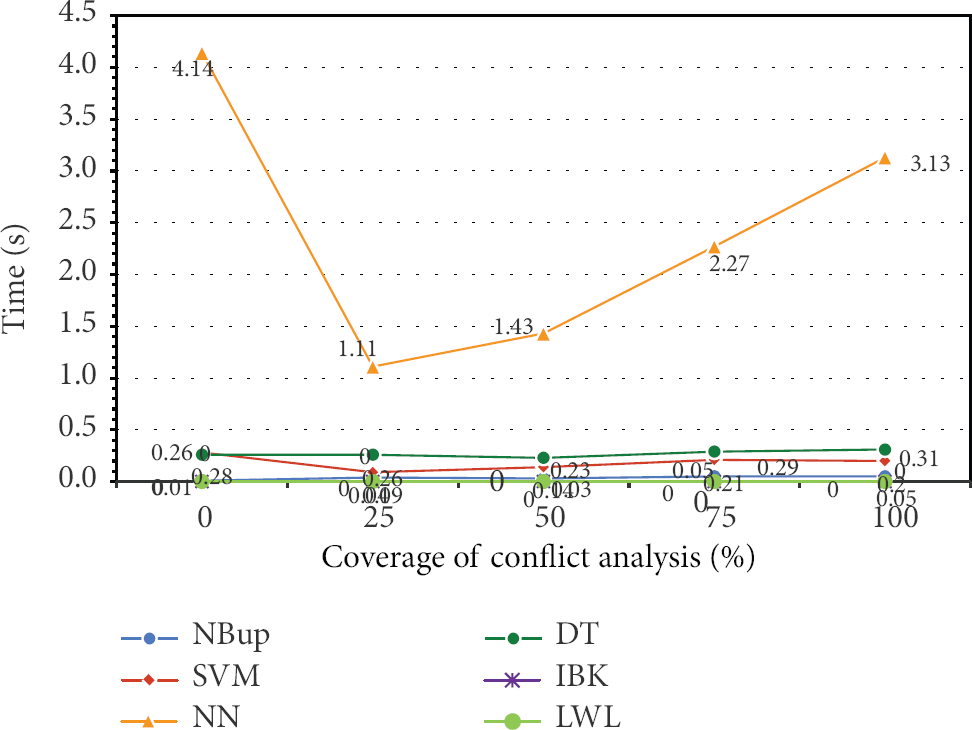
Model induction time of sonar classification by various algorithms under iDSM-CA.
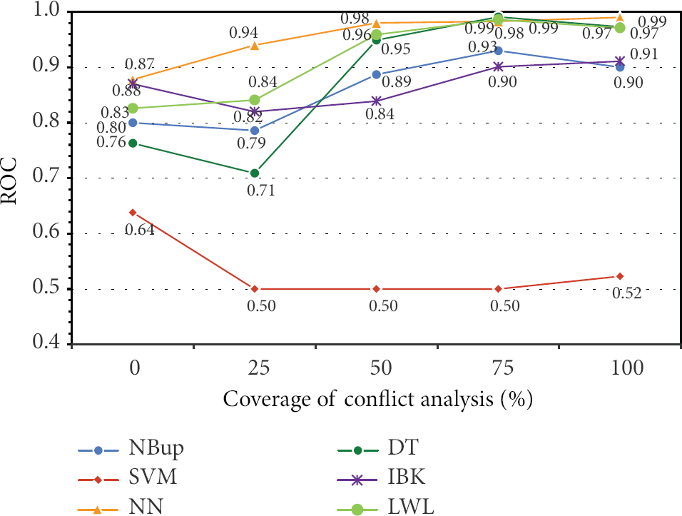
ROC of sonar classification by various algorithms under iDSM-CA.
The accuracies of the classification models differ by algorithms and by sliding window size. As we observe in Figure 6, the traditional classification algorithms generally perform worse than the incremental group of algorithms, except NN. NN in general can achieve high accuracies over various
Another important criterion in data stream mining is speed that is inferred as model induction time here, which is mainly contributed to by the time consumption required in each model update. In incremental learning, the frequency of model updates is assumed fixed; that is, each time a new instance of data streams in, the model refreshes for once in the inclusion of the new instance in model training. Figure 7 shows the average time consumption for each model update for each algorithm. All the algorithms, except NN, take approximately less than 0.4 seconds in doing a model update. NN requires the longest time when the data are not processed for noise removal at
The second part of the experiment mainly focuses on the impact of noise on the performance of sonar signal recognition by the two different classification modes (traditional versus iDSM-CA) using the six popular algorithms. In this experiment, noise is aggravated by artificially injecting perpetrated wrong target class values. The noise level is controlled by randomly fabricating certain percentage of target class values in the dataset with wrong values. As a result, the performance for all the algorithms would fall. This represents an extreme scenario where the underwater sonar is prone to heavy noise such as background inference, faulty sensors, or target of detection located nearly out of range. The range of noise manipulated in this experiment is kept within 50%. When the noise exceeds 50%, the classifiers start to mistakenly assume the wrong values in the noise as true values as majority dominates, leading to meaningless evaluation. The accuracy of each classifier in both learning modes during the noise amplification is shown from Figure 9(a) to Figure 9(f), respectively. Likewise, the charts for time consumption are from Figure 10(a) to Figure 10(e); and the charts for ROC are from Figure 11(a) to Figure 11(f). In this case, the window size for incremental learning is held fixed at 80.

(a) Accuracy of NBup under extra noise in batch and incremental learning modes. (b) Accuracy of SVM under extra noise in batch and incremental learning modes. (c) Accuracy of NN under extra noise in batch and incremental learning modes. (d) Accuracy of DT under extra noise in batch and incremental learning modes. (e) Accuracy of IBK under extra noise in batch and incremental learning modes. (f) Accuracy of LWL under extra noise in batch and incremental learning modes.

(a) Time of NBup under extra noise in batch and incremental learning modes. (b) Time of SVM under extra noise in batch and incremental learning modes. (c) Time of NN under extra noise in batch and incremental learning modes. (d) Time of DT under extra noise in batch and incremental learning modes. (e) Time of IBK under extra noise in batch and incremental learning modes. (f) Time of LWL under extra noise in batch and incremental learning modes.

(a) ROC of NBup under extra noise in batch and incremental learning modes. (b) ROC of SVM under extra noise in batch and incremental learning modes. (c) ROC of NN under extra noise in batch and incremental learning modes. (d) ROC of DT under extra noise in batch and incremental learning modes. (e) ROC of IBK under extra noise in batch and incremental learning modes. (f) ROC of LWL under extra noise in batch and incremental learning modes.
As observed from Figure 9(a) to Figure 9(f), most of the algorithms in incremental learning mode under certain noise levels outperform those in batch learning mode. For NBup, incremental mode is good when the noise level is slight; when the noise level increases, NBup of incremental mode falls behind that of batch mode in accuracy. The same is observed from SVM and NN. Except near 50% noise level that is the oblivion state where noise and true instances can no longer be distinguished, the incremental learning mode shows some slight improvement. On the other hand, algorithms in incremental learning mode like DT, IBK, and LWL show an edge in accuracy. In particular LWL, it shows superior accuracy under light and moderate noises as in Figure 9(f). To sum up, most of the algorithms under noise perform better in incremental learning mode, except NN which underperforms only at noise level equals to 50%.
When it comes to time consumption, generally the algorithms in batch learning mode take far longer time than the same in incremental learning mode. For instance, LWL takes almost zero time in both incremental and batch learning modes, regardless of noise level being inflicted in the data stream. The differences in time consumptions are very obvious in NBup (noise levels at 10% and 20%) and in SVM and NN. It is observed that these classical classification algorithms speed up in time when put into incremental mode, being trained with only a portion of data at a time, yet attaining a reasonable level of accuracy. NBup however is quite unstable as shown in Figure 10(a) as the algorithm is mainly a prior probability based, where confusion arises relatively more easily.
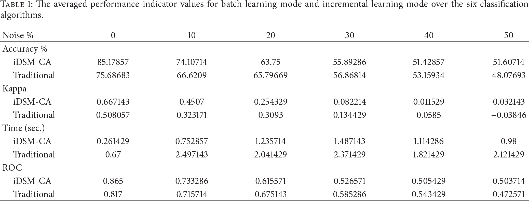
For ROC which depicts the extent of precision and sensitivity of the classifiers, NBup, SVM, and NN in batch learning mode largely demonstrate consistent performance across various levels of noise. In contrast, these algorithms in incremental learning mode run somewhat short of ROC performance, as there would be many false alarms and misses from the targets. This is mainly due to the fact that incremental learning relies on a portion of data to be used for training at a time in maintaining the prediction power of the classifiers. Batch learning has the luxury of digesting through the whole set of data in model induction. Nevertheless, DT and LWL, when operating under incremental learning mode, prevail in terms of ROC in most noise levels. As a remark, lightweight algorithms seem to perform fast and exhibit advantages in performance (accuracy and ROC) in the incremental mode (iDSM-CA). Over all the algorithms, the performance characters are averaged for the sake of comparing the tasks of sonar signal recognition by batch learning mode and incremental learning mode. Table 1 shows the averaged results at a glance. The accuracy of incremental learning in average surpasses that of batch learning in light noises, but it quickly descends when the noises worsen, due to model induction with only partial data. The same is observed with respect to ROC and Kappa statistics that usually are used for signifying the reliability and generalization of the datasets. Incremental learning is indeed faster than batch learning.
The averaged performance indicator values for batch learning mode and incremental learning mode over the six classification algorithms.
5. Conclusion
Accurate recognition of sonar signal is known to be a challenging problem though it has a significant contribution in military applications. One major factor in deteriorating the accuracy is noise in the ambient underwater environment. Noise causes confusion in the construction of classification models. Noisy data or instance in the training dataset is regarded as those contradicting ones that do not agree with the majority of the data; this disagreement leads to erroneous rules in classification models and disrupts homogenous metaknowledge or statistical patterns by distorting the training patterns. Other authors refer to noise as outliers, misclassified instances, or misfits, all of which are data types the removal of which will improve the accuracy of the classification model. Though this research topic has been studied for over two decades, techniques previously proposed for removing such noise assume batch operations requiring the full dataset to be used in noise detection.
In this paper, we described a novel preprocessing strategy called iDSM-CA that stands for incremental data stream mining with conflict analysis. The main advantage of the iDSM-CA lies in its lightweight window sliding mechanism designed for mining moving data streams. The iDSM-CA model is extremely simple to use in comparison with other more complex techniques such as those outlined in Section 2. Our experiment validates its benefits in terms of its high speed and its efficacy in providing a noise-resilient streamlined training dataset for incremental learning, using empirical sonar data in distinguishing metal or rock objects. It is shown that iDSM-CA is effective and efficient in mining stream data by experiments. Analyzing data stream on the fly is important in many big data type of applications such as data mining sport activities [19] and data feeds from social media [20] in real time, just to name a few.
Footnotes
Conflict of Interests
The authors declare that there is no conflict of interests regarding the publication of this paper.
Acknowledgments
The authors are thankful for the financial support from the Research Grant “Adaptive OVFDT with Incremental Pruning and ROC Corrective Learning for Data Stream Mining,” Grant no. MYRG073(Y3-L2)-FST12-FCC, offered by the University of Macau, FST, and RDAO.