Constraint Analysis and Redundancy of Planar Closed Loop Double Chain Linkages

Abstract

This paper studies the kinematics of planar closed double chain linkages using the natural coordinate method. Different constraints including the rigid bar, pin joint, generalized angulated element (GAE) joint, and the boundary conditions of linkages were firstly used to form the system constraint equations. Then the degree of freedom of the linkages was calculated from the dimension of null space of the Jacobian matrix, which is the derivative of the constraint equations with respect to time. Furthermore, the redundant constraints can also be given by this method. Many types of planar linkages, such as the Hoberman linkage, Types I and II GAEs, nonintersecting GAEs, and linkages with the loop parallelogram condition, were investigated in this paper. It is found that when three boundary conditions are added to the system, the global motion of the system is lost. The results show that these linkages have only one degree of freedom. Moreover, the last two GAE constraints of the numerical examples given in this paper are redundant.

1. Introduction

Kempe reported that an assembly of two planar 4R linkages, which are connected with four additional revolute joints, can be moved under certain circumstances [1]. From a different angle, this linkage can also be regarded as a closed loop double chain linkage consisting of several pairs of scissor like elements. Naturally it becomes interesting to see whether the system is movable or not when it is constructed by pairs of scissor like elements.

Generally, the parallel scissor like element is the most commonly used form for deployable or foldable structures in engineering [2–4]. A parallel scissor like element in two-dimensional forms, which is shown in Figure 1(a), can be made from two straight rods connected by scissor hinges, or revolute joints at the common middle point. The axis of the revolute joint is perpendicular to the plane of the structure [5–7]. The element has one degree of freedom and can be folded and deployed freely. When two or more of such elements are added to form a system, the number of degrees of freedom will not change. However, the closed loop system consisting of parallel scissor like elements alone cannot move.

Figure 1:

Scissor like elements.

In the early 1990s, Hoberman [8, 9] invented and patented a method for constructing loop assemblies formed by the modified scissor like element, which consists of a pair of identical angulated rods connected by a revolute joint as shown in Figure 1(b). Therefore, the unit is also called angulated scissor like element or Hoberman's unit. You and Pellegrino [10] noted that the unit subtends a constant angle as their rods rotate while maintaining the end pivots on parallel lines. Thus it can form a closed loop mechanism, which is called Hoberman's linkage as shown in Figure 2. They also proposed two types of generalized angulated elements (GAEs), which subtend a constant angle during folding but afford much greater freedom of shapes than Hoberman's unit. The triangles of the two angulated rods of Type I GAE are isosceles triangles; that is, AE = DE and BE = CE, as shown in Figure 3. The triangles of the two angulated rods of Type II GAE are similar triangles to AE/BE = DE/CE and ∠AEB = ∠DEC, which are shown in Figure 4.

Figure 2:

Hoberman's linkages.

Figure 3:

Type I GAE formed by angulated rods.

Figure 4:

Type II GAE formed by angulated rods.

On the other side, Wohlart [11] has proposed a new double chain linkage. Unlike the elements in the above studies given by You and Pellegrino, the scissor like element for this closed loop linkage is a nonintersecting pair, as shown in Figure 5. Thus the GAE can be divided into two kinds: intersecting pairs (Type I GAE and Type II GAE) and nonintersecting pairs. As for a single pair of GAEs, an intersecting pair can be obtained by transforming a nonintersecting pair through a large relative rotation. They also proposed that the nonintersecting pairs can form a closed loop double chain under the loop parallelogram condition; that is, in the system each set of four neighboring revolute joints forms a parallelogram. Then Mao et al. [12] have proved the double chain can be formed by intersecting and nonintersecting pairs as well as a mixture of both pairs by the loop parallelogram condition.

Figure 5:

Nonintersecting pairs of angulated scissor elements.

Typical linkages have large number of links and joints. For the articulated linkages with double or multiple loops, the degree of freedom can be obtained by Maxwell's rule [13] or the equilibrium matrix method [14, 15]. However, these methods cannot be suited for linkages with scissor like elements. The Grübler-Kutzback criteria are often used for the mechanism with arbitrary types of joints. However, it usually gives numbers of degrees of freedom less than one, being thus unable to give a true number [6]. Dai et al. studied the mobility of a general class of foldable mechanisms using the principles of screw theory [16–21]. Zhao et al. [22] applied the screw theory to study the degree of freedom of simple planar linkage and the mechanism theory of forming the spatial deployable units utilized in flat, cylindrical, and spherical deployable structures. Moreover, they also used the same method to investigate the mobility of a foldable stair, which consists of a number of identical deployable scissor like elements which form the staircases when expanded. They pointed out that using screw theory, which is used to study the mobility of deployable structures, has many advantages compared to some classical methods. Recently, a numerical algorithm was proposed by Nagaraj et al. [23] to evaluate the degree of freedom of pantograph masts by obtaining the null space of a constraint Jacobian matrix. They also extend this method to study the static analysis of pantograph mast [24]. However, their work was only focused on the scissor like elements with straight rods. The GAEs with angulated rods are not considered in the literature. Therefore, the aim of this paper is to evaluate the degree of freedom of closed loop double chain linkages consisting of intersecting or nonintersecting pairs of GAEs using the Jacobian matrix.

2. Kinematic Modeling

Figure 6 shows a pair of general angulated scissor elements. The angulated rods 12 and 34 are connected with the revolute joint p. The angulated rod 12 can be seen as being composed of the two straight rods 1p and 2p, with a length of a and b, respectively. Similarly, the angulated rod 34 can be seen as being composed of the two straight rods 3p and 4p, with a length of c and d, respectively. The natural coordinates are used in this paper to model the GAEs. All points of interest whose positions are considered a primary unknown variable are defined as basic points. The rigid constraints of links and joint constraints are given in the natural coordinate system [23].

Figure 6:

Geometric descriptions of angulated scissor elements.

2.1. Rigid Bar Constraints

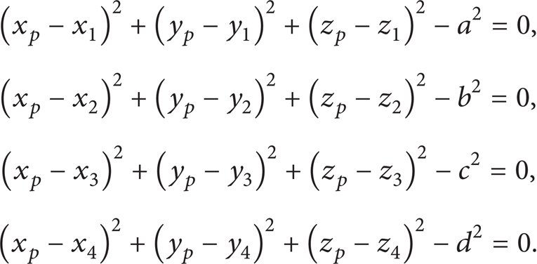
A rigid bar is used to connect the two natural coordinates i and j. Thus the distance between these two joints is a constant, which is given as

${\mathbf{X}}_{ij}^T{\mathbf{X}}_{ij}=l_{ij}^{\mathrm{2}},$

(1)

where $l_{ij}^{}$ is the length of bar ij, that is, the distance between joints i and j, Xij is the vector from joint j to joint i as ${\left[\left(x_i-x_j\right),\left(y_i-y_j\right),\left(z_i-z_j\right)\right]}^T$ , (x _i ,y _i ,z _i ), and (x _j ,y _j ,z _j ) are the natural coordinates of joints i and j, respectively.

Then from Figure 6, we can obtain the rigid bar constraints as

$\begin{array}{c}{\left(x_p-x_{\mathrm{1}}\right)}^{\mathrm{2}}+{\left(y_p-y_{\mathrm{1}}\right)}^{\mathrm{2}}+{\left(z_p-z_{\mathrm{1}}\right)}^{\mathrm{2}}-a^{\mathrm{2}}=\mathrm{0},\\ {\left(x_p-x_{\mathrm{2}}\right)}^{\mathrm{2}}+{\left(y_p-y_{\mathrm{2}}\right)}^{\mathrm{2}}+{\left(z_p-z_{\mathrm{2}}\right)}^{\mathrm{2}}-b^{\mathrm{2}}=\mathrm{0},\\ {\left(x_p-x_{\mathrm{3}}\right)}^{\mathrm{2}}+{\left(y_p-y_{\mathrm{3}}\right)}^{\mathrm{2}}+{\left(z_p-z_{\mathrm{3}}\right)}^{\mathrm{2}}-c^{\mathrm{2}}=\mathrm{0},\\ {\left(x_p-x_{\mathrm{4}}\right)}^{\mathrm{2}}+{\left(y_p-y_{\mathrm{4}}\right)}^{\mathrm{2}}+{\left(z_p-z_{\mathrm{4}}\right)}^{\mathrm{2}}-d^{\mathrm{2}}=\mathrm{0}.\end{array}$

(2)

2.2. Pin Joint Constraints

The relative motion of the joint between the connected rods is related to joint constraints. The constraints corresponding to pin joints are automatically satisfied when adjacent rods share a common point [23, 24].

2.3. GAE Constraints

As shown in Figure 6, the rods 12 and 34 are coplanar and can rotate around the revolute joints. It is assumed that the two rods are not equal and the revolute joint is not in the middle. The segments 1p and 2p of rod 12 are aligned at the revolute joint. Therefore, the cross-product of the two adjacent rod segments 1p and 2p is given by

$\left|{\mathbf{X}}_{\mathrm{1}p}\times {\mathbf{X}}_{\mathrm{2}p}\right|-ab\sin \alpha =\mathrm{0},$

(3)

where α is the angle between the two rod segments 1p and 2p. Similarly, the constraint equation for rod 34 is given by

$\left|{\mathbf{X}}_{\mathrm{3}p}\times {\mathbf{X}}_{\mathrm{4}p}\right|-cd\sin \beta =\mathrm{0},$

(4)

Where β is the angle between the two rod segments 1p and 2p.

2.4. Boundary Constraints

Boundary constraints are used to exclude the global motion of the mechanism. For example, if joint 1 is fixed as shown in Figure 6, its constraint is given as

$x_{\mathrm{1}}=y_{\mathrm{1}}=z_{\mathrm{1}}=\mathrm{0}.$

(5)

For the closed loop double chain linkage shown in Figure 2, it is a planar mechanism. Then one of the boundary constraints is

$z_{\mathrm{1}}=z_{\mathrm{2}}=z_{\mathrm{3}}=z_{\mathrm{4}}=z_p=\cdots =\mathrm{0}.$

(6)

2.5. System Constraints

The rigid bar constraints, pin joint constraints, GAE constraints, and boundary constraints of a linkage can be rewritten together as

$\begin{array}{c}{f}_j\left(x_{\mathrm{1}},x_{\mathrm{2}},\dots ,x_n,y_{\mathrm{1}},y_{\mathrm{2}},\dots ,y_n,z_{\mathrm{1}},z_{\mathrm{2}},\dots ,z_n\right)=\mathrm{0}\\ j=\mathrm{1},\mathrm{2},\dots ,m,\end{array}$

(7)

where m is the number of constraint equations and n is the number of joints of the linkages. The derivative of the system constraint equations with respect to time leads to the Jacobian matrix, given by

$\left[\mathbf{B}\right]\dot{\mathbf{X}}=\mathrm{0}.$

(8)

Equation (8) is a homogeneous equation. Thus if the dimension of the null space of B is more than one, a nonnull vector of $\dot{\mathbf{X}}$ is obtained. The existence of the null space implies that the linkages possess one degree of freedom along the corresponding $\dot{\mathbf{X}}$ [23]. Therefore, the degree of freedom of the linkage is the dimension of the null space of B, which can be obtained numerically or symbolically. However, the closed-form solution with the symbolic method can only be used for simple linkages. Hence the numerical method is used to calculate the degree of freedom of the linkage at a chosen configuration.

3. Numerical Algorithm

If the planar closed loop double loop chain linkage has n joints, the number of natural coordinates is 2n. In this study, the pin joints are used to connect the adjacent angulated scissor like elements. The main steps in the numerical algorithm are as follows.

1. Establish all the rigid bar constraint equations and compute the dimension of null space of B.

2. Add one GAE constraint at each step and evaluate the dimension of null space of B. If the dimension of null space of B does not decrease when a GAE constraint is added, this constraint is redundant.

3. Add one boundary constraint at each step and evaluate the dimension of null space of B. If the dimension of null space of B does not decrease after adding a boundary constraint, this constraint is redundant.

4. After adding all the constraints, the final dimension of the null space of B is the degree of freedom of the linkage.

4. Numerical Examples

In this section, the results obtained using the numerical algorithm given in Section 3 for exemplary planar closed loop double chain linkages are presented. In addition to the degree of freedom of the system, the redundant constraints are also given.

4.1. Hoberman's Linkage

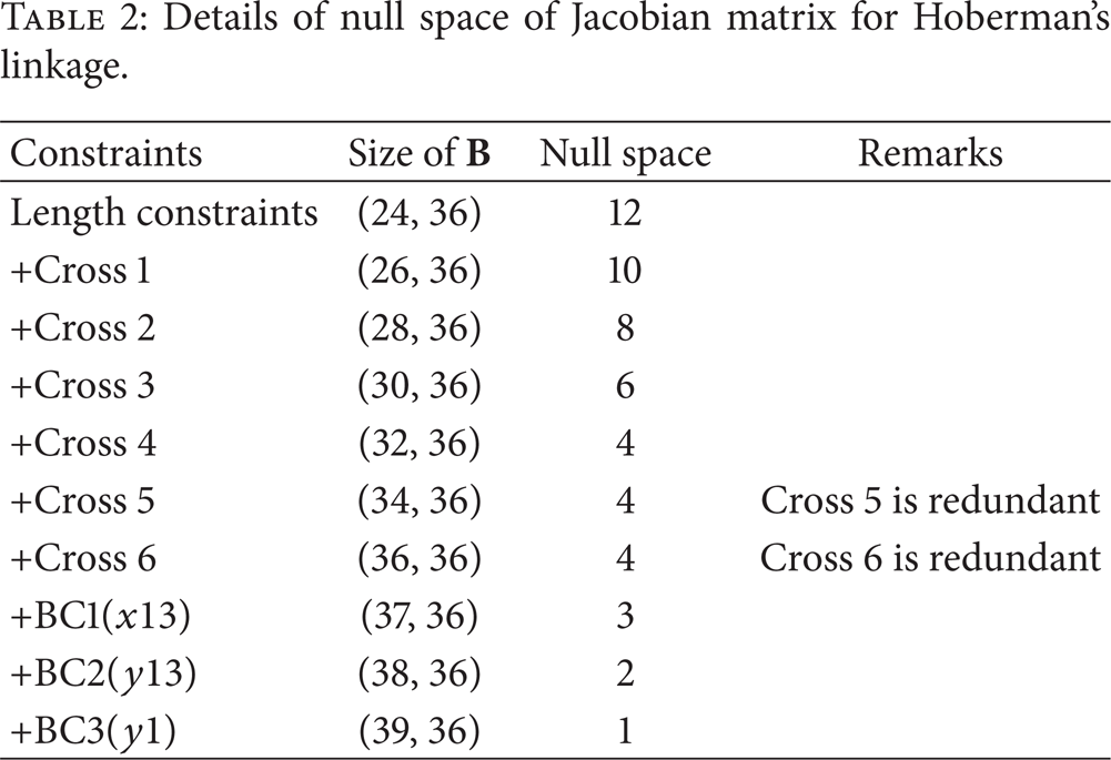
Figure 7 shows a Hoberman linkage with six Hoberman units. Every Hoberman unit has four rigid bar constraints and a GAE constraint. The linkage is fixed at joint 13. The additional boundary condition at point 1 is imposed in the oy direction. The natural coordinates of all joints are given in Table 1. System constraint equations are given in (9). The results of null space are presented in Table 2. It can be seen from this table that the null space reduces by two by adding each constraint of the first four GAEs. The null space does not change for constraints after imposing the last two GAEs. Therefore, two of the six GAE constraints are redundant. The final dimension of null space for the linkage is 1, and thus the degree of freedom of Hoberman's linkage is 1.

$\begin{array}{c}\text{Length}\hspace{0.17em}\hspace{0.17em}\text{constraints:}\\ \hspace{1em}\hspace{1em}{\left(x_{\mathrm{1}}-x_{\mathrm{13}}\right)}^{\mathrm{2}}+{\left(y_{\mathrm{1}}-y_{\mathrm{13}}\right)}^{\mathrm{2}}-\mathrm{2}=\mathrm{0},\\ \hspace{1em}\hspace{1em}{\left(x_{\mathrm{2}}-x_{\mathrm{13}}\right)}^{\mathrm{2}}+{\left(y_{\mathrm{2}}-y_{\mathrm{13}}\right)}^{\mathrm{2}}-\mathrm{2}=\mathrm{0},\\ \hspace{1em}\hspace{1em}{\left(x_{\mathrm{3}}-x_{\mathrm{13}}\right)}^{\mathrm{2}}+{\left(y_{\mathrm{3}}-y_{\mathrm{13}}\right)}^{\mathrm{2}}-\mathrm{2}=\mathrm{0},\\ \hspace{1em}\hspace{1em}{\left(x_{\mathrm{4}}-x_{\mathrm{13}}\right)}^{\mathrm{2}}+{\left(y_{\mathrm{4}}-y_{\mathrm{13}}\right)}^{\mathrm{2}}-\mathrm{2}=\mathrm{0},\\ \hspace{1em}\hspace{1em}{\left(x_{\mathrm{3}}-x_{\mathrm{14}}\right)}^{\mathrm{2}}+{\left(y_{\mathrm{3}}-y_{\mathrm{14}}\right)}^{\mathrm{2}}-\mathrm{2}=\mathrm{0},\\ \hspace{1em}\hspace{1em}{\left(x_{\mathrm{4}}-x_{\mathrm{14}}\right)}^{\mathrm{2}}+{\left(y_{\mathrm{4}}-y_{\mathrm{14}}\right)}^{\mathrm{2}}-\mathrm{2}=\mathrm{0},\\ \hspace{1em}\hspace{1em}{\left(x_{\mathrm{5}}-x_{\mathrm{14}}\right)}^{\mathrm{2}}+{\left(y_{\mathrm{5}}-y_{\mathrm{14}}\right)}^{\mathrm{2}}-\mathrm{2}=\mathrm{0},\\ \hspace{1em}\hspace{1em}{\left(x_{\mathrm{6}}-x_{\mathrm{14}}\right)}^{\mathrm{2}}+{\left(y_{\mathrm{6}}-y_{\mathrm{14}}\right)}^{\mathrm{2}}-\mathrm{2}=\mathrm{0},\\ \hspace{1em}\hspace{1em}{\left(x_{\mathrm{5}}-x_{\mathrm{15}}\right)}^{\mathrm{2}}+{\left(y_{\mathrm{5}}-y_{\mathrm{15}}\right)}^{\mathrm{2}}-\mathrm{2}=\mathrm{0},\\ \hspace{1em}\hspace{1em}{\left(x_{\mathrm{6}}-x_{\mathrm{15}}\right)}^{\mathrm{2}}+{\left(y_{\mathrm{6}}-y_{\mathrm{15}}\right)}^{\mathrm{2}}-\mathrm{2}=\mathrm{0},\\ \hspace{1em}\hspace{1em}{\left(x_{\mathrm{7}}-x_{\mathrm{15}}\right)}^{\mathrm{2}}+{\left(y_{\mathrm{7}}-y_{\mathrm{15}}\right)}^{\mathrm{2}}-\mathrm{2}=\mathrm{0},\\ \hspace{1em}\hspace{1em}{\left(x_{\mathrm{8}}-x_{\mathrm{15}}\right)}^{\mathrm{2}}+{\left(y_{\mathrm{8}}-y_{\mathrm{15}}\right)}^{\mathrm{2}}-\mathrm{2}=\mathrm{0},\\ \hspace{1em}\hspace{1em}{\left(x_{\mathrm{7}}-x_{\mathrm{16}}\right)}^{\mathrm{2}}+{\left(y_{\mathrm{7}}-y_{\mathrm{16}}\right)}^{\mathrm{2}}-\mathrm{2}=\mathrm{0},\\ \hspace{1em}\hspace{1em}{\left(x_{\mathrm{8}}-x_{\mathrm{16}}\right)}^{\mathrm{2}}+{\left(y_{\mathrm{8}}-y_{\mathrm{16}}\right)}^{\mathrm{2}}-\mathrm{2}=\mathrm{0},\\ \hspace{1em}\hspace{1em}{\left(x_{\mathrm{9}}-x_{\mathrm{16}}\right)}^{\mathrm{2}}+{\left(y_{\mathrm{9}}-y_{\mathrm{16}}\right)}^{\mathrm{2}}-\mathrm{2}=\mathrm{0},\\ \hspace{1em}\hspace{1em}{\left(x_{\mathrm{10}}-x_{\mathrm{16}}\right)}^{\mathrm{2}}+{\left(y_{\mathrm{10}}-y_{\mathrm{16}}\right)}^{\mathrm{2}}-\mathrm{2}=\mathrm{0},\\ \hspace{1em}\hspace{1em}{\left(x_{\mathrm{9}}-x_{\mathrm{17}}\right)}^{\mathrm{2}}+{\left(y_{\mathrm{9}}-y_{\mathrm{17}}\right)}^{\mathrm{2}}-\mathrm{2}=\mathrm{0},\\ \hspace{1em}\hspace{1em}{\left(x_{\mathrm{10}}-x_{\mathrm{17}}\right)}^{\mathrm{2}}+{\left(y_{\mathrm{10}}-y_{\mathrm{17}}\right)}^{\mathrm{2}}-\mathrm{2}=\mathrm{0},\\ \hspace{1em}\hspace{1em}{\left(x_{\mathrm{11}}-x_{\mathrm{17}}\right)}^{\mathrm{2}}+{\left(y_{\mathrm{11}}-y_{\mathrm{17}}\right)}^{\mathrm{2}}-\mathrm{2}=\mathrm{0},\\ \hspace{1em}\hspace{1em}{\left(x_{\mathrm{12}}-x_{\mathrm{17}}\right)}^{\mathrm{2}}+{\left(y_{\mathrm{12}}-y_{\mathrm{17}}\right)}^{\mathrm{2}}-\mathrm{2}=\mathrm{0},\\ \hspace{1em}\hspace{1em}{\left(x_{\mathrm{11}}-x_{\mathrm{18}}\right)}^{\mathrm{2}}+{\left(y_{\mathrm{11}}-y_{\mathrm{18}}\right)}^{\mathrm{2}}-\mathrm{2}=\mathrm{0},\\ \hspace{1em}\hspace{1em}{\left(x_{\mathrm{12}}-x_{\mathrm{18}}\right)}^{\mathrm{2}}+{\left(y_{\mathrm{12}}-y_{\mathrm{18}}\right)}^{\mathrm{2}}-\mathrm{2}=\mathrm{0},\\ \hspace{1em}\hspace{1em}{\left(x_{\mathrm{1}}-x_{\mathrm{18}}\right)}^{\mathrm{2}}+{\left(y_{\mathrm{1}}-y_{\mathrm{18}}\right)}^{\mathrm{2}}-\mathrm{2}=\mathrm{0},\\ \hspace{1em}\hspace{1em}{\left(x_{\mathrm{1}}-x_{\mathrm{18}}\right)}^{\mathrm{2}}+{\left(y_{\mathrm{1}}-y_{\mathrm{18}}\right)}^{\mathrm{2}}-\mathrm{2}=\mathrm{0}.\\ \text{Cross}\hspace{0.17em}\hspace{0.17em}\mathrm{1}\text{:}\\ \hspace{1em}\left|\left(x_{\mathrm{13}}-x_{\mathrm{1}}\right)\left(y_{\mathrm{4}}-y_{\mathrm{13}}\right)-\left(x_{\mathrm{4}}-x_{\mathrm{13}}\right)\left(y_{\mathrm{13}}-y_{\mathrm{1}}\right)\right|-\sqrt{\mathrm{3}}=\mathrm{0},\\ \hspace{1em}\left|\left(x_{\mathrm{13}}-x_{\mathrm{3}}\right)\left(y_{\mathrm{2}}-y_{\mathrm{13}}\right)-\left(x_{\mathrm{2}}-x_{\mathrm{13}}\right)\left(y_{\mathrm{13}}-y_{\mathrm{3}}\right)\right|-\sqrt{\mathrm{3}}=\mathrm{0}.\\ \text{Cross}\hspace{0.17em}\hspace{0.17em}\mathrm{2}\text{:}\\ \hspace{1em}\left|\left(x_{\mathrm{14}}-x_{\mathrm{3}}\right)\left(y_{\mathrm{6}}-y_{\mathrm{14}}\right)-\left(x_{\mathrm{6}}-x_{\mathrm{14}}\right)\left(y_{\mathrm{14}}-y_{\mathrm{3}}\right)\right|-\sqrt{\mathrm{3}}=\mathrm{0},\\ \hspace{1em}\left|\left(x_{\mathrm{14}}-x_{\mathrm{5}}\right)\left(y_{\mathrm{4}}-y_{\mathrm{14}}\right)-\left(x_{\mathrm{4}}-x_{\mathrm{14}}\right)\left(y_{\mathrm{14}}-y_{\mathrm{5}}\right)\right|-\sqrt{\mathrm{3}}=\mathrm{0}.\\ \text{Cross}\hspace{0.17em}\hspace{0.17em}\mathrm{3}\text{:}\\ \hspace{1em}\left|\left(x_{\mathrm{15}}-x_{\mathrm{5}}\right)\left(y_{\mathrm{8}}-y_{\mathrm{15}}\right)-\left(x_{\mathrm{8}}-x_{\mathrm{15}}\right)\left(y_{\mathrm{15}}-y_{\mathrm{5}}\right)\right|-\sqrt{\mathrm{3}}=\mathrm{0},\\ \hspace{1em}\left|\left(x_{\mathrm{15}}-x_{\mathrm{7}}\right)\left(y_{\mathrm{6}}-y_{\mathrm{15}}\right)-\left(x_{\mathrm{6}}-x_{\mathrm{15}}\right)\left(y_{\mathrm{15}}-y_{\mathrm{7}}\right)\right|-\sqrt{\mathrm{3}}=\mathrm{0}.\\ \text{Cross}\hspace{0.17em}\hspace{0.17em}\mathrm{4}\text{:}\\ \hspace{1em}\left|\left(x_{\mathrm{16}}-x_{\mathrm{7}}\right)\left(y_{\mathrm{10}}-y_{\mathrm{16}}\right)-\left(x_{\mathrm{10}}-x_{\mathrm{16}}\right)\left(y_{\mathrm{16}}-y_{\mathrm{7}}\right)\right|-\sqrt{\mathrm{3}}=\mathrm{0},\\ \hspace{1em}\left|\left(x_{\mathrm{16}}-x_{\mathrm{9}}\right)\left(y_{\mathrm{8}}-y_{\mathrm{16}}\right)-\left(x_{\mathrm{8}}-x_{\mathrm{16}}\right)\left(y_{\mathrm{16}}-y_{\mathrm{9}}\right)\right|-\sqrt{\mathrm{3}}=\mathrm{0}.\\ \text{Cross}\hspace{0.17em}\hspace{0.17em}\mathrm{5}\text{:}\\ \hspace{1em}\left|\left(x_{\mathrm{17}}-x_{\mathrm{9}}\right)\left(y_{\mathrm{12}}-y_{\mathrm{17}}\right)-\left(x_{\mathrm{12}}-x_{\mathrm{17}}\right)\left(y_{\mathrm{17}}-y_{\mathrm{9}}\right)\right|-\sqrt{\mathrm{3}}=\mathrm{0},\\ \hspace{1em}\left|\left(x_{\mathrm{17}}-x_{\mathrm{11}}\right)\left(y_{\mathrm{10}}-y_{\mathrm{17}}\right)-\left(x_{\mathrm{10}}-x_{\mathrm{17}}\right)\left(y_{\mathrm{17}}-y_{\mathrm{11}}\right)\right|-\sqrt{\mathrm{3}}=\mathrm{0}.\\ \text{Cross}\hspace{0.17em}\hspace{0.17em}\mathrm{6}\text{:}\\ \hspace{1em}\left|\left(x_{\mathrm{18}}-x_{\mathrm{11}}\right)\left(y_{\mathrm{2}}-y_{\mathrm{18}}\right)-\left(x_{\mathrm{2}}-x_{\mathrm{18}}\right)\left(y_{\mathrm{18}}-y_{\mathrm{11}}\right)\right|-\sqrt{\mathrm{3}}=\mathrm{0},\\ \hspace{1em}\left|\left(x_{\mathrm{18}}-x_{\mathrm{1}}\right)\left(y_{\mathrm{12}}-y_{\mathrm{18}}\right)-\left(x_{\mathrm{12}}-x_{\mathrm{18}}\right)\left(y_{\mathrm{18}}-y_{\mathrm{1}}\right)\right|-\sqrt{\mathrm{3}}=\mathrm{0}.\\ \text{Boundary}\hspace{0.17em}\hspace{0.17em}\text{condition:}\\ \hspace{1em}\hspace{1em}\hspace{1em}\hspace{1em}\hspace{1em}\hspace{1em}\hspace{1em}\hspace{1em}{x}_{\mathrm{13}}=-\mathrm{1.7321},\\ \hspace{1em}\hspace{1em}\hspace{1em}\hspace{1em}\hspace{1em}\hspace{1em}\hspace{1em}\hspace{1em}{y}_{\mathrm{13}}=\mathrm{1.0000},\hspace{1em}\hspace{1em}{y}_{\mathrm{1}}=\mathrm{0.6340}.\end{array}$

(9)

Table 1:

Natural coordinates of Hoberman's linkage.

Joint number	x (m)	y (m)
Joint 1	−0.3660	0.6340
Joint 2	−1.3660	2.3660
Joint 3	−0.7321	0
Joint 4	−2.7321	0
Joint 5	−0.3660	−0.6340
Joint 6	−1.3660	−2.3660
Joint 7	0.3660	−0.6340
Joint 8	1.3660	−2.3660
Joint 9	0.7321	0
Joint 10	2.7321	0
Joint 11	0.3660	0.6340
Joint 12	1.3660	2.3660
Joint 13	−1.7321	1.0000
Joint 14	−1.7321	−1.0000
Joint 15	0	−2.0000
Joint 16	1.7321	−1.0000
Joint 17	1.7321	1.0000
Joint 18	0	2.0000

Table 2:

Details of null space of Jacobian matrix for Hoberman's linkage.

Constraints	Size of B	Null space	Remarks
Length constraints	(24, 36)	12
+ Cross 1	(26, 36)	10
+ Cross 2	(28, 36)	8
+ Cross 3	(30, 36)	6
+ Cross 4	(32, 36)	4
+ Cross 5	(34, 36)	4	Cross 5 is redundant
+ Cross 6	(36, 36)	4	Cross 6 is redundant
+ BC1(x13)	(37, 36)	3
+ BC2(y13)	(38, 36)	2
+ BC3(y1)	(39, 36)	1

Figure 7:

Hoberman's linkage.

4.2. Linkages of Type I GAEs

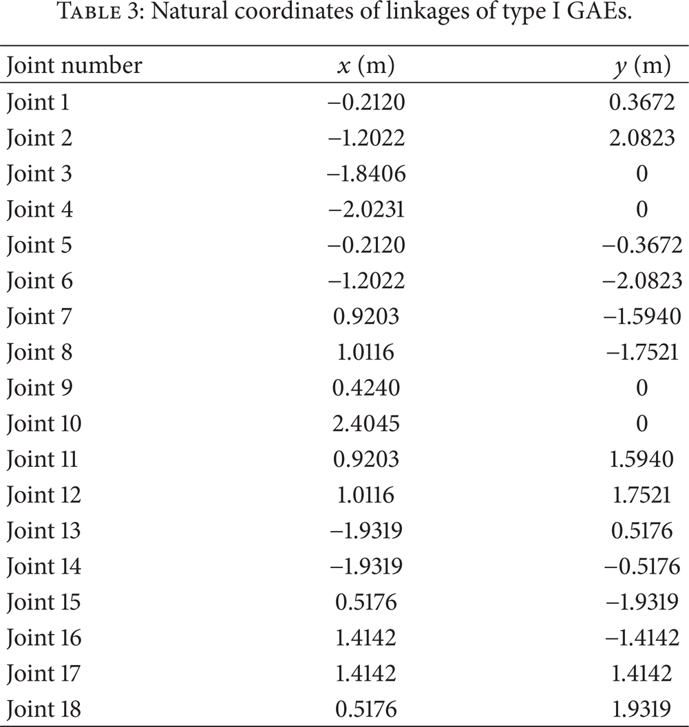
Figure 8 shows a linkage with six Type I GAEs. Every Type I GAE has four rigid bar constraints and a GAE constraint. The linkage is also fixed at joint 13. The additional boundary condition at point 1 is applied in the oy direction. The natural coordinates of all joints are given in Table 3. The results of null space are presented in Table 4. It is observed from this table that two of the six GAE constraints are redundant. The presence of three boundary conditions had excluded the global motion of the system. The final dimension of null space for the linkage is 1.

Table 3:

Natural coordinates of linkages of type I GAEs.

Joint number	x (m)	y (m)
Joint 1	−0.2120	0.3672
Joint 2	−1.2022	2.0823
Joint 3	−1.8406	0
Joint 4	−2.0231	0
Joint 5	−0.2120	−0.3672
Joint 6	−1.2022	−2.0823
Joint 7	0.9203	−1.5940
Joint 8	1.0116	−1.7521
Joint 9	0.4240	0
Joint 10	2.4045	0
Joint 11	0.9203	1.5940
Joint 12	1.0116	1.7521
Joint 13	−1.9319	0.5176
Joint 14	−1.9319	−0.5176
Joint 15	0.5176	−1.9319
Joint 16	1.4142	−1.4142
Joint 17	1.4142	1.4142
Joint 18	0.5176	1.9319

Table 4:

Details of null space of Jacobian matrix for linkages of type I GAEs.

Constraints	Size of B	Null space	Remarks
Length constraints	(24, 36)	12
+ Cross 1	(26, 36)	10
+ Cross 2	(28, 36)	8
+ Cross 3	(30, 36)	6
+ Cross 4	(32, 36)	4
+ Cross 5	(34, 36)	4	Cross 5 is redundant
+ Cross 6	(36, 36)	4	Cross 6 is redundant
+ BC1(x13)	(37, 36)	3
+ BC2(y13)	(38, 36)	2
+ BC3(y1)	(39, 36)	1

Figure 8:

Linkage of Type I GAEs.

4.3. Linkages of Type II GAEs

Figure 9 shows a linkage with six Type II GAEs. Every Type II GAE has four rigid bar constraints and a GAE constraint. The linkage is also fixed at joint 13. The additional boundary condition at point 1 is in the oy direction. The natural coordinates of all joints are given in Table 5. The results of null space are presented in Table 6. It is observed from this table that two of the six GAE constraints are redundant. The three boundary conditions exclude the global motion of the system. The final dimension of null space for the linkage is 1.

Table 5:

Natural coordinates of linkages of type II GAEs.

Joint number	x (m)	y (m)
Joint 1	−0.2989	0.5176
Joint 2	−1.4142	2.4495
Joint 3	−1.4142	0
Joint 4	−2.2307	0
Joint 5	−0.2989	−0.5176
Joint 6	−1.4142	−2.4495
Joint 7	0.7071	−1.2247
Joint 8	1.1154	−1.9319
Joint 9	0.5977	0
Joint 10	2.8284	0
Joint 11	0.7071	1.2247
Joint 12	1.1154	1.9319
Joint 13	−1.9319	0.5176
Joint 14	−1.9319	−0.5176
Joint 15	0.5176	−1.9319
Joint 16	1.4142	−1.4142
Joint 17	1.4142	1.4142
Joint 18	0.5176	1.9319

Table 6:

Details of null space of Jacobian matrix for linkages of type II GAEs.

Constraints	Size of B	Null space	Remarks
Length constraints	(24, 36)	12
+ Cross 1	(26, 36)	10
+ Cross 2	(28, 36)	8
+ Cross 3	(30, 36)	6
+ Cross 4	(32, 36)	4
+ Cross 5	(34, 36)	4	Cross 5 is redundant
+ Cross 6	(36, 36)	4	Cross 6 is redundant
+ BC1(x13)	(37, 36)	3
+ BC2(y13)	(38, 36)	2
+ BC3(y1)	(39, 36)	1

Figure 9:

Linkage of Type II GAEs.

4.4. Linkages of Nonintersecting GAEs

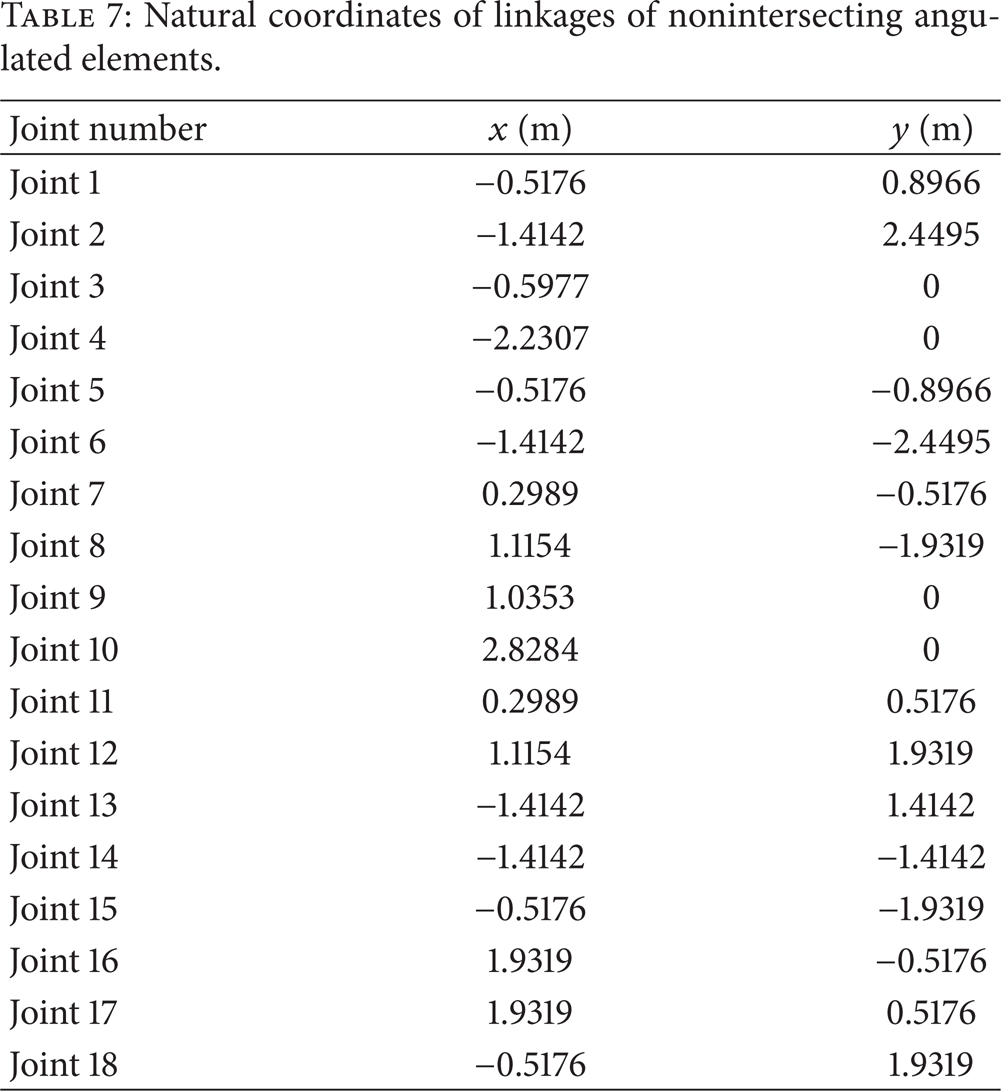
Figure 10 shows a linkage with six nonintersecting GAEs. Every nonintersecting GAE has four rigid bar constraints and a GAE constraint. The linkage is also fixed at joint 13. The additional boundary condition at point 1 is in the oy direction. The natural coordinates of all joints are given in Table 7. The results of null space are presented in Table 8. It is observed from this table that two of the six GAE constraints are redundant. The three boundary conditions exclude the global motion of the system. The final dimension of null space for the linkage is 1.

Table 7:

Natural coordinates of linkages of nonintersecting angulated elements.

Joint number	x (m)	y (m)
Joint 1	−0.5176	0.8966
Joint 2	−1.4142	2.4495
Joint 3	−0.5977	0
Joint 4	−2.2307	0
Joint 5	−0.5176	−0.8966
Joint 6	−1.4142	−2.4495
Joint 7	0.2989	−0.5176
Joint 8	1.1154	−1.9319
Joint 9	1.0353	0
Joint 10	2.8284	0
Joint 11	0.2989	0.5176
Joint 12	1.1154	1.9319
Joint 13	−1.4142	1.4142
Joint 14	−1.4142	−1.4142
Joint 15	−0.5176	−1.9319
Joint 16	1.9319	−0.5176
Joint 17	1.9319	0.5176
Joint 18	−0.5176	1.9319

Table 8:

Details of null space of Jacobian matrix for linkages of nonintersecting angulated elements.

Constraints	Size of B	Null space	Remarks
Length constraints	(24, 36)	12
+ Cross 1	(26, 36)	10
+ Cross 2	(28, 36)	8
+ Cross 3	(30, 36)	6
+ Cross 4	(32, 36)	4
+ Cross 5	(34, 36)	4	Cross 5 is redundant
+ Cross 6	(36, 36)	4	Cross 6 is redundant
+ BC1(x13)	(37, 36)	3
+ BC2(y13)	(38, 36)	2
+ BC3(y1)	(39, 36)	1

Figure 10:

Linkage of nonintersecting angulated elements.

4.5. Linkages with the Loop Parallelogram Condition

Figure 11 shows a linkage with four angulated elements by the loop parallelogram condition. Each angulated element has four rigid bar constraints and a GAE constraint. The linkage is also fixed at joint 9. The additional boundary condition at point 1 is applied in the oy direction. The natural coordinates of all joints are given in Table 9. The results of null space are presented in Table 10. It can be seen from this table that the null space is reduced by two by imposing every constraint of the first two angulated elements. The null space does not change for constraints of the last two angulated elements. Therefore, two of the four angulated elements constraints are redundant. The final dimension of null space for the linkage is 1, and thus the degree of freedom of the linkage is 1.

Table 9:

Natural coordinates of linkages with the loop parallelogram condition.

Joint number	x (m)	y (m)
Joint 1	0.3922	0.1904
Joint 2	0.2032	0.4519
Joint 3	0.4104	−0.1219
Joint 4	0.0869	−0.3906
Joint 5	0.7075	−0.0554
Joint 6	1.0264	−0.4632
Joint 7	0.6716	0.2391
Joint 8	1.1605	0.3971
Joint 9	0	0
Joint 10	0.4973	−0.5125
Joint 11	1.2366	−0.0061
Joint 12	0.5954	0.6423

Table 10:

Details of null space of Jacobian matrix for linkages with the loop parallelogram condition.

Constraints	Size of B	Null space	Remarks
Length constraints	(16, 24)	8
+ Cross 1	(18, 24)	6
+ Cross 2	(20, 24)	4
+ Cross 3	(22, 24)	4	Cross 3 is redundant
+ Cross 4	(24, 24)	4	Cross 4 is redundant
+ BC1(x9)	(25, 24)	3
+ BC2(y9)	(26, 24)	2
+ BC3(y1)	(27, 24)	1

Figure 11:

Linkages with the loop parallelogram condition.

5. Conclusions

In this paper, the kinematics of planar closed double chain linkages were studied using the natural coordinate method. The rigid bar constraints, pin joint constraints, GAE constraints, and boundary constraints of linkages firstly formed the system constraint equations. Then the Jacobian matrix was obtained by the derivative of the constraint equations with respect to time. The degree of freedom of the linkages was calculated from the dimension of null space of the Jacobian matrix. Furthermore, an algorithm was given to obtain the details of the redundant constraints. Hoberman's linkage, linkage with Type I GAEs, linkage with Type II GAEs, linkages with nonintersecting GAEs, and linkages with the loop parallelogram condition were investigated in this paper. When three boundary conditions are added to the system, the global motion of the system was excluded. The results show that the degree of freedom of these linkages is one. Moreover, the last two GAE constraints of the numerical examples given in this paper are redundant.

It should be noted that linkages with a more general angulated scissor element containing intermediate parallelograms, as reported by You and Pellegrino [10], can also be investigated with the help of this theory. Moreover, the method given in this paper can be used to find some new planar closed loop linkage. However, if the linkages have many singular kinematic paths in some special configurations [25], the method given in this paper cannot give the true degree of freedom of the system, and this will be studied in the future.

Conflict of Interests

The authors declare that there is no conflict of interests regarding the publication of this paper.