Quality Analysis of Massive High-Definition Video Streaming in Two-Tiered Embedded Camera-Sensing Systems

Abstract

This paper presents the quality analysis results of high-definition video streaming in two-tiered camera sensor network applications. In the camera-sensing system, multiple cameras sense visual scenes in their target fields and transmit the video streams via IEEE 802.15.3c multigigabit wireless links. However, the wireless transmission introduces interferences to the other links. This paper analyzes the capacity degradation due to the interference impacts from the camera-sensing nodes to the main aggregation link (AL), that is, the link from AL transmitter to AL receiver. For the study, IEEE 802.15.3c specific path-loss and antenna models are used for more precise evaluation. Finally, the quality analysis results are presented in terms of the number of cameras in a cell, beamwidth, the transmit power at camera sensor nodes, and the transmit power at AL nodes. With the listed factors, the analysis quantifies the actual video quality degradation in the presented camera sensing system.

1. Introduction

As one of the most promising applications of wireless sensor networks (WSNs) applications, a camera sensor network has been getting a lot of attention for last several years [1–4]. In camera sensor networks (CSNs), sensor nodes have camera modules which can recognize or record visual scenes in the target fields. After recording the visual information at the camera-sensing devices (CSDs), the recorded visual data will be eventually delivered to the main database through the aggregation link as can be seen in Figure 1(a). In this paper, the transmitter and receiver of aggregation link are denoted as “AL TX” and “AL RX” as shown in Figure 1(a).

Figure 1

System models.

According to the well-known fact that the sensor nodes are generally densely deployed, clustering-based data aggregation is beneficial in terms of spatial reuse and channel access probability as well studied in [5–7]. Therefore, our reference network model is a two-tiered clustering-based hierarchical model. Then, the visually recorded data will be delivered to the cluster headers (CHs) at first. Then, the CHs aggregate the video streams and send them toward a AL TX. To send the video streams in a real-time manner, using 60 GHz millimeter-wave (mmWave) wireless technologies is definitely beneficial because 60 GHz wireless links can achieve multigigabit/s data rates [8, 9]. For the low-power sensor network applications, IEEE 802.15-based wireless personal area networks (WPANs) are generally used and IEEE 802.15.3c is for the 60 GHz mmWave multigigabit/s wireless communications [10]. Note that IEEE 802.11ad is also 60 GHz mmWave wireless standards [11, 12]; however IEEE 802.15.3c is more suitable for WSN applications due to WPAN natures.

Based on this system configuration, this paper analyzes the capacity degradation from AL TX to AL RX, while there exist interferences from randomly deployed nearby CSDs. The analysis is very important because (i) the CSDs are generally densely deployed in traditional WSN applications including CSNs and (ii) 60 GHz mmWave wireless technologies have their own propagation characteristics (i.e., high directionality due to high carrier frequency) which are not similar to the propagation characteristics on traditional 2.4 GHz or 5 GHz wireless systems at all. To deal with these issues, this study adopts IEEE 802.15.3c specific path-loss models and high-directional reference antenna radiation patterns for more realistic capacity simulation and corresponding quality analysis. For the quality analysis, five test video streams that are defined in official video standard are used to quantify the video quality degradation in terms of peak-signal-to-noise ratio (PSNR).

The remainder of this paper is organized as follows: Section 2 introduces reference network models and specific IEEE 802.15.3c path-loss and antenna radiation pattern models. Section 3 numerically presents how the capacity and interferences are calculated for the quality analysis of video streaming. Section 4 presents the simulation results with various parameter settings. In addition, the section presents the quality analysis results with actual video streams. Last, Section 5 concludes this paper.

2. Preliminaries

This section describes two reference communication and network features, that is, a reference camera-sensing network model (refer to Section 2.1) and reference path-loss and antenna models (refer to Section 2.2), for the quality analysis of video streaming in two-tiered camera-sensing networks.

2.1. A Reference Camera-Sensing Network Model

Our reference camera-sensing network model consists of three types of components, that is, CSD, CH, and AL, as can be seen in Figure 1(a).

The CSDs are deployed in the target network fields and the architectural organization is as illustrated in Figure 1(b). The main objectives of the CSDs are (i) visually sensing the scenes in the target networks and (ii) sending the visual video streams to their associated CHs. The CHs are aggregating the received video streams from CSDs and sending them to AL. By using the concept of CHs, the benefits of spatial reuse can be achieved; that is, the CH-enabled two-tiered hierarchical sensor network architecture is widely studied and used [5–7, 13, 14]. After aggregating the video streams at CHs, the CHs are sending the streams to AL TX. The AL TX sends the received streams from CHs to the AL RX. The AL RX is connected to the web database; then the database is eventually able to have all visual image/video streams from the target network fields.

The AL TX can now observe the scenes of the target network in multiple viewpoints. Then, the AL TX can aggregate the signals and reproduce the video streams that can be useful for the end users who are able to access AL RX-connected web database.

To send the visual video streams, a 60 GHz IEEE 802.15.3c protocol is used in CSDs, CHs, and ALs, for exploiting multigigabit/s data rates [15].

As can be seen in Figure 3, the beamwidth is narrow in IEEE 802.15.3c wireless networks. Therefore, multicast data transmission is not available; that is, our system utilizes unicast data transmission.

2.2. Reference IEEE 802.15.3c Path-Loss and Antenna Models

This subsection consists of the path-loss models (refer to Section 2.2.1) and antenna models (refer to Section 2.2.2) of 60 GHz IEEE 802.15.3c WPANs.

2.2.1. IEEE 802.15.3c Path-Loss Models

As can be seen in [10], the path-loss model as a function of distance, that is, $ℒ(d)$ where d is a distance in meter, is represented as follows:

$$\begin{array}{cc}& ℒ\left(d\right)={ℒ}_{\mathrm{0}}+\mathrm{10}n\hspace{0.17em}{\log }_{\mathrm{10}}\left(\frac{d}{d_{\mathrm{0}}}\right)+{𝒳}_{\sigma },\end{array}$$

(1)

where $d_{\mathrm{0}}$ is a unit distance (i.e., 1 m), ${ℒ}_{\mathrm{0}}$ is path loss in a unit distance, and n is a path-loss coefficient ( $\mathrm{2}\le n\le \mathrm{4}$ ). Last, ${𝒳}_{\sigma }$ is a Gaussian distribution with zero mean and σ standard deviation. This ${𝒳}_{\sigma }$ means shadowing effects and $\sigma =\mathrm{0}$  dB in line-of-sight (LOS) scenarios because it is generally assumed that there are no shadowing effects in LOS path-loss models. In this paper, ${ℒ}_{\mathrm{0}}$ is set to $\mathrm{71.21}$  dB as presented in [10], $n=\mathrm{2}$ in outdoor ( $\mathrm{2}\le n\le \mathrm{4}$ ), and $\sigma =\mathrm{0}$  dB for LOS. Then the path loss is as plotted in Figure 2.

Figure 2

An IEEE 802.15.3c LOS path-loss model with ${ℒ}_{\mathrm{0}}=\mathrm{71.21}$  dB, $n=\mathrm{2}$ , and $\sigma =\mathrm{0}$  dB.

Figure 3

IEEE 802.15.3c azimuthal antenna radiation patterns.

2.2.2. IEEE 802.15.3c Antenna Models

As can be seen in [16], the antenna radiation pattern of IEEE 802.15.3c WPANs, that is, $G(\theta )$ where θ is an azimuth (horizontal) angle where $-\mathrm{18}{\mathrm{0}}^{\circ }\le \theta \le \mathrm{18}{\mathrm{0}}^{\circ }$ , is as follows:

$$\begin{array}{cc}& G\left(\theta \right)=\{\begin{array}{cc}{G}_{\text{ML}},\hfill & {\mathrm{0}}^{\circ }\le \left|\theta \right|\le \frac{{\theta }_{\text{ML}}}{\mathrm{2}},\hfill \\ G_{\text{SL}},\hfill & \frac{{\theta }_{\text{ML}}}{\mathrm{2}}\le \left|\theta \right|\le \mathrm{18}{\mathrm{0}}^{\circ },\hfill \end{array}\end{array}$$

(2)

where $G_{\text{ML}}$ , $G_{\text{SL}}$ , and ${\theta }_{\text{ML}}$ stand for the gain of main lobe, the gain of side lobe, and the beamwidth of main lobe, respectively. Note that the $G_{\text{ML}}$ is designed based on the circular symmetric Gaussian distribution [16]. The given parameters are computed as follows:

$$\begin{array}{cc}& G_{\text{ML}}=G_{\mathrm{0}}-\mathrm{3.01}·{\left(\frac{\mathrm{2}\left|\theta \right|}{{\theta }_{\mathrm{3}\hspace{0.17em}\text{dB}}}\right)}^{\mathrm{2}},\\ G_{\text{SL}}=-\mathrm{0.4111}·\ln \left({\theta }_{\mathrm{3}\hspace{0.17em}\text{dB}}\right)-\mathrm{10.597},\\ {\theta }_{\text{ML}}=\mathrm{2.6}·{\theta }_{\mathrm{3}\hspace{0.17em}\text{dB}},\end{array}$$

(3)

where ${\theta }_{\mathrm{3}\hspace{0.17em}\text{dB}}$ stands for the half-power beamwidth and the ${\theta }_{\mathrm{3}\hspace{0.17em}\text{dB}}$ is equal to $\mathrm{1}{\mathrm{5}}^{\circ }$ , $\mathrm{3}{\mathrm{0}}^{\circ }$ , or $\mathrm{6}{\mathrm{0}}^{\circ }$ [16].

Finally, the plotting results of the azimuthal antenna radiation patterns of IEEE 802.15.3c WPANs with various ${\theta }_{\mathrm{3}\hspace{0.17em}\text{dB}}$ are presented in Figure 3.

3. Capacity Computation

3.1. Shannon Equation for the AL Wireless Link

According to the Shannon equation, the wireless capacity between AL TX and AL RX, that is, the wireless capacity in the AL wireless link, is as follows:

$$\begin{array}{cc}& 𝒞=ℬ·\log \left(𝒮ℐℛ+\mathrm{1}\right),\end{array}$$

(4)

where 𝒞, ℬ, and $𝒮ℐℛ$ stand for the link capacity, the bandwidth of the channel, and the signal-to-interference ratio (SIR), respectively. The $𝒮ℐℛ$ of the AL wireless link can be computed as follows:

$$\begin{array}{cc}& 𝒮ℐℛ=\frac{𝒮}{ℐ}=𝒮-ℐ\hspace{1em}\left[\text{in}\mathrm{\hspace{0.17em}\hspace{0.17em}}\text{a}\mathrm{\hspace{0.17em}\hspace{0.17em}}\text{dB}\mathrm{\hspace{0.17em}\hspace{0.17em}}\text{scale}\right],\end{array}$$

(5)

where 𝒮 and ℐ mean the signal strength of the AL wireless link and the interference to the AL wireless link, respectively. The detailed computation procedures of 𝒮 and ℐ are in Sections 3.2 and 3.3, respectively.

In (5), SIR is used instead of signal-to-interference-noise ratio (SINR) for observing the impacts of interference only. Thus, we assume that our current target network field is low noise.

3.2. Signal Strength Calculation (𝒮)

The signal strength in the AL wireless link, that is, the signal strength between AL TX and AL RX, can be calculated as follows:

$$\begin{array}{cc}& 𝒮=P_{\mathrm{AL}}+G_{\mathrm{AL},\text{TX}}^{\mathrm{0}}-ℒ\left(d_{\text{AL-TX}\to \text{AL-RX}}\right)+G_{\mathrm{AL},\text{RX}}^{\mathrm{0}},\end{array}$$

(6)

where $P_{\mathrm{AL}}$ means the transmit power at AL TX, $G_{\mathrm{AL},\text{TX}}^{\mathrm{0}}$ is the transmit antenna gain at AL TX, $ℒ(d_{\text{AL-TX}\to \text{AL-RX}})$ is path loss from AL TX to AL RX and this can be computed by (1), and $G_{\text{AL, RX}}^{\mathrm{0}}$ is the receive antenna gain at AL RX, respectively.

3.3. Interference Calculation (ℐ)

The definition of interference in this paper is as follows: when each CSD transmits video streams to its CH, the signal propagation impacts the transmission from AL TX to AL RX. This is defined as interference on the AL wireless link.

As can be seen in the example network in Figure 4, suppose that CSD₁ is transmitting data to CH₁, CSD₂ is transmitting data to CH₂, and CSD₃ is transmitting data to CH₃. At the same time, the transmissions from the CSDs are generating interferences to the other wireless links including the AL wireless link.

Figure 4

A reference interference scenario.

The interference calculation from one CSD (e.g., $\text{CS}{\text{D}}_i$ ) to AL TX is as follows:

$$\begin{array}{cc}& I_i=P_{\text{CS}{\text{D}}_i}+G_{\text{CS}{\text{D}}_i}^{*}-ℒ\left(d_{\text{CS}{\text{D}}_i\to \text{AL-TX}}\right)+G_{\text{AL-TX}}^{*},\end{array}$$

(7)

where $P_{\text{CS}{\text{D}}_i}$ stands for the controlled transmit power at ${\text{CSD}}_i$ and the detailed uplink power control mechanism is described in Section 3.4. In addition, $ℒ(d_{\text{CS}{\text{D}}_i\to \text{AL-TX}})$ is the path loss from ${\text{CSD}}_i$ to the AL TX. For the computation of $ℒ(d_{\text{CS}{\text{D}}_i\to \text{AL-TX}})$ , the path-loss model in (1) is used with ${ℒ}_{\mathrm{0}}=\mathrm{71.21}$  dB, $n=\mathrm{2}$ , and $\sigma =\mathrm{0}$  dB. While a CSD transmits video streams to its CH, the propagation introduces interference to the AL TX. Then, the interference depends on the azimuthal angle while the CSD is exactly facing its CH. The associated antenna gain is $G_{\text{CS}{\text{D}}_i}^{*}$ (refer to Figure 5(a)). Similarly, while a AL TX transmits video streams to AL RX, the AL TX points its antenna to AL RX. While setting up this antenna radiation pattern, the AL TX will overhear the propagated signals from CSD. The associated antenna gain is $G_{\text{AL-TX}}^{*}$ (refer to Figure 5(b)).

Figure 5

Interference geometry.

Finally, the accumulated interference from all given CSDs into the AL wireless link is as follows:

$$\begin{array}{cc}& ℐ={\displaystyle \sum }_{\forall i}‍I_i,\end{array}$$

(8)

where i is the index for CSDs.

In (8), $I_i$ is the interference occurred by the transmission from CSD to its associated CH; that is, the calculated interference is uplink interference. If CH transmits data to CSD, the transmission might be able to generate downlink interference to AL links but it is out of scope because our considering monitoring application is for observing target networks and main transmission would be the video streaming from CSD to its associated CH.

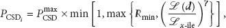
3.4. CSD Uplink Power Control

The considered uplink power control model is adopted from the LTE device uplink power control that can be formulated (in a linear scale) as follows with given parameters (listed in Table 1) [17]:

$$\begin{array}{cc}& P_{\text{CS}{\text{D}}_i}=P_{\text{CSD}}^{\max }\times \min \left[\mathrm{1},\max \left\{R_{\min },{\left(\frac{ℒ\left(d\right)}{{ℒ}_{x\text{-ile}}}\right)}^{\gamma }\right\}\right],\end{array}$$

(9)

where $R_{\min }=P_{\text{CSD}}^{\min }/P_{\text{CSD}}^{\max }$ and this is equivalent to $R_{\min }=P_{\text{CSD}}^{\min }-P_{\text{CSD}}^{\max }$ in a dB scale which means the minimum power reduction ratio to prevent CSDs with good channels to transmit at very low power level and ${ℒ}_{x\text{-ile}}$ stands for the x-percentile path-loss (plus shadowing) value and this is set to 98.6525 dB.

Table 1

Parameter settings.

Parameters	Settings
AL
(i) Transmit antenna gain, $G_{\mathrm{AL},\text{TX}}^{\mathrm{0}}$ (unit: dBi)	$\mathrm{12}$
(ii) Receive antenna gain, $G_{\mathrm{AL},\text{RX}}^{\mathrm{0}}$ (unit: dBi)	$\mathrm{12}$
(iii) Transmit power, $P_{\mathrm{AL}}$ (unit: dBm)	$\mathrm{12}$
(iv) Half-power beamwidth, ${\mathrm{\theta }}_{\mathrm{3}}^{\mathrm{AL}}$ (unit: °)	$\mathrm{60}$
Camera-sensing device (CSD)
(i) Transmit antenna gain, $G_{\text{CSD},\text{TX}}^{\mathrm{0}}$ (unit: dBi)	$\mathrm{6}$
(ii) Max. transmit power, $P_{\text{CSD}}^{\max }$ (unit: dBm)	$\mathrm{6}$
(iii) Min. transmit power, $P_{\text{CSD}}^{\min }$ (unit: dBm)	$-\mathrm{40}$
(iv) Half-power beamwidth, ${\mathrm{\theta }}_{\mathrm{3}}^{\text{CSD}}$ (unit: °)	$\mathrm{60}$
Carrier frequency, $f_c$ (unit: GHz)	$\mathrm{60}$
Bandwidth, B (unit: gigabit/s (Gbps))	$\mathrm{2.16}$
Reference distance, $d_{\mathrm{0}}$ (unit: m)	$\mathrm{1}$
The number of clusters	$\mathrm{19}$
The number of CSDs in a cluster	$\mathrm{5}$
Cluster radius (unit: m)	$\mathrm{50}$

4. Capacity Simulation Results

4.1. Analysis of Channel Capacity Simulation

For our simulation study, the corresponding parameter setting is as shown in Table 1. The nineteen CHs are deployed in the target network field in the feature of hexagonal cells. In each cell, five CSDs are uniformly deployed. The position of AL TX is near the hexagonal cells and the position of AL RX is 1000 meters far from the AL TX.

The simulation is performed while the position of AL TX varies from origin until 300 meters from the origin. The position of the origin is illustrated in Figure 6. According to the fact that the positions of CSDs are random within the associated cells, the corresponding directions of antenna radiation pattern are also not deterministic. Therefore, Monte Carlo simulation is performed and the number of Monte Carlo iterations is 50.

Figure 6

A reference simulation topology.

If the computed capacity based on Monte Carlo simulations with (4) is near 1.5 Gbps, uncompressed 1080p @ 30 Hz high-definition wireless video streaming is available [8, 9]. For an enhanced mode, we have to transmit 60 frames in a second; that is, 3 Gbps is required for uncompressed 1080p @ 60 Hz high-definition wireless video streaming.

The first simulation is performed with various numbers of CSDs in a cell as plotted in Figure 7(a). As can be seen in Figure 7(a), if 4 CSDs are deployed in each cell and if the AL TX is around 50 m (or more) far from the origin position, uncompressed 1080p @ 30 Hz high-definition video transmission is available. In addition, if 7 CSDs are deployed in each cell and if the AL TX is around 170 m (or more) far from the original position, uncompressed 1080p @ 30 Hz high-definition streaming is available. Last, the position of AL TX is approximately 280 m (or more) far from the original position and uncompressed 1080p @ 30 Hz high-definition streaming is possible when there are 10 CSDs in each cell. If more CSDs are located in a cell, they generate more interference to the AL TX, that is, to the AL wireless link. Thus, the smaller number of CSDs is beneficial in terms of the quality of video streaming in the AL wireless link. Moreover, if the position of AL TX is far from the set of CHs, the capacity of the AL wireless link is monotonously increasing because the interferences are attenuated due to the path-loss models.

Figure 7

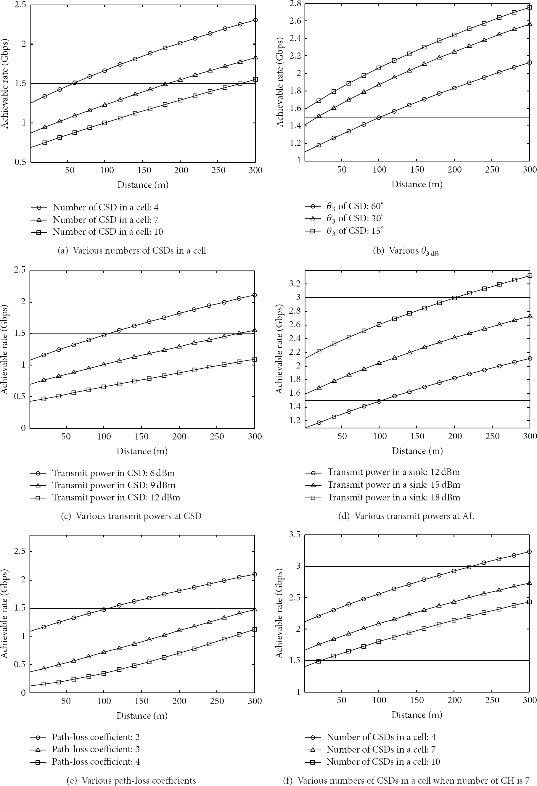
Simulation results.

The next simulation is performed with various ${\theta }_{\mathrm{3}\hspace{0.17em}\text{dB}}$ , that is, $\mathrm{1}{\mathrm{5}}^{\circ }$ , $\mathrm{3}{\mathrm{0}}^{\circ }$ , or $\mathrm{6}{\mathrm{0}}^{\circ }$ , as plotted in Figure 7(b). As can be seen in Figure 3, if ${\theta }_{\mathrm{3}\hspace{0.17em}\text{dB}}$ is narrow, the interference impacts should be limited. Therefore, the impacts on the AL wireless link is also limited if the ${\theta }_{\mathrm{3}\hspace{0.17em}\text{dB}}$ is narrow as shown in Figure 7(b). If the ${\theta }_{\mathrm{3}\hspace{0.17em}\text{dB}}$ of the AL wireless link is $\mathrm{1}{\mathrm{5}}^{\circ }$ , then the interference impacts are much less than the others; that is, the AL wireless link can always achieve more than 1.5 Gbps. Thus, it can always be available for 1080p @ 30 Hz uncompressed high-definition wireless video streaming. If ${\theta }_{\mathrm{3}\hspace{0.17em}\text{dB}}=\mathrm{3}{\mathrm{0}}^{\circ }$ or $\mathrm{6}{\mathrm{0}}^{\circ }$ , when the AL TX is around 20 m (or more) or 100 m (or more) far from the origin position, uncompressed 1080p @ 30 Hz wireless high-definition video transmission is available, respectively.

The simulation results with various transmit powers at CSD are plotted in Figure 7(c). As can be seen in Figure 7(c), if the transmit power at CSD is high, it generates higher interferences on the AL wireless link; that is, it highly interferes the AL wireless link. Thus, if the transmit power at CSD is 12 dBm, there is no chance to do uncompressed 1080p @ 30 Hz wireless video streaming. If the transmit power at CSD is 9 dBm, uncompressed 1080p @ 30 Hz video streaming is available when the AL TX is located at 300 m (or more) far from the original position. Last, uncompressed 1080p @ 30 Hz video streaming is realized if the AL TX is located at 110 m (or more) far from the original position when the transmit power of CSD is 6 dBm.

The other simulation is performed with various transmit powers at AL TX. If the power is high, it increases the signal strength, in turn; it also increases the capacity of the AL wireless link. As can be observed in Figure 7(d), if the transmit power of AL TX is 18 dBm, 1080p @ 60 Hz high-definition video streaming is available when the position of AL TX is 200 m (or more) far from the origin. When the transmit power is 15 dBm or 18 dBm, the AL wireless link can achieve 1080p @ 30 Hz high-definition wireless video transmission. If the transmit power of AL TX is 12 dBm, 1080p @ 30 Hz high-definition wireless video transmission is available when the AL TX is located in 100 m (or more) far from the origin position.

The next simulation is performed with various path-loss coefficients as can be seen in Figure 7(e). If the path-loss coefficient is high (i.e., 4), the achievable rate is low. If the path-loss coefficient is 2, 1080p @ 30 Hz high-definition video streaming is available when the position of AL TX is 100 m (or more) far from the origin. If the path-loss coefficient is 3, 1080p @ 30 Hz high-definition video streaming is available when the position of AL TX is 300 m (or more) far from the origin.

The last simulation is performed with various numbers of CSDs in a cell when the number of CHs is 7 (i.e., only white 7 cells exist in Figure 6) as plotted in Figure 7(f). All parameter settings are equivalent to the simulation results in Figure 7(a); however the number of CHs are different. As can be seen in Figure 7(f), if there is small number of CHs, the number of associated CSDs is decreased as well. Thus, the interference impacts are reduced; therefore, the overall capacity at the AL link increases. If the numbers of CSDs in a cell are 4 or 7, 1080p @ 30 Hz uncompressed video streaming is available. If the distance between AL TX and the origin is more than 230 meters, then 1080p @ 60 Hz uncompressed video streaming is also available. When the number of CSDs in a cell is 10, 1080p @ 30 Hz uncompressed video streaming is available if the distance between AL TX and the origin is more than 30 meters.

4.2. Quality Analysis of Massive Video Streaming

This section presents analysis results of video quality in two-tiered embedded camera-sensing systems using channel capacity simulation as performed in Section 4.1. The video quality analysis can be used for cell planning with appropriate admission control mechanisms to guarantee the certain level of video quality.

As shown in the channel capacity simulation in Section 4.1, video streaming at the AL wireless link is able to exploit full high-definition video streaming when the achievable rate is higher than 1.5 Gbps. However, if the distance between cells and a AL TX is near, the achievable rate is lower than the 1.5 Gbps due to the interference impacts that are simulated in Figure 7. To deal with the issue, light-weight sampling and coding methods are required. It is obvious that introducing entropy coding achieves 50% lossless compression [18]; that is, 750 Mbps is required for the full high-definition video streaming with the entropy coding. The computational complexity of the entropy coding is about 2% of overall video encoding [19] in the most recent video standard, high efficiency video coding (HEVC) [20]. Moreover, introducing 4 : 2 : 0 YUV chroma subsampling allows additional 50% bit rate reduction without noticeable impacts on human visual perception. Therefore, the rate of 375 Mbps can guarantee the full high-definition video streaming without noticeable quality degradation.

As can be observed in Figure 7, most of the achievable rates are more than 375 Mbps. However, if the number of CSDs in a cell is more than 10, the rate can be lower than 375 Mbps. Thus, additional light-weight lossy coding methods are required for the video streaming under the rate of 375 Mbps. It is also known that the spatial downsampling maintains good quality of experience (QoE) until the downsampling ratio is less than 50% while the temporal downsampling provides lower QoE. To quantify the effect of video quality degradation, five 1080p sequences (ParkScene, Kimono, Cactus, BasketballDrive, and BQTerrace) of the common test condition [21] defined in the HEVC video standard are used with 14 points of downsampling ratios between 100% and 0%.

Table 2 and Figure 8 show the video quality degradation according to the spatial downsampling. In Table 2 and Figure 8, the ratio 100% represents the original resolution video that is not spatially downsampled. The spatial downsampling degrades video qualities linearly, and the PSNR difference is lesser than 6 dB until the downsampling ratio is more than around 60%. The quality degradation is highly depend on the original video quality and can be estimated by the following linear regression analysis. By calculating the linear regression analysis with Table 2, the video quality degradation (VQD; difference between original quality and downsampled quality) in PSNR can be represented as following equation:

$$\begin{array}{cc}& \text{VQD}=-\mathrm{0.08}\times R_{\text{ds}}^{\mathrm{3}}+\mathrm{0.21}\times R_{\text{ds}}^{\mathrm{2}}-\mathrm{2.79}\times R_{\text{ds}},\end{array}$$

(10)

where $R_{\text{ds}}$ stands for the spatial downsampling ratio.

Table 2

Y-PSNR values according to the ratio of spatial downsampling.

Downsampling ratio	Resolution	Sequence name					Average
		ParkScene	Kimono	Cactus	BasketballDrive	BQTerrace
100%	$\mathrm{1920}\times \mathrm{1080}$
93%	$\mathrm{1792}\times \mathrm{1008}$	41.36	45.71	39.79	38.94	36.09	40.38
87%	$\mathrm{1664}\times \mathrm{936}$	41.16	45.61	39.58	38.74	35.90	40.20
80%	$\mathrm{1536}\times \mathrm{864}$	40.61	45.15	39.07	38.32	35.44	39.72
73%	$\mathrm{1408}\times \mathrm{792}$	37.55	43.29	36.11	35.64	32.57	37.03
67%	$\mathrm{1280}\times \mathrm{720}$	37.36	43.19	35.91	35.46	32.37	36.86
60%	$\mathrm{1152}\times \mathrm{648}$	35.82	42.13	34.82	34.17	31.01	35.59
53%	$\mathrm{1024}\times \mathrm{576}$	34.95	41.40	33.52	33.39	30.05	34.66
47%	$\mathrm{896}\times \mathrm{504}$	33.45	40.37	32.04	32.06	28.55	33.29
40%	$\mathrm{768}\times \mathrm{432}$	33.05	39.96	31.68	31.74	28.18	32.92
33%	$\mathrm{640}\times \mathrm{360}$	31.29	38.45	30.03	30.27	26.51	31.31
27%	$\mathrm{512}\times \mathrm{288}$	30.69	37.63	29.50	29.80	25.99	30.72
20%	$\mathrm{384}\times \mathrm{216}$	29.13	35.37	28.10	28.53	24.69	29.16
13%	$\mathrm{256}\times \mathrm{144}$	27.36	32.26	26.40	26.95	23.24	27.24
7%	$\mathrm{128}\times \mathrm{72}$	24.35	27.12	23.29	23.97	20.81	23.91

Figure 8

The effect of video quality according to spatial downsampling.

Figure 9 shows the visual video quality comparison according to the spatial downsampling, and 67% of downsampling shows better quality of images compared to 33% of downsampling. Thus, in the cell planning, the number of acceptable CSD in a cell can be calculated by (10) with a predefined minimum video quality threshold (e.g., 35 dB in PSNR) for admission control and rate adaptation [22].

Figure 9

Video quality comparison according to the ratio of spatial downsampling; (a)–(c) BQTerrace, (d)–(f) Cactus, and (g)–(i) ParkScene.

5. Conclusions

This paper performs the quality analysis of high-definition video streaming in two-tiered embedded camera-sensing systems where the cameras are recording visual scenes in the network target fields and transmitting the video streams via IEEE 802.15.3c multigigabit wireless channels. In this scenario, the 60 GHz multigigabit wireless transmission introduces interference to the AL wireless link. This paper analyzes the capacity degradation on the main AL wireless link due to the interference by the wireless transmission from camera-sensing nodes. For more realistic performance evaluation in terms of channel capacity of the AL wireless link, IEEE 802.15.3c path-loss and azimuthal antenna radiation models are used. In addition, performance evaluation with actual video streams is also performed, presented, and analyzed to show real-world impacts in terms of video quality.

According to the simulation results of the estimated capacity and interference, we can provide the guideline for how much interference should be suppressed or mitigated with interference mitigation techniques. It means if one technique is able to suppress more interference than the quantitative value, the proposed technique is meaningful. Therefore, the simulation results in this paper provide quantitative guidelines for possible interference mitigation techniques.