
Abstract
We investigate three aspects of dynamicity in ad hoc and wireless sensor networks and their impact on the efficiency of intrusion detection systems (IDSs). The first aspect is magnitude dynamicity, in which the IDS has to efficiently determine whether the changes occurring in the network are due to malicious behaviors or or due to normal changing of user requirements. The second aspect is nature dynamicity that occurs when a malicious node is continuously switching its behavior between normal and anomalous to cause maximum network disruption without being detected by the IDS. The third aspect, named spatiotemporal dynamicity, happens when a malicious node moves out of the IDS range before the latter can make an observation about its behavior. The first aspect is solved by defining a normal profile based on the invariants derived from the normal node behavior. The second aspect is handled by proposing an adaptive reputation fading strategy that allows fast redemption and fast capture of malicious node. The third aspect is solved by estimating the link duration between two nodes in dynamic network topology, which allows choosing the appropriate monitoring period. We provide analytical studies and simulation experiments to demonstrate the efficiency of the proposed solutions.
1. Introduction
Multihop ad hoc wireless networks are a set of nodes equipped with wireless interfaces, and data are forwarded through multiple nodes to reach the intended destinations. They include many types of networks such as mobile ad hoc networks (MANETs) [1], wireless sensor networks (WSNs) [2], and vehicular ad hoc networks (VANETs) [3].
In the last decade, there has been a substantial research in the area of security in ad hoc and wireless sensor networks [4, 5]. The security solutions have been designed with the goal of protecting the networks against some attacks such as selective forwarding, black hole, wormhole, sinkhole, and energy exhausting attack. Prevention mechanisms like key management and authentication, which represent the first line of defense, are not sufficient to provide an efficient security solution. Therefore, there is a need to deploy a second line of defence named intrusion detection system (IDS).
In general, intrusion detection systems are divided into two major approaches: misuse detection and anomaly detection [6]. Misuse detection performs signature analysis by comparing on-going activities with patterns representing known attacks, and those matched are labeled as intrusive attacks. The misuse approach is showing its limits as it cannot detect new attacks. Anomaly detection, on the other hand, builds profile of normal behavior and attempts to identify the patterns or activities that deviate from the normal profile. The main advantage of anomaly detection is that it can detect unknown attacks.
The detection model that we consider in the ad hoc and wireless sensor network is as follows. The IDS is implemented in a distributed manner; each node can act as a monitoring node that observes the behavior of its neighbors. Each observation lasts for a monitoring time interval of duration Δ, called the monitoring period. The IDS can judge whether the monitored node is normal or anomalous after one or multiple consecutive observations.
Although intrusion detection systems have received considerable attention in ad hoc and wireless sensor networks [7, 8], to the best of our knowledge, there are no studies on the impact of network dynamicity on IDS efficiency and how the IDS can react or adapt to these changes.
In this paper, we investigate the following three aspects of behavioral dynamicity that occur in the network and can negatively affect the IDS performance and efficiency.
Magnitude Dynamicity. Due to change of user requirements, a node changes the rate at which it generates data. For instance, a legitimate user wants to change (i.e., increase/decrease) the data collection rate received at the sink node. The challenge facing the IDS here is to be efficient at detecting attacks and distinguishing between the changes due to normal behaviors and the changes due to malicious attacks.
Nature Dynamicity. In some detection models, a monitoring node has to observe the behavior of the monitored node during a set of consecutive monitoring periods before judging whether the monitored node is malicious or not. A monitored node might evade from IDS detection and confuses it by switching continuously its behavior between normal and anomalous. In this case, the malicious node strives to cause network disruption without being detected by the IDS.
Spatiotemporal Dynamicity. The IDS detection mechanism is based on collecting a set of consecutive observations about the monitored node. An IDS is able to observe the behavior of the monitored node if the latter stays within the monitoring node's transmission range for a duration exceeding Δ. By knowing this fact, a malicious node can evade IDS detection by moving around in the network at a speed, which prevents it from being within the monitoring node's transmission range for a duration higher than Δ.
In this paper, we propose a solution for each aspect of dynamicity mentioned above. The contributions of the paper are threefold. Firstly, the magnitude dynamicity aspect is solved by defining a normal profile based on the invariants derived from the normal node behavior. This is achieved by generating a dependency graph consisting of strongly correlated features and then derives the high-level features from the graph. The high-level features are obtained by applying the divide-and-conquer strategy on the maximal cliques algorithm and the maximum weighted spanning tree algorithm. Secondly, to handle nature dynamicity aspect, we adopt the carrot and stick strategy (i.e., reward generously and punish severely) to prevent a malicious node from evading the IDS. To do so, we propose an adaptive reputation fading strategy to allow fast redemption and fast capture of malicious node. Thirdly, we use statistical analysis to estimate the link duration between two nodes in dynamic network topology. Based on this estimation, the monitoring node chooses the appropriate monitoring period, which allows it to observe the monitored node's behavior.
The rest of the paper is organized as follows. In Section 2, we describe the normal profile construction and the feature selection method. Section 3 presents the adaptive reputation fading strategy. In Section 4, we analyze link-node duration in a mobile wireless network and explain how the monitoring time period is estimated. Finally, Section 5 concludes the paper.
2. Magnitude Dynamicity
2.1. Background
2.1.1. One-Feature Profile
In the one-feature profile, we use a single feature to describe and detect anomalous behavior. To detect the network malicious behavior, a node can measure the following features, as shown in Table 1 [9]. The disadvantage of this profile structure is that there is a need to assign one feature for each known attack. In this case, the IDS has to measure each feature and check whether it has anomalous value. When the number of attacks increases, the detection speed of the IDS becomes slow. It also becomes slower when the size of rule set increases.
Relation between attacks and features.

The one-feature profile might fail at distinguishing between normal and anomalous behaviors. Figure 1 shows that using some features individually to describe normal behavior is misleading and might make the detection system falsely accuse a legitimate node of being malicious. Figure 1(a) depicts a tree-based wireless network rooted at the sink B and it shows the normal traffic rates of the network. The value above each link indicates the flow rate traversing this link. Each node measures the flow rate coming from its upstream neighbors. Figure 1(b) (resp., Figure 1(c)) shows the state of the network when nodes D, H, and K become compromised and start behaving maliciously by dropping some packets (resp., generating more packets). As D, H, and K reduce (resp., increase) their sending rate, their respective downstream neighbors I and L have also to reduce (resp., increase) their sending rate accordingly. As a result, node B will falsely accuse nodes I and L of performing selective forwarding attack (resp., energy exhaustion attack), and hence a high false positive rate will be observed.

Impact of feature choice on false positive rate.
2.1.2. Multifeature Profile
In the multifeature profile, we describe the normal behavior by a d-feature vector and each element of the vector represents a feature. In this way, the IDS can determine whether some features together show an anomalous behavior. Experiments have shown that we can obtain better detection accuracy by combining related features rather than individually [10]. If node B in the example of Figure 1 considers two features: (a) the flow entering the monitored node and (b) the flow leaving the monitored node, it will conclude that nodes I and L are just forwarding what they received from their upstream neighbors, and hence they are not malicious.
Loo et al. [11] group the observed data into clusters and use a profile of 12 features to describe normal profile. To check whether a test instance belongs to a given cluster, they measure the Euclidian distance between the test point and the centroid of the cluster. If such a distance is higher than a threshold distance, the test point is considered anomalous. The following example shows that the Euclidian distance between two d-feature profiles reduces the detection accuracy. Let
In [9, 12], the normal profile of a monitored node i is defined by a q-feature vector
2.2. Profile Construction Based on Strongly Correlated Features
When it comes to comparing distances, we find that the Mahalanobis distance is a powerful technique as it takes the covariances into account, which leads to elliptic decision boundaries in the 2D space. While the Euclidean distance builds circular boundaries and considers equal variances of the features, it appears that the Mahalanobis distance is more appropriate for multivariate data.
In our paper, we take a novel approach to select relevant features and construct the normal profile vector. We do not assume multivariate normal distribution and we feed only strongly correlated features to the distance measure unlike the Mahalanobis distance, which considers correlation between all features.
In the training phase, we investigate the significant associations between features. We are interested in identifying the level of correlation between those features, called Pearson's correlation coefficient, which measures the strength of the linear association between features. Pearson's correlation coefficient between two feature vectors X and Y is defined by

where
The Pearson correlation indicates to what extent variables show a linear relationship (correlation) among them. The correlation takes its values in the range from −1 to +1. The extreme value +1 (resp., −1) informs about a perfect direct/increasing linear relationship (resp., inverse/decreasing). Indeed, strong relationship between variables is reflected by values close to the limits (
In our approach, we first use the training dataset F represented by
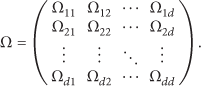
We consider the set of d feature vectors
A subgraph
The induced graph
We aim at finding the set of features that increase and decrease altogether in order to avoid the missed detection problem as in [11]. The best way to do so is to extract from G the set of cliques composed of strongly correlated features. One of the widely adopted solutions [15] to compute maximal cliques in an arbitrary graph of d vertices runs in time

By applying the same algorithm on each connected partition of
Let ϕ be the set of edges belonging to all cliques in
The high-level features belonging to the same clique
To illustrate further the above method, we consider an example of seven network features, namely,

According to the correlation matrix, we generate the graph
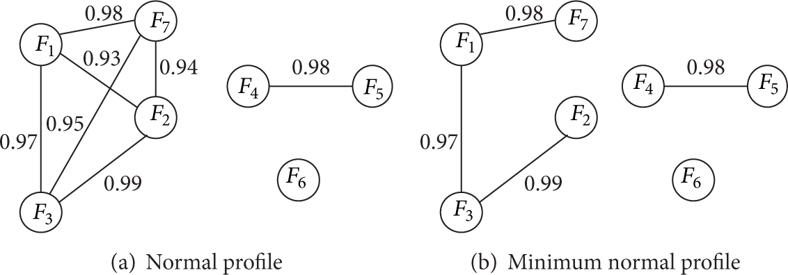
Graph-based normal behavioral model.
The network normal profile is defined as
Proposition 1.
For any data set of d low-level features, the number of high-level features induced by the graph-based generation method is upper-bounded by
Proof.
Consider
2.3. Detection Process
Each node constructs its local dataset represented by
To check whether a profile Z is normal or anomalous, we derive from Z its corresponding high-level profile
(1) Let Z be the high-level test profile composed of (2) (3) (4) return Z is anomalous (5) (6) (7) return Z is normal;
2.4. Simulation Results
We study the performance of the proposed IDS using GloMoSim simulator [17]. Each node sends one packet/sec toward the sink. A watchdog is implemented at each node and its role is to monitor the network activities of all the node's neighbors. At every 10 seconds (i.e., one time period), a monitoring node i measures the feature vector of its monitored node j. After a training phase of T time periods, testing phase lasts for 1800 seconds. The role of IDS, which is implemented at a node i, is not just to detect if i's neighbor (node j) is malicious or not but also to detect if node j is malicious during a given time period. We evaluate the performance of the IDS using two metrics: detection rate and false positive rate. We select the following five quantitative features:
number of generated packets (GEN),
number of received packets (RCV),
number of forwarded packets (FWD),
number of sent packets (SENT),
number of lost packets (LOSS).
We generate then the correlation matrix Ω as well as the minimum normal profile after performing the maximal cliques algorithm and the maximum weighted spanning tree algorithm as shown in Figure 3:
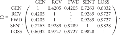

Normal profile and minimum normal profile.
Figure 4 shows the detection rate of the proposed IDS as a function of dropping probability. The first observation that we can draw from the figure is that the detection rate is 100% when the dropping probability is higher than 0.05, and it is under 100% when the dropping probability is

Detection rate versus dropping probability.

Detection rate versus training time.
Figure 6 shows the false positive rate of IDS as a function of training period under the following levels of dropping probability
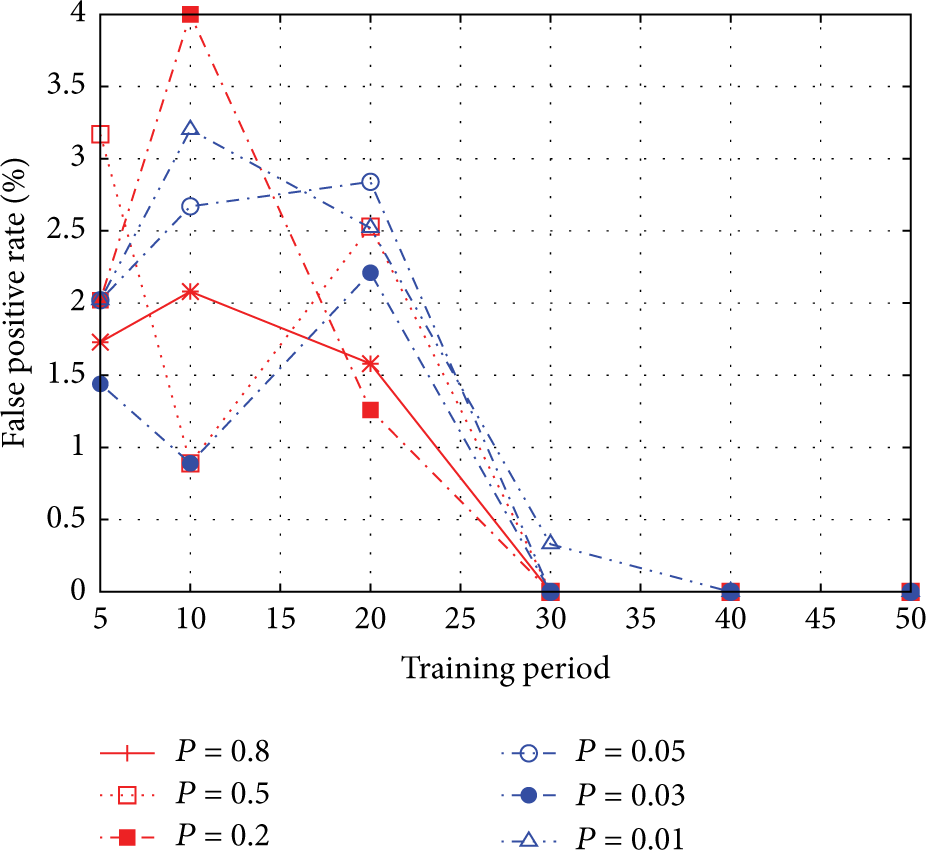
False positive rate.
3. Nature Dynamicity
3.1. Background: Constant Fading Reputation Strategy
Reputation is defined as the general opinion of a society of nodes towards a certain node in a specific domain of interest, and it is the global perception on the future behavior of this node. In the IDS based on multiple observations, the IDS collects a series of consecutive observations, each of which occurs during a separate monitoring period.
Since reputation aggregates past experiences and dynamically evolves, it is similar to Bayesian analysis, which is a statistical procedure that estimates parameters of an underlying distribution based on observations. Starting with prior distribution, which is the initial state before any observation is made, Bayesian analysis continuously takes into account new experiences and derives posterior probability [18]. One of the used distributions in Bayesian analysis is Beta distribution.
Beta distribution has been recognized as a useful formal tool to model reputation [18–20]. A reputation value assumes a tuple of
The Beta distribution and its probability density function (PDF) are defined as follows:
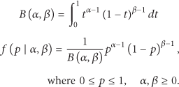
The reputation, denoted by R, is defined as the expectation (denoted by

We model the reputation of a node with a Beta distribution (
The standard Bayesian procedure is as follows. Initially, the prior is
If the observation is qualified as misbehavior, β is set to
If the observation is qualified as correct behavior, α is set to
The standard Bayesian method is modified in [19] to give less weight to the observations received in the past so as to allow reputation fading and prevent any node from capitalizing on its previous good behavior forever. To achieve this aim, a discount factor for past observations is used. When a new observation
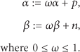
The weight ω is a constant discount factor for past observations, which serves as the fading mechanism. We refer hereafter to the reputation system described above as the constant fading reputation strategy.
3.2. Adaptive Fading Reputation Strategy
The constant fading reputation mechanism uses the same discount factor for all types of observations and during all the time. The higher (resp., lower) the value of ω is, the slower (resp., quicker) the histories are forgotten. By knowing the value of ω, a malicious node can evade from IDS detection by misbehaving for a given time and goes back to normal behavior. Under high discount factor, the change of node behavior (from well-behaved to misbehaved and vice versa) will be detected after a long time. During this time, well-behaved nodes can count on their good histories and act maliciously. In addition, misbehaved nodes will have to wait a longer time to redeem themselves. On the other hand, a low discount factor permits a quicker detection redemption of nodes. However, it might raise false alarms especially when network faults and attacks both share the same failure symptoms. For instance, a misbehavior is detected if the observed node is not forwarding a packet. This rule is set to detect black hole and selective forwarding attacks. In addition, this rule is applied when packets are not forwarded due to collisions, which means that a well-behaved observed node might be falsely considered malicious.
To deal with this issue, we propose an adaptive fading reputation mechanism. This mechanism uses the carrot and stick strategy; that is, reward the well-behaved node and punish the misbehaved node. The adaptive mechanism uses two types of discount factors: one for past positive observations and the second one for past negative observations. The value of the discount factors is adjusted as function of reputation R as shown in Figure 7.
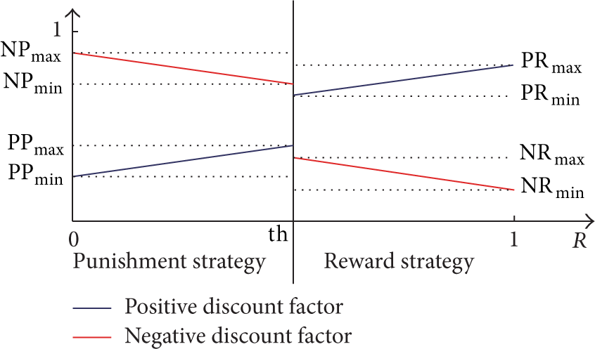
Positive and negative discount factors.
In the adaptive fading reputation mechanism, when a new observation

Reward Strategy. It is applied when the reputation
Punishment Strategy. It is applied when the reputation
Formally,
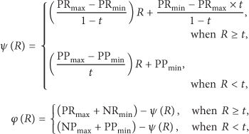
where
For new nodes, positive and negative histories are kept with a discount factor equal to 1 when the number of observations is less than a given value named experience threshold.
From the above upper and lower bounds, we define the following two distance metrics.
Punish-to-Reward (PTR) Distance. It is defined by
Reward-to-Punish (RTP) Distance. It is defined by
3.3. Performance of Adaptive Discount Factor Strategy
We evaluate the performance of the constant and adaptive discount factor strategies in terms of detection time. To do so, we implement three behavioral models.
Deterministic redemption model: in this model, a node with reputation
Deterministic evasion model: in this model, a node with reputation
Probabilistic evasion model: the node's behavior is modeled with a two-state Markov chain as depicted in Figure 8. In state N, the node is well-behaved, and, in state M, the node is misbehaved. Initially, the node's reputation

Probabilistic evasion model.
The parameters for the experiment are shown in Table 2. We define three settings for the adaptive fading reputation.
Setting 1:
Setting 2:
Setting 3:
Experiment parameters.

As for constant fading reputation, we define three levels of discount factor
We study the evolution of reputation over time when applying constant and adaptive discount factor. In Figure 9(a), the convergence time increases as ω increases. This is because higher (resp., lower) values of ω mean that the negative histories are forgotten at slower (resp., faster) rate, which leads to longer (resp., shorter) time to converge to

Deterministic redemption model.
In Figure 10, we also notice that the malicious node that follows the deterministic evasion is detected more quickly when the adaptive discount factor strategy is applied. The time to converge to

Deterministic evasion model.
By knowing the required number of observations to detect a malicious node, the latter can adopt the probabilistic evasion model, which do discontinuous harm to the network to confuse the IDS and hence evade detection. Figures 11, 12, and 13 show that the adaptive discount factor strategy can quickly detect this type of behavior. In the figures, we consider that a node is malicious when

Probabilistic evasion model (

Probabilistic evasion model (

Probabilistic evasion model (
4. Spatiotemporal Dynamicity
A monitoring node i can make at least one observation about a monitored node j if the wireless link lasts for a duration higher than the monitoring period Δ. The malicious node j, which knows this fact, can move around in the network to create links with its neighbors of duration less than Δ.
As shown in Figure 14, the nodes start operating at time

Link-node lifetime.
In this section, we statistically analyze the link-node distribution. Based on this analysis, we choose appropriate values for the monitoring period so that the mobile monitored node cannot evade IDS detection. We use the random waypoint mobility model, in which each mobile node randomly selects a location, within an area of 100 m × 100 m, with a random speed uniformly distributed between 0 and a certain maximum speed
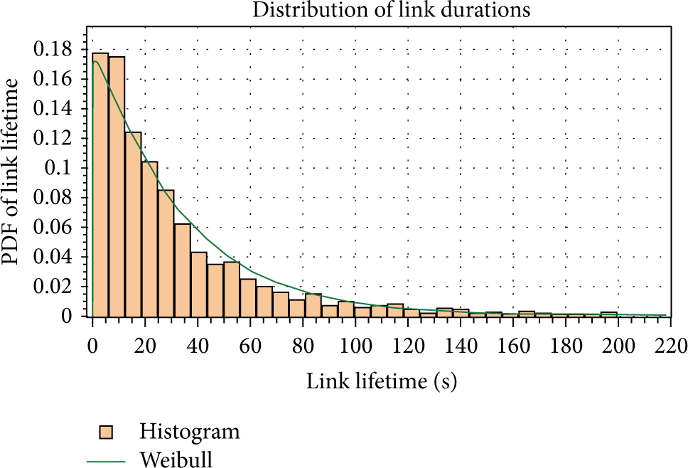
4.1. Link Lifetime Distribution
We obtain from our simulation the frequency of link durations and plot them into a histogram, as shown in Figures 15 and 16. The EasyFit software [21, 22] is used to measure the compatibility of a random sample with the theoretical probability distribution functions. As shown in the figures, the software approximates the simulation data to a Weibull distribution [23] with two parameters


Link lifetime distribution under
Link lifetime distribution under
Based on the properties of the Weibull distribution, the mean (expected value) is

On the other hand, Samar and Wicker [24, 25] have described the expected link lifetime as a function of node velocity, say

where R is the radius of the circle centered at the node.
Since (12) and (13) are both describing the expected value of the link lifetime, we can write

We derive then β as a function of velocity

Simulations have been conducted to compare between the theoretical β obtained from (15) and the Weibull approximative one obtained from simulations, as shown in Table 3. The results show that the Weibull distribution fits well simulation data.
Comparison between theoretical and approximative β.

4.2. Residual Node Lifetime Distribution
We assume that the node lifetime follows an exponential distribution with a parameter λ. This distribution is similar to the one used to model “time to failure” in reliability engineering. We consider that λ is the rate at which node's battery is discharged. The probability density function is then

The probability density function of the residual node lifetime for a node of age a is given by the following equation [26]:
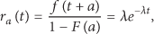
where F is the cumulative density function (CDF) of the exponential distribution. Thus, the residual node lifetime also follows an exponential distribution. The expected value for the random variable X following an exponential distribution is

4.3. Link-Node Lifetime Distribution
Consider a random variable Z, where

Therefore,

Consequently, the cumulative distribution function (CDF) of Z is

Thus,

The approximated density function for the combined variables X and Y is a Phased Bi-Weibull distribution [27], which has a PDF as shown in

EasyFit software [22] approximates the simulation data to the Phased Bi-Weibull distribution, as shown in Figure 17 (resp., Figure 18), with parameters

Link-node lifetime distribution under

Link-node lifetime distribution under
Remark 2 (see [28]).
For real values
The result of this remark is extended to random variables by the following theorem.
Theorem 3 (see [28]).
Given two real-valued continuous random variables X, Y
Lemma 4 (see [28]).
Given two real-valued continuous random variables X, Y
Based on Theorem 3 and Lemma 4, the expected link-node lifetime is given by

where

Expected link-node lifetime.
4.4. Monitoring Period Estimation
Based on the above statistical analysis, we propose a method to choose the appropriate value for the monitoring period. This method is low-cost and more appropriate for resource-constrained networks like sensor networks. We also propose another method that requires some communication cost and can be implemented on nodes with higher capabilities such as mobile sinks or mobile ad hoc networks and vehicular ad hoc networks.
4.4.1. Low-Cost Method
We assume that the monitoring node has no information about the monitored node's velocity, position, or residual battery, and it wants to ensure that
4.4.2. High-Cost Method
We assume that each node i can estimate its remaining battery power
Each node i periodically broadcasts a beacon message containing its residual node lifetime

After that, each node j estimates the residual link-node lifetime given by

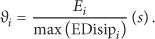
Therefore, the monitoring period required to observe the monitored node i must be less than
5. Conclusion
In this paper, we have proposed IDS solutions for three aspects of dynamicity in ad hoc and wireless sensor networks. The magnitude dynamicity aspect is solved by defining a normal profile based on the invariants derived from the normal node behavior. We have generated a dependency graph consisting of strongly correlated features, and we have derived the high-level features from the graph. The high-level features are obtained by applying the divide-and-conquer strategy on the maximal cliques algorithm and the maximum weighted spanning tree algorithm. Simulation results show that the IDS can achieve a detection rate of 100% when the malicious behavior is not similar to the normal one. In addition, it can also achieve a false positive rate of 0% when the duration of the training time exceeds a given value. To handle nature dynamicity aspect, we have adopted the carrot and stick strategy to prevent a malicious node from evading the IDS. To do so, we have proposed an adaptive reputation fading strategy to allow fast redemption and fast capture of malicious node. We have analytically studied link-node lifetime distribution and have shown that it can be approximated to the Phased Bi-Weibull distribution. Based on this analysis, we have proposed a low-cost method to estimate the minimum monitoring period required to observe the monitored node's behavior. In addition, based on some topology information, we have proposed a high-cost method designed for network having nodes less constrained with resource limitations.
Footnotes
Conflict of Interests
The authors declare that there is no conflict of interests regarding the publication of this paper.
Acknowledgment
The authors would like to extend their sincere appreciation to the Deanship of Scientific Research at King Saud University for funding this research through Research Group Project (RG no. 1435-051).