A Graph Embedding Method Based on Sparse Representation for Wireless Sensor Network Localization

Abstract

In accordance with the problem that the traditional trilateral or multilateral estimation localization method is highly dependent on the proportion of beacon nodes and the measurement accuracy, an algorithm based on kernel sparse preserve projection (KSPP) is proposed in this dissertation. The Gaussian kernel function is used to evaluate the similarity between nodes, and the location of the unknown nodes will be commonly decided by all the nodes within communication radius through selection of sparse preserve projection self-adaptation and maintaining of the topological structure between adjacent nodes. Therefore, the algorithm can effectively solve the nonlinear problem while ranging, and it becomes less affected by the measuring error and beacon nodes quantity.

1. Introduction

For most wireless sensor network (WSN) applications, it is essential to know the location of sensor nodes. Related researches show that, in the information related to the context of monitoring deployment area provided to the users, more than 80% is related to the information of location [1].

The self-localization algorithm of nodes can be divided into the two major categories: range-based and range-free [2, 3]. Range-based approaches have a relatively higher accuracy, but this final location estimation accuracy depends on the measuring accuracy. The most common measuring technologies include Radio Signal Strength (RSSI) [4], Time of Arrival (ToA) [5], Time Difference of Arrival (TDoA) [6], and Angle of Arrival (AoA) [7]. The measurement data of RSSI can be achieved during each data communication between nodes, and it does not occupy additional bandwidth and energy, so the hardware expense is relatively simple and cheap. These turn it into a hotspot research direction to use the RSSI measurement data to conduct localization. However, in a complicated monitoring environment, the measurement of RSSI signal is also affected by multiple factors; for example [8–10], the communication between nodes generally uses free common channel, which is inevitably interfered by other devices in the monitoring area; RSSI signal itself has multipath feature; the hardware of sensor node is relatively cheap, simple, and with poor operational capability, and in addition, the unstable production technique has also caused unstable quality of certain node products, blockage by static or moving obstacles in the monitoring area, and so forth. All these will provoke a large amount of uncertain factors in the collected signals and make the signal present nonlinearity.

Figure 1 shows the cause of nonlinearity in a complex environment. When the part between node A and node C is interfered by other devices of the same frequency band, or if it is blocked by a static or moving object, the measured value is generally bigger than the actual value. If only linear method is used without considering the actual environment, and if the empirical model is directly used to obtain the measuring distance, the measuring precision is generally very low, which obviously cannot satisfy the actual application. Therefore, there are multiple difficulties to face in order to obtain accurate localization, which requires exploring new technologies and methods or combining other solutions to handle it.

Figure 1

Distance measurement in complex environment.

The rest of the paper is structured as follows. In Section 2, we address the related work in the area of range-based localization schemes. In Section 3, we give a brief review of related concepts. And Section 4 presents our localization method. Section 5 shows simulated results, and Section 6 gives the conclusions.

2. Related Work

Related literature [11] generally divides the localization algorithm based on signal strength ranging into two types: one type uses empirical formula transformation to obtain the distance after obtaining the signal strength between nodes and then uses the trilateration method or multilateral method to obtain the location of unknown node; another type directly uses the signal strength information between nodes to obtain the similarity between nodes through the machine learning method, and then, the relation between nodes is mined in accordance with the similarity and the location of beacon node. The former depends on the empirical model, and classic methods include the RADAR system [12] and SpotON system [13]. They only can be applied to some scenarios with relatively unchanging environment, and in order to obtain the localization result with high accuracy, training calibration should be conducted to different environments, which might cost a large amount of manpower and material resources. If the fitting model is not accurate or the deployment scenario is modified, then the original model cannot reflect the relation between the Euclidean distances and RSSI values, the distance measurement accuracy is low, and it will result in undesirable localization effects. The latter regards the nodes in network as independently distributed devices, uses the RSSI measurement values between adjacent nodes, refers to the machine learning algorithm, trains and learns a prediction model in the deployment area, and further estimates the location information of unknown nodes in the area, such as the LANDMARC localization system based on k nearest neighboring (k-nn) [14], kernel principal component analysis (KPCA) localization algorithm [15], kernel canonical correlation analysis (KCCA) location estimation method [16, 17], and localization algorithm based on kernel locality preserving projection (KLPP) [18]. The range-based localization technology based on machine learning method is not sensitive to RSSI measurement error and it has the characteristics of low requirement for measurement technology and high self-adoption degree; therefore, it has attracted considerable attention.

The k-nn method [18] relies on the “nearest adjacent distance criteria” weighted idea to obtain the information of unknown nodes, its algorithm is a kind of linear algorithm, the k value is generally artificially set, and it has high randomness. In addition, when the nodes are assigned to a complicated environment, the RSSI measured values have a high nonlinearity, which would lead to poor localization result. For nonlinear data, the researchers find that it is a practical and effective solution to use the kernel method to build the mapping model. The kernel method [19, 20] maps the original data into an appropriate high-dimensional feature space through a certain suitable kernel function, which transfers the nonlinear problem difficult to solve in the original space into a linear problem in the feature space. By referring to the characteristics of the kernel method, this paper uses it to solve the nonlinear problem in the RSSI measured data.

A large number of related researches show that after kernel function and training set are given, the kernel matrix (or Gram matrix) can be built, and the real internal structure of data can be disclosed in accordance with the similarity provided by the kernel matrix. The KPCA and KCCA localization algorithms taking into account this theory have been proposed successively.

KPCA is an extension of principal component analysis (PCA) [21] using techniques of the kernel method. Using kernel method, the nonlinear data is mapped into a high-dimensional feature space and then PCA is employed in feature space. The linear PCA in the high-dimensional feature space can best represent the projection of original data in order to realize dimensionality reduction and denoising of data. KCCA is also a kind of dimensionality reduction method similar to KPCA, and different from KPCA; by building the mapping of signal space and physical space in the feature space, the localization method based on KCCA makes it possible for the nodes to use RSSI values to deduce back the relative topological structure of their physical space and then calculate the location of these nodes. However, both of the KPCA and KCCA computations have adopted a global nonlinear mapping algorithm, which is simple and highly efficient, and although it can obtain good results under some situations, it has ignored the data distribution and failed to consider that the data have the local distribution feature. In addition, the KCCA algorithm is only applicable to fingerprint-based database for indoor localization, and it requires artificially collecting the training datum and building the distribution diagram of the relation between RSSI and Euclidean distances beforehand. During localization, in accordance with the distribution diagram obtained during previous training, k nearest access points (APs) will be found, and their center of mass will be used as the estimated location, and if the APs density is not high enough, it requires further iterative operation. Therefore, the KCCA estimation algorithm does not apply to the random deployment environment or any scenarios that cannot be reached by human.

Based on that, Wang et al. [18] used the KLPP algorithm and proposed the KLPP-based localization algorithm. The KLPP localization method uses the kernel function to measure the similarity between nodes, and after the RSSI values are mapped into the feature space, it uses the LPP algorithm [22] to construct the adjacency graph between nodes, which formulates the localization problem as a graph embedding problem and allows us to consider the topological structure of the networks. The KLPP-based localization method uses the kernel method to solve the nonlinear problem of RSSI values; by using the adjacency graph, the location of unknown nodes is commonly decided by their adjacent nodes, so the measurement error caused by remote beacons during the process of traditional multilateral or trilateral method is avoided, and the impact by the number of beacon nodes is small.

However, the KLPP algorithm is overly dependent on the adjacency graph, while the construction of the adjacency graph mainly use k-nn and  ε-ball approaches [23]. The k-nn and  ε-ball methods are the two most popular ones for graph construction in the literature. The k-nn graph method chooses k nearest adjacent samples, while the ε-ball method chooses the samples which falling into its ε-ball neighborhoods are linked to it. In addition, the weight of side in the graph is generally obtained through methods like binary, Gaussian kernel, or ${\mathcal{l}}_{\mathrm{2}}$ -reconstruction [24–26]. All of them determine the neighboring data based on the pairwise Euclidean distance, which is, however, very sensitive to data noises, especially in high-dimensional spaces; that is, the graph structure may dramatically change the presence of noise. The construction of the adjacency graph and the choice and setting of weight all restrict the final localization result of KLPP-based algorithm. For the localization algorithm, once the adjacency graph between nodes is given, in the subsequent operation, the adjacency graph parameters might have no change at all. However, for the WSN, its deployment area is generally affected by various actual factors such as hardware error, network attacks, and lack of energy and severe weather, which causes that the network topology can change at any time. Therefore, it is difficult for the KLPP-based localization method with preset parameters to adapt to a complicated environment, and as showed in Figure 1, when it is affected by the interference source, the structure in the figure will be affected in a certain degree. How to self-adaptively determine the relation between nodes is the foundation to obtain satisfying location estimation result. Researchers [27] found that sparse representation (SP) has natural discrimination ability, and through construction of ${\mathcal{l}}_{\mathrm{1}}$ -graph, each sample can automatically choose the adjacent samples through SP method and automatically make each sample be represented by the combination of surrounding training samples. In addition, ${\mathcal{l}}_{\mathrm{1}}$ -graph is robust owing to the overall contextual ${\mathcal{l}}_{\mathrm{1}}$ -norm formulation and the explicit consideration of data noises. Qiao et al. [28] smartly applied SP to the structure of the adjacency graph and proposed the sparsity preserving projections (SPP) algorithm. This algorithm uses the sparsity of coefficient in SP as natural differentiation information and introduces it into the reconstructed adjacency graph, through “sparse” constraint, the local structure feature of data will be self-adaptively captured, and the sample will be automatically linearly represented by the samples in its adjacent area. Then, Yin and Yang [29] use the kernel method to expand SPP to the nonlinear area, and through mapping of the kernel method, the coefficient of SP is used to construct the adjacency graph in the feature space. Because the kernel method has stronger discrimination information than the original SP method, therefore, KSPP has more efficient discrimination ability than SPP. Inspired by the KSPP algorithm mentioned above, during a study on the localization problem, this paper proposes the KSPP-based localization algorithm, called location estimation-KSPP (LE-KSPP). The algorithm will obtain the signal strength between nodes and measure the similarity between nodes through Gaussian kernel function, then, the network adjacency graph will be self-adaptively constructed through SP, the localization problem will be transformed into a graph embedding problem, the coordinate of unknown code will be commonly determined by all the nodes within the communication radius, and in this way, the impact of measurement error and the beacon node number will be reduced. The experiment and simulation results show that the LE-KSPP method has high localization accuracy, the impact of beacon node number is small, and it has strong environment adaptability, which apply to different deployment environments.

Figure 2(a) shows traditional multilateration or trilateration localization, whose measurements are made only between an unknown location sensor and known location sensors. When the location of beacon nodes is relatively far, the measurement error will definitely be bigger; in addition, the algorithm does not consider the impact of other nodes surrounding this node, so the location obtained through traditional method has a low location estimation accuracy. Figure 2(b) shows the LE-KLPP method; if its k-nn graph only chooses three pairs of sensors, then this algorithm has obviously ignored the impact of some other nodes in the adjacent area, so the location estimation result is not ideal. Figure 2(c) shows the LE-KSPP method, because each node can automatically obtain the neighbors with information through SP. The information of neighbors can be utilized to aid in the location estimation and enhances the accuracy and robustness of the localization system.

Figure 2

Traditional multilateration localization methods, LE-KLPP localization method, and LE-KSPP localization method.

3. Related Concepts

3.1. Kernel Method

The kernel method is one of the current hot topics in the field of artificial intelligence and machine learning, and it is based on statistical learning theories and kernel technology. As early as 1964, during research of potential function, Aizerman et al. [30] introduced the idea of kernel function as the inner product of feature space into learning field. However, it was until 1992 when this idea attracted the attention of Boser et al. [31]; they combined it with large margin hyperplane to generate support vector machine (SVM), and since then, the concept of kernel method has become one of the mainstream directions of machine learning literatures. Kernel method using the feature function ϕ embeds data into the feature space, so that the nonlinear data are presented linear model in such space, as showed in Figure 3.

Figure 3

Principle of kernel method.

In accordance with Figure 3, we can see that the basic idea of kernel method is to map the random vector datum in the input space into a higher feature space by using nonlinear function, and then, the linear learning algorithms are designed in this higher-dimensional feature space. The kernel method generally uses a kernel function to pack the nonlinear relation between input space and output space, and generally speaking, the solutions of any kernel methods consist of two parts, that is, a module and a learning algorithm. The module executes the process of mapping into the embedding or feature space, while the learning algorithm is used to find out the linear patterns in that space. The modularity of kernel methods proves its reusability as the learning algorithm. The matching algorithm can be combined with any kernel function, so it can be used in any data domain. The kernel component is for specific data, but it can be set with different algorithms to solve the task within the full range that we consider. Figure 4 shows the stages involved in the application of the kernel method.

Figure 4

The stages involved in the application of kernel methods.

The kernel function is a potential nonlinear and parametric equation of input variable. The kernel function relies on the input and output variables to realize control of parameters, and for the localization algorithm, the input variable is the input RSSI values matrix, and the output variable is relative coordinate of nodes. Therefore, the key of machine learning is estimation of parameter based on known input and output data. Consider there exists such a mapping, and assume a training sample set $S=\{({\mathbf{x}}_{\mathrm{1}},{\mathbf{y}}_{\mathrm{1}}),\dots ,({\mathbf{x}}_l,{\mathbf{y}}_l)\}$ , in which ${\mathit{x}}_i\in {\mathbb{R}}^n$ , and the corresponding label is ${\mathit{y}}_i\in {\mathbb{R}}^m$ .

Definition 1.

$\varphi$   is a mapping from x to an (inner product) feature space F:

$$\begin{array}{cc}& \varphi :\mathit{x}\in {\mathbb{R}}^n⟼\varphi \left(\mathit{x}\right)\in F\subseteq {\mathbb{R}}^N.\end{array}$$

(1)

The purpose of the map ϕ aims to transform the nonlinear relation into a linear relation. This kind of change to the input space can generally increase the learning efficiency, but in addition to enriching the function expressive ability, a higher-dimensional feature space can also increase the amount of computation, which correspondingly reduces the generalization ability of learning algorithm. Therefore, we need an implicit way to complete the data change process, and in the kernel method, this kind of direct computation process is called kernel function.

Definition 2.

A kernel is a function κ that for all $\mathit{x},\mathit{z}\in \mathit{X}$ satisfies

$$\begin{array}{cc}& \kappa \left(\mathit{x},\mathit{z}\right)=〈\varphi \left(\mathit{x}\right),\varphi \left(\mathit{z}\right)〉,\end{array}$$

(2)

where, $〈·,·〉$ refers to the inner product. The definition of kernel function $\kappa (\mathit{x},\mathit{z})$ is to calculate the inner product of two data vectors under the mapping of nonlinear transformation $\varphi (·)$ , while ϕ is a mapping of X to an (inner product) feature space F:

$$\begin{array}{cc}& \varphi :\mathit{x}⟼\varphi \left(\mathit{x}\right),\end{array}$$

(3)

where x is the input space and $\varphi (\mathbf{x})$ is the feature space.

Kernel function can use the inner product as the direct function of the input space, it can calculate the inner product more efficiently, which makes the feature space with index dimension or even infinite dimension possible, and it does not need to explicitly calculate the mapping ϕ. In other words, the kernel method uses a predefined kernel function to express the inner product of two sample vectors in the feature space, and it does not need to directly realize nonlinear mapping of the sample, so during use, it does not need to know the specific form of nonlinear mapping.

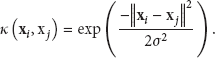
During actual application, there are three kinds of common kernel functions: polynomial kernel function, sigmoid kernel function, and Gaussian kernel function (also called radial basis kernel function) [19]. Of these, the Gaussian kernel function has the characteristic of maintaining the distance similarity of input function; this paper chooses the Gaussian kernel function to calculate the similarity between nodes, and its definition is as follows:

$$\begin{array}{cc}& \kappa \left({\mathbf{x}}_i,{\mathbf{x}}_j\right)=\exp \left(\frac{-{\parallel {\mathbf{x}}_i-{\mathbf{x}}_j\parallel }^{\mathrm{2}}}{\mathrm{2}{\sigma }^{\mathrm{2}}}\right).\end{array}$$

(4)

3.2. Kernel Sparsity Preserving Projections

First of all, KSPP uses the kernel method to map the data into a higher feature space, which makes it linearly separable in the higher feature space; then, it uses the SPP method to construct the adjacent matrix of sample data in the higher-dimensional feature space; finally, the adjacent matrix is used to conduct feature extraction through the graph embedding method.

Assume there is a set of training sample $\mathbf{X}=[x_{\mathrm{1}},x_{\mathrm{2}},\dots ,x_n]\in {\mathbb{R}}^{M\times n}$ ; firstly, use the nonlinear mapping function ϕ to map the training samples into a higher-d feature space to obtain $\Phi =[\varphi (x_{\mathrm{1}}),\varphi (x_{\mathrm{2}}),\dots ,\varphi (x_n)]$ , and then, similar to the SPP approach, use the improved ${\mathcal{l}}_{\mathrm{1}}$ optimization to reconstruct the feature space samples of each sample $\varphi ({\mathit{x}}_i)$ and obtain its corresponding weight coefficient ${\mathit{s}}_i$ . Therefore, the optimization problem can be expressed as

$$\begin{array}{l}\underset{s_i}{\min }\phantom{W}{\parallel {\mathit{s}}_i\parallel }_{\mathit{1}}\\ \text{s}.\text{t}.\phantom{\text{W}}\varphi \left(x_i\right)=\Phi {\mathit{s}}_i\\ \phantom{\text{s}.\text{t}.\text{W}}\mathbf{1}={\mathbf{1}}^T{\mathit{s}}_i,\end{array}$$

(5)

where ${\mathbf{s}}_i$ refers to the coefficient vector of SP in the feature space; $s_{ij}\hspace{0.17em}\hspace{0.17em}(j\ne i)$ refers to the contribution amount of the training sample $\varphi ({\mathit{x}}_j)$ to the reconstructed $\varphi ({\mathit{x}}_i)$ in the feature space. Similarly, higher-dimensional feature space also has noise, and in order to obtain the solution to the optimization, we need to relax restrictions on the optimization and obtain

$$\begin{array}{l}\underset{s_i}{\min }\phantom{W}{\parallel {\mathit{s}}_i\parallel }_{\mathit{1}}\\ \text{s}.\text{t}.\phantom{\text{W}}\parallel \varphi \left(x_i\right)-\Phi {\mathit{s}}_i\parallel \le \epsilon \\ \phantom{\text{s}.\text{t}.\text{W}}\mathrm{1}={\mathrm{1}}^T{\mathit{s}}_i.\end{array}$$

(6)

Because the mapping relation ϕ is unknown, Φ and the sample $\varphi ({\mathbf{x}}_i)$ in the higher feature space are also unknown, and therefore, the formula mentioned above cannot be directly solved. In accordance with (6), the optimization problem can be transformed to

$$\begin{array}{l}{\widehat{s}}_i=\underset{s_i}{\arg \hspace{0.17em}\min }{\parallel {\mathit{s}}_i\parallel }_{\mathit{1}}\\ \text{s}.\text{t}.\phantom{\text{W}}\parallel {\Phi }^T\Phi {\mathit{s}}_i-{\Phi }^T\varphi \left({\mathit{x}}_i\right)\parallel \le \epsilon \\ \phantom{\text{s}.\text{t}.\text{W}}\mathbf{1}=e^T{\mathit{s}}_i.\end{array}$$

(7)

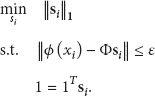
At this moment, the formula can be solved to obtain the estimated vector of SP coefficient, ${\widehat{s}}_i\hspace{0.17em}\hspace{0.17em}(i=\mathrm{1,2},\dots ,M)$ , and its combination is used to obtain the sparse reconstructed matrix $\mathbf{S}=[{\widehat{s}}_{\mathrm{1}},{\widehat{s}}_{\mathrm{2}},\dots ,{\widehat{s}}_M]$ . At this moment, the kernel SPP objective function is transformed to

$$\begin{array}{cc}& \underset{w}{\min }{\displaystyle \sum }_{i=\mathrm{1}}^M{\left({\mathbf{w}}^T\varphi \left(x_i\right)-{\mathbf{w}}^T\mathbf{B}{\widehat{\mathbf{s}}}_i\right)}^{\mathrm{2}}.\end{array}$$

(8)

Through deduction similar to SPP, we obtain the optimization criteria for KSPP; that is,

$$\begin{array}{cc}& \underset{w}{\min }\frac{{\mathbf{w}}^T\Phi \left(\mathbf{I}-\mathbf{S}-{\mathbf{S}}^T+\mathbf{S}{\mathbf{S}}^T\right){\Phi }^T\mathbf{w}}{{\mathbf{w}}^T\Phi {\Phi }^T\mathbf{w}}.\end{array}$$

(9)

Then, the criterion is transformed to a solution of the generalized characteristic equation:

$$\begin{array}{cc}& \Phi \left(\mathbf{S}+{\mathbf{S}}^T-\mathbf{S}{\mathbf{S}}^T\right){\Phi }^T\mathbf{w}=\lambda \Phi {\Phi }^T\mathbf{w}.\end{array}$$

(10)

Left-multiply ${\Phi }^T$ to the two sides of equation, and we obtain

$$\begin{array}{cc}& {\Phi }^T\Phi \left(\mathbf{S}+{\mathbf{S}}^T-\mathbf{S}{\mathbf{S}}^T\right){\Phi }^T\mathbf{w}=\lambda {\Phi }^T\Phi {\Phi }^T\mathbf{w}.\end{array}$$

(11)

w can be expressed as

$$\begin{array}{cc}& \mathbf{w}=\Phi p.\end{array}$$

(12)

The generalized characteristic equation can be simplified to

$$\begin{array}{cc}& K\left(\mathbf{S}+{\mathbf{S}}^T-\mathbf{S}{\mathbf{S}}^T\right)Kp=\lambda K^{\mathrm{2}}p.\end{array}$$

(13)

Solve the eigenvectors of the first d corresponding maximum eigenvalues $p_i\hspace{0.17em}\hspace{0.17em}(i=\mathrm{1,2},\dots ,d)$ .

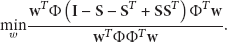
K is the inner product of data in the feature space calculated by kernel function; that is,

$$\begin{array}{l}{\Phi }^T\Phi ={\left[\varphi \left(x_{\mathrm{1}}\right),\varphi \left(x_{\mathrm{2}}\right),\dots ,\varphi \left(x_M\right)\right]}^T\\ \hspace{1em}\hspace{1em}\hspace{1em}·\left[\varphi \left(x_{\mathrm{1}}\right),\varphi \left(x_{\mathrm{2}}\right),\dots ,\varphi \left(x_M\right)\right]\\ \hspace{1em}\hspace{1em}=\left[\begin{array}{llll}K\left(x_{\mathrm{1}},x_{\mathrm{1}}\right)& K\left(x_{\mathrm{1}},x_{\mathrm{2}}\right)& \cdots & K\left(x_{\mathrm{1}},x_M\right)\\ K\left(x_{\mathrm{2}},x_{\mathrm{1}}\right)& K\left(x_{\mathrm{2}},x_{\mathrm{2}}\right)& \cdots & K\left(x_{\mathrm{2}},x_M\right)\\ ⋮& ⋮& \ddots & ⋮\\ K\left(x_M,x_{\mathrm{1}}\right)& K\left(x_M,x_{\mathrm{2}}\right)& \cdots & K\left(x_M,x_M\right)\end{array}\right]=K,\\ {\Phi }^T\varphi \left(x_i\right)={\left[\varphi \left(x_{\mathrm{1}}\right),\varphi \left(x_{\mathrm{2}}\right),\dots ,\varphi \left(x_M\right)\right]}^T\varphi \left(x_i\right)\\ \hspace{1em}\hspace{1em}=\left[\begin{array}{l}K\left(x_{\mathrm{1}},x_i\right)\\ K\left(x_{\mathrm{2}},x_i\right)\\ ⋮\\ K\left(x_M,x_i\right)\end{array}\right].\end{array}$$

(14)

After KSPP projection, the ith new eigenvector is

$$\begin{array}{l}{y}_i=w_i^T\phi \left(x\right)={\left(\frac{B{p}_i}{\sqrt{p_i^{T}K{p}_i}}\right)}^T\phi \left(x\right)=\frac{p_i^T{B}^T\phi \left(x\right)}{\sqrt{p_i^{T}K{p}_i}}\\ \hspace{1em}=\frac{p_i^T}{\sqrt{p_i^{T}K{p}_i}}\left[\begin{array}{l}K\left(x_{\mathrm{1}},x\right)\\ K\left(x_{\mathrm{2}},x\right)\\ ⋮\\ K\left(x_M,x\right)\end{array}\right].\end{array}$$

(15)

The total KSPP eigenvector is

$$\begin{array}{cc}& y=P^T\left[\begin{array}{c}K\left(x_{\mathrm{1}},x\right)\\ K\left(x_{\mathrm{2}},x\right)\\ ⋮\\ K\left(x_M,x\right)\end{array}\right].\end{array}$$

(16)

4. Localization Algorithm with KSPP

4.1. The Connection between Kernel Function and Localization

The localization algorithm based on kernel method uses a kernel function to map the RSSI vector between nodes into corresponding feature space. In this space, after a linear algorithm is used to calculate the relation between nodes, it is projected into the coordinate space; that is, through the kernel function, the RSSI vector $\mathit{S}\hspace{0.17em}\hspace{0.17em}(\mathit{S}=[{\mathit{s}}_1,{\mathit{s}}_2,\dots ,{\mathit{s}}_n])$ between n nodes in the monitoring area is related to the distance $\mathit{D}\hspace{0.17em}\hspace{0.17em}(\mathit{D}=[{\mathit{d}}_1,{\mathit{d}}_2,\dots ,{\mathit{d}}_n])$ between physical spaces, and Figure 3 shows this kind of relation.

In accordance with Figure 5, we can see that when the communication radiuses of two nodes have intersection, then direct communication can be conducted between these two nodes; the weaker the formed RSSI vector is when two nodes have received the RSSI signal of other nodes in the network, the farther the actual distance between them is, which means the less similar they are; the closer the distance between two nodes, the stronger the RSSI vector between them formed by other nodes in the area.

Figure 5

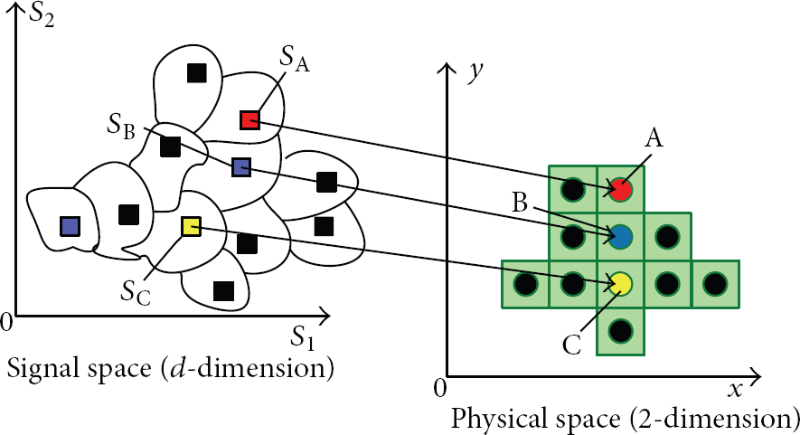
Correlation between the signal and physical location spaces.

In addition, in the literature [16], Pan proved that when the nodes are deployed in an idyllic environment, the RSSI matrix is positive semidefinite, so we can believe that the RSSI matrix itself is a kernel function matrix. Therefore, we can use the kernel method to measure the similarity between samples, which means the kernel function implicitly embeds the RSSI data into the feature space, and the linear algorithm is used in the feature space to solve the nonlinear relation of RSSI in the Euclidean space.

Assume in the monitoring area, n nodes generate n samples $\{{\mathit{x}}_1,{\mathit{x}}_2,\dots ,{\mathit{x}}_n\}$ , which are mapped into the feature space H through the kernel function $\kappa (·)$ ; then, H consists of set:

$$\begin{array}{cc}& \left\{\varphi \left({\mathit{x}}_1\right),\varphi \left({\mathit{x}}_2\right),\dots ,\varphi \left({\mathit{x}}_n\right)\right\}.\end{array}$$

(17)

Furthermore, the closer the nodes in the area are, the more similar the signal strength that they have received from other nodes is; therefore, we can believe the signal strength space and feature space H are related, and

$$\begin{array}{cc}& \varphi \left(·\right)=\left[s\left({\mathit{x}}_1,·\right),s\left({\mathit{x}}_2,·\right),\dots ,s\left({\mathit{x}}_n,·\right)\right],\end{array}$$

(18)

where $s({\mathit{x}}_i,{\mathit{x}}_j)$ refers to the value of RSSI received by node ${\mathit{x}}_i$ from node ${\mathit{x}}_j$ , and make $s({\mathit{x}}_i,{\mathit{x}}_i)=0$ ; the value of RSSI received by node ${\mathit{x}}_i$ from other nodes in the area is ${\mathit{s}}_i=[s({\mathit{x}}_i,{\mathit{x}}_1),s({\mathit{x}}_i,{\mathit{x}}_2),\dots ,s({\mathit{x}}_i,{\mathit{x}}_n){]}^T$ . Because Gaussian kernel function has the characteristic of maintaining the distance similarity of input space, this paper uses Gaussian kernel function for the calculation of similarity between nodes:

$$\begin{array}{l}\kappa \left({\mathbf{x}}_i,{\mathbf{x}}_j\right)=\exp \left(\frac{-{\parallel \varphi \left({\mathbf{x}}_i\right)-\varphi \left({\mathbf{x}}_j\right)\parallel }^{\mathrm{2}}}{\mathrm{2}{\sigma }^{\mathrm{2}}}\right)\\ \hspace{1em}\hspace{1em}\hspace{1em}=\exp \left(\frac{-{\sum }_{l=\mathrm{1}}^n{\left(s_{il}-s_{jl}\right)}^{\mathrm{2}}}{\mathrm{2}{\sigma }^{\mathrm{2}}}\right).\end{array}$$

(19)

The localization process of LE-KSPP proposed in this paper includes three steps: first of all, by using the collected RSSI values between nodes, the similarity between nodes is calculated through the Gaussian kernel function; secondly, the adjacency graph is automatically constructed through SP, which transforms the localization problem to dimensionality reduction problem on the graph; finally, the relative coordinates of all nodes in the monitoring area are estimated. The collected RSSI matrix between nodes and the Gaussian kernel function are utilized to construct the kernel function matrix; by solving (13), we can obtain the corresponding feature vector of maximum eigenvalue, and because the experiment was conducted in a two-dimensional space, only the first two biggest eigenvalues are used. Assume ${\lambda }_{\mathrm{1}},{\lambda }_{\mathrm{2}}$ are the first two biggest eigenvalues of (13), and ${\lambda }_{\mathrm{1}}\ge {\lambda }_{\mathrm{2}}$ ; their corresponding feature vectors are $p_{\mathrm{1}},p_{\mathrm{2}}$ . Through $p_{\mathrm{1}},p_{\mathrm{2}}$ , the base of the relative coordinate space between nodes can be indirectly determined, and make ${\widehat{\mathit{c}}}_i\in {\mathbb{R}}^2$ the estimated value of the relative coordinate of node ${\mathit{X}}_i$ . ${\widehat{\mathit{c}}}_i$ can be estimated through the following formula:

$$\begin{array}{cc}& {\widehat{\mathit{c}}}_i=\left[\begin{array}{c}{\widehat{c}}_{i1}\\ {\widehat{c}}_{i2}\end{array}\right]=\left[\begin{array}{c}{\displaystyle \sum }_{j=1}^N{p}_{1j}\kappa \left({\mathit{x}}_i,{\mathit{x}}_j\right)\\ {\displaystyle \sum }_{j=1}^N{p}_{2j}\kappa \left({\mathit{x}}_i,{\mathit{x}}_j\right)\end{array}\right],\end{array}$$

(20)

in which $p_{\mathrm{1}j}$ refers to the jth element of $p_{\mathrm{1}}$ and $p_{\mathrm{2}j}$ is the jth element of $p_{\mathrm{2}}$ .

The LE-KSPP algorithm can be utilized to obtain the relative location between nodes, but in most applications, the absolute coordinate of nodes should be obtained; therefore, the obtained relative coordinate should be transformed to absolute coordinate. If the system has provided adequate beacon nodes (in 2-dimensional space, at least three beacon nodes are required, and in 3-dimensional space, at least four beacon nodes are required), the relative coordinate of nodes can be transformed to absolute coordinate from relative to absolute. Assume the estimated absolute coordinate ${\widehat{\mathit{x}}}_i$ can be expressed by the following equation:

$$\begin{array}{cc}& {\widehat{\mathit{x}}}_i=\mathit{T}{\widehat{\mathit{c}}}_i+b.\end{array}$$

(21)

In other words, the absolute coordinate of the node is obtained through the transformation of coordinates, in which T is the transformation matrix and b is the offset, and its size can be determined by the beacon node.

Through deduction, we can obtain the estimated coordinate of unknown node is

$$\begin{array}{cc}& {\widehat{\mathit{x}}}_i=\mathit{T}\left({\widehat{\mathit{c}}}_i-{\widehat{\mathit{c}}}_b\right)+{\mathit{x}}_b,\hspace{1em}i=m+\mathrm{1},\dots ,n,\end{array}$$

(22)

where ${\mathit{c}}_b$ is the relative coordinate of any beacon nodes; ${\mathit{x}}_b$ is the corresponding absolute coordinate; the transformation matrix T can be obtained through the following equation:

$$\begin{array}{cc}& \mathit{T}=\Delta {\mathit{X}}_{-b}\Delta {\mathit{C}}_{-b}^T{\left(\Delta {\mathit{C}}_{-b}\Delta {\mathit{C}}_{-b}^T\right)}^{-1},\end{array}$$

(23)

where

$$\begin{array}{cc}& \Delta {\mathit{X}}_{-b}=\left[\Delta {\mathit{x}}_1,\dots ,\Delta {\mathit{x}}_{b-1},\Delta {\mathit{x}}_{b+1},\dots ,\Delta {\mathit{x}}_m\right],\\ \Delta {\mathit{C}}_{-b}=\left[\Delta {\mathit{c}}_1,\dots ,\Delta {\mathit{c}}_{b-1},\Delta {\mathit{c}}_{b+1},\dots ,\Delta {\mathit{c}}_m\right].\end{array}$$

(24)

While $\Delta {\mathit{x}}_i={\mathit{x}}_i-{\mathit{x}}_b$ , $\Delta {\mathit{c}}_i={\widehat{\mathit{c}}}_i-{\widehat{\mathit{c}}}_b$ . In order to avoid collinear or near collinear relation between beacon nodes, which might cause (23) to be unsolvable, we can use PCA to transform $\Delta {\mathit{C}}_{-b}$ and reduce the dimensionality of data, so that $\Delta {\mathit{C}}_{-b}\Delta {\mathit{C}}_{-b}^T$ is not singular any more. Therefore, before obtaining the transformation matrix T , first of all, conduct PCA transformation to $\Delta {\mathit{C}}_{-b}$ ; the projection matrix of PCA is recorded as P; then $\Delta {\mathit{C}}_{-b}^{\text{PCA}}={\mathit{P}}^T\Delta {\mathit{C}}_{-b}$ , so the expression of the transformation matrix ${\mathit{T}}^{\text{PCA}}$ is

$$\begin{array}{cc}& {\mathit{T}}^{\text{PCA}}=\Delta {\mathit{X}}_{-b}\mathit{P}{\left(\Delta {\mathit{C}}_{-b}^{\text{PCA}}\right)}^T{\left(\Delta {\mathit{C}}_{-b}^{\text{PCA}}{\left(\Delta {\mathit{C}}_{-b}^{\text{PCA}}\right)}^T\right)}^{-1}.\end{array}$$

(25)

At this moment, the absolute coordinate of unknown nodes can be obtained through the following formula:

$$\begin{array}{cc}& {\widehat{\mathit{x}}}_i={\mathit{T}}^{\text{PCA}}\left({\widehat{\mathit{c}}}_i-{\widehat{\mathit{c}}}_b\right)+{\mathit{x}}_b,\hspace{1em}i=m+1,\dots ,n.\end{array}$$

(26)

Consider there are n sensor nodes $X_1,X_2,\dots ,X_n$ deployed in area S; assume the first m nodes are beacon nodes $\{X_1,X_2,\dots ,X_m;m\ll n\}$ , the coordinates of beacon nodes are known, which are ${\mathbf{x}}_i$ , $i=1,\dots ,m$ , the rest $n-m$ nodes are unknown nodes, and their location information should be determined through certain localization algorithm.

About the LE-KSPP localization algorithm, see Algorithm 1, in which Steps (1) to (3) use the RSSI values between nodes to conduct training and learning; in Step (4), each node uses its adjacency relation with other nodes and estimates the relative coordinate of node through the training and learning model; by referring to the absolute location of beacon node, Step (5) transforms the node location of relative coordinate obtained in the area to absolute coordinate.

Algorithm 1: (LE-KSPP).

Input:

     Beacon node coordinate:

      $\left\{{\mathrm{x}}_{\mathrm{1}},{\mathrm{x}}_{\mathrm{2}},\dots ,{\mathrm{x}}_m\right\}$ , $m\ge \mathrm{3}$

     RSSI vector between nodes ${\left\{{\mathrm{s}}_i\right\}}_{i=\mathrm{1}}^n$

Output:

     Estimated coordinate of unknown

     nodes $\left\{{\widehat{\mathrm{x}}}_{m+\mathrm{1}},{\widehat{\mathrm{x}}}_{m+\mathrm{2}},\dots ,{\widehat{\mathrm{x}}}_n\right\}$ :

 (1) By using the collected RSSI vector

      between nodes ${\left\{s_{ij}\right\}}_{i,j=\mathrm{1}}^n$ , the similarity

      between nodes is calculated through

      Gaussian kernel function to form the kernel

      matrix K;

 (2) By solving the constrained optimization

      problem (See (6)), we obtain the kernel

      sparse representation coefficient

       ${\widehat{s}}_i(i=\mathrm{1,2},\dots ,M)$ , and use the ${\widehat{s}}_i$

      combination to obtain the kernel sparse

      reconstructed adjacent matrix;

 (3) Solve the optimal projection vector

       $p_{\mathrm{1}}$ , $p_{\mathrm{2}}$ , the two maximum eigenvalues

       ${\lambda }_{\mathrm{1}}$ , ${\lambda }_{\mathrm{2}}$ are obtained through the

      generalized characteristic equation

       $K(S+S^T-S{S}^T)Kp=\lambda K^{\mathrm{2}}p$ ,

      and their corresponding eigenvectors

       $p_{\mathrm{1}}$ , $p_{\mathrm{2}}$ are used as the optimal vectors;

 (4) Through (20), obtain the relative

      coordinate matrix;

 (5) Use the beacon nodes in the monitoring

      area, and transfer the relative coordinate

      into absolute coordinate; if the beacon

      nodes have a collinear or near collinear

      relation, adopt (26); if not, obtain the

      absolute coordinate $\left\{{\widehat{\mathrm{x}}}_{m+\mathrm{1}},{\widehat{\mathrm{x}}}_{m+\mathrm{2}},\dots ,{\widehat{\mathrm{x}}}_n\right\}$

      of unknown node through (22).

5. Simulation and Experiment

Consider a WSN which is comprised of n nodes $\{X_1,X_2,\dots ,X_n\}$ deployed in a $d\hspace{0.17em}\hspace{0.17em}(d=\mathrm{2,3})$ -dimensional monitoring area. The IDs of nodes are $\mathrm{1,2},\dots ,n$ , respectively, the actual coordinate of node $X_i$ is ${\mathit{x}}_i$ , and $\mathit{X}={[{\mathit{x}}_1,{\mathit{x}}_2,\dots ,{\mathit{x}}_n]}^T$ represents the coordinate matrix of node. Without loss of generality, let the first $m\hspace{0.17em}\hspace{0.17em}(m\ll n)$ nodes in the n nodes be as beacon nodes, and make ${\mathit{X}}_b=[{\mathit{x}}_1,{\mathit{x}}_2,\dots ,{\mathit{x}}_m{]}^T$ represent the coordinate matrix of beacon nodes. The purpose of localization method is to estimate the values of unknown nodes coordinate ${\widehat{\mathit{x}}}_i\hspace{0.17em}\hspace{0.17em}(i=m+1,m+2,\dots ,n)$ , which makes the estimated coordinate ${\widehat{\mathit{x}}}_i$ as close to the actual coordinate ${\mathit{x}}_i$ of unknown nodes as possible.

Related literature [20] points out that the received signal strength s between nodes has a certain proportional relation with their distance d. In an ideal environment, node i is within the communication radius of node j, and the signal strength and distance have the following relation:

$$\begin{array}{cc}& s\left(X_i,X_j\right)=kPd{\left(X_i,X_j\right)}^{-\mu },\end{array}$$

(27)

where P is the sending signal voltage, k is the proportionality coefficient, μ is the signal attenuation coefficient, usually $\mu >\mathrm{2}$ , and $d(X_i,X_j)$ is the actual distance between node i and node j. If node i is not within the communication radius of node j, we denote $s(X_i,X_j)=0$ .

This section analyzes and assesses the performance of LE-KSPP localization method through experiment and simulation. In the experiment, the nodes were assigned in a two-dimensional space, and measurement of the distance between nodes adopted the range model-based simulation experiment and actual measurement-based data set, respectively. The parameters involved in the range model are fit with the values collected by Patwari [32], and the actual measurement data set is the RSSI data collected by Patwari experiment team [33] in a $\mathrm{12}\hspace{0.17em}\text{m}\times \mathrm{14}\hspace{0.17em}\text{m}$ rectangular area. For the experiment of range model-based, the nodes are randomly or regularly deployed in the monitoring area. In order to investigate whether the algorithm is affected by the obstacle, a blocking experiment was added to the two deployment strategies mentioned above; that is, assume a big blocking object was put in the deployment area to make communication impossible between nodes, and this kind of area has a C sharp. For different network topology structures, by redeploying nodes in the same area for multiple times, all of the reported results are the average over 100 trials. The data set was actually measured through 44 nodes (including 4 beacon nodes) in the monitoring area, the center frequency of node was 2.4 Hz, the broadband direct sequence was used for spread spectrum communication, each RSSI value was measured for 10 times, and each node received and sent for 5 times.

Because it is difficult to evaluate performance by using relative coordinate, we adopted absolute coordinate to express location of nodes in this experiment. We also compare our LE-KSPP algorithm, which is built on one kind of graph embedding localization, with the same kind of algorithms such as MDS-MAP [34], Isomap [35], and LE-KLPP [18]. In addition, the location accuracy of ours and KLPP are both related to kernel function, which is called Gauss kernel function in our selection. We also found there is a certain relationship between kernel parameter σ and the distance between training samples, so in the experiment we assume the average distance between sample nodes of σ (4) as 50 times, and the cumulative variance contribution rate of PCA as 90%.

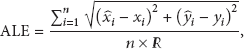
The paper utilizes Average Localization Error (ALE) performance index to evaluate the performance of the algorithm. The formula is shown as follows:

$$\begin{array}{cc}& \text{ALE}=\frac{{\sum }_{i=1}^n\sqrt{{\left({\widehat{x}}_i-x_i\right)}^2+{\left({\widehat{y}}_i-y_i\right)}^2}}{n\times R},\end{array}$$

(28)

where n is the number of unknown nodes, $(x_i,y_i)$ is the unknown node actual location, $({\widehat{x}}_i,{\widehat{y}}_i)$ is unknown node evaluated location, and R is the radio range of sensor nodes.

5.1. Localization Results with Range Model-Based

In order to compare the impartiality of the experimental results, when the measurement information is based on signal strength model, in this section, the signal model in literature [32, 33] is used to simulate the signal strength between the nodes:

$$\begin{array}{l}{P}_{ij}~N\left({\stackrel{-}{P}}_{ij},{\sigma }_{\text{dB}}^2\right),\\ {\stackrel{-}{P}}_{ij}=P_0-10n_p\text{lg}\phantom{1}\left(\frac{d_{ij}}{d_0}\right),\end{array}$$

(29)

among which $P_{ij}$ represents the transmitted signal power which is received by node i from node j, and the unit is dBm; $P_0$ represents the received signal power corresponding to the point of the reference range $d_0$ ; $d_0$ represents the reference range; $n_p$ represents the attenuation coefficient of the wireless transmission, related to the environment; ${\stackrel{-}{P}}_{ij}$ represents the received signal power corresponding to the point of the reference range $d_0$ (dBm); ${\sigma }_{\text{dB}}^{\mathrm{2}}$ represents the shadow variance.

Among these, $n_p$ uses the data in the literature, but ${\sigma }_{\text{dB}}^2/n_p=1.7$ .

5.1.1. Regular Deployment

In this group of experiments, the nodes were regularly deployed in a $\mathrm{200}\hspace{0.17em}\text{m}\times \mathrm{200}\hspace{0.17em}\text{m}$ area, in which the grid has a side length of 10 m. Under the unblocked situation, there were 441 nodes in total; under the blocked situation, the number of nodes was changed to 381; 5 to 15 nodes were chosen as the beacon nodes, which were assured that their location information was known.

Before analyzing performance of LE-KSPP algorithm, let us first investigate the two final localization results under different deployment. In Figure 6, the circles denote the unknown node and the squares are the beacon, the line connects the actual coordinate and estimated coordinate of unknown nodes, and the longer the line is, the more the estimated value deviates from the actual location. Figure 6 indicates the localization results for each node under regular deployment with 10 beacons. The LE-KSPP algorithm of ALE for this uniformly deployed network is about 14.9% (Figure 6(a)) and 19.9% (Figure 6(b)).

Figure 6

Localization result with 10 beacons under regular deployment.

Figure 7 describes the impact of the beacon nodes number (from 5 to 15) on the ALE of the two localization algorithms of four localization algorithms in a regularly deployed network. They are regularly deployed in two blocked and unblocked environments, respectively. We can note that our algorithm always obtains the best results. Different with the MDS-MAP, Isomap and LE-KLPP, the localization accuracy of our algorithm raises with the increase of beacon nodes. This is because LE-KSPP method can reconstruct the relation between nodes through SP, and opposed to other methods, it can more self-adaptively choose and decide the node number and weight around its location.

Figure 7

ALE with different number of beacons.

5.1.2. Random Deployment

In this group of experiments, 200 nodes were randomly deployed in a $\mathrm{200}\hspace{0.17em}\text{m}\times \mathrm{200}\hspace{0.17em}\text{m}$ two-dimensional square area, and 5 to 15 nodes were chosen from the 200 as the beacon nodes. Like the regular deployment, in order to investigate the influence of non-line-of-sight on the localization algorithm, the experiment scenario with obstacle was added to the random deployment experiment, and in addition, the signal strength between nodes was still simulated by using (29).

Similarly, the two definitive localization results were analyzed first. As showed in Figure 8, in these two experiments, the number of beacon nodes is still 10. Under the unblocked situation, LE-KSPP is about 17.5%; the corresponding ALE is 24.6% under the blocked situation.

Figure 8

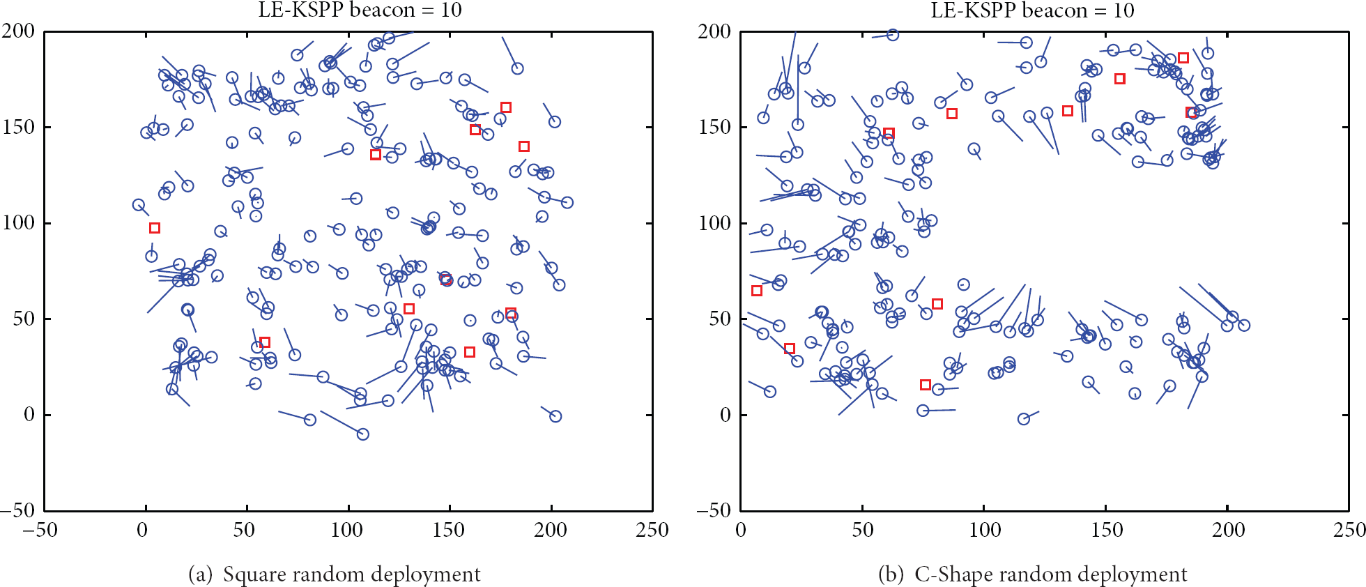
Localization result with 10 beacons under random deployment.

In Figure 9, for the randomly placed sensor network, we also compare it with the other algorithms (i.e., MDS-MAP, Isomap, and LE-KLPP) under different number of beacons. We can see that our algorithm always achieves the minimal average location error. When the number of beacons is 5 and 7, the ALE of value of MDS-MAP and LE-KLPP is even bigger than 40%, respectively.

Figure 9

ALE with different number of beacons.

5.2. Localization Results with the Actually Measured Data Sets

The literature and experiment of Section 5.1 show that the LE-KLPP has a better performance than the MDS-MAP and Isomap algorithm; therefore, only LE-KSPP algorithm and LE-KLPP algorithm are compared in this group experiment. The experimental data come from the SPAN lab, and the experimental scenario is as shown in Figure 10.

Figure 10

Actual collection area.

By using the data set mentioned above, this paper has compared the localization performance of the LE-KLPP and LE-KSPP algorithms, and see Table 1 for the experiment results. In accordance with Table 1, we can see that under separate communication radius (CR), the localization accuracies of LE-KSPP are all higher than the LE-KLPP algorithm, and the ALE has an increase of more than 10%.

Table 1

The ALE of LE-KLPP and LE-KSPP with actual RSSI-based ranging.

CR (m)	The ALE of LE-KLPP	The ALE of LE-KSPP
6.5	23.71%	17.24%
7	15.68%	14.11%
7.5	14.04%	11.73%
8	12.66%	10.46%

Figure 11 shows the localization result under the communication radius of 7.5 m. In the figure, we can see that the closer these two algorithms are to the beacon node point, the smaller the estimated error is, which means, because the beacon node has an accurate location, it is more accurate to use it to determine the location of unknown node; in Figure 11, the LE-KLPP algorithm is used, because it artificially sets parameter k and it causes that an optimal solution (short line) can be obtained in certain area (far from the beacon node), while in some area, it does not apply (long line); in Figure 11, the LE-KSPP algorithm is chosen, because SP is used to self-adaptively obtain the number of adjacent points and the obtained estimation value is relatively stable (the length of line does not have big change).

Figure 11

Location estimates with actual RSSI-based ranging.

6. Conclusion

This paper studies the localization problem of sensor network nodes built on signal strength, and the LE-KSPP algorithm is proposed. This LE-KSPP utilizes the kernel method to map the signal strength to a higher-dimensional feature space and conducts SP, and then, the SP coefficient of the obtained signal set is obtained through SP. Because the data in a higher-dimensional feature space have better linear separability, the SP can self-adaptively capture the “local” structure of data, and different sample points are automatically endowed with different “adjacency” number and parameter selection is avoided, which makes the algorithm more applicable to different environments.

The experiments in this paper show that the proposed LE-KSPP algorithm can obtain relatively satisfying localization results on both range model and actually measured data, the impact of the beacon nodes number and blockage on this algorithm is small, and it can self-adapt to various network topology environments, which has a high robustness.