Optimal Deployment and Scheduling with Directional Sensors for Energy-Efficient Barrier Coverage

Abstract

In recent years, barrier coverage problem in directional sensor networks has been an interesting research issue. Most of the existing solutions to this problem aim to find as many barrier sets as possible to enhance coverage for the target area, which did not consider the power conservation. In this paper, we address the efficient sensor deployment (ESD) problem and energy-efficient barrier coverage (EEBC) problem for directional sensor networks. First, we describe a deployment model for the distribution of sensor locations to analyze whether a target area can be barrier covered. By this model, we examine the relationship between the probability of barrier coverage and network deployment parameters. Moreover, we model the EEBC as an optimization problem. An efficient scheduling algorithm is proposed to prolong the network lifetime when the target area is barrier covered. Simulation results are presented to demonstrate the performance of this algorithm.

1. Introduction

Directional sensors, such as image sensors [1], video sensors [2] and infrared sensors [3], have been widely used to improve the performance of wireless sensor networks. Directional sensor has a limited angle of sensing range due to the technical constraints or cost considerations, which is different from omnidirectional sensor. Directional sensors may have several working directions and adjust their sensing directions during their operation.

Power conservation is another important issue for directional sensor, just like omnidirectional sensor. Power consumption of sensor nodes has a great impact on the lifetime of sensor networks. Most directional sensors have limited power sources which are supplied by batteries. The batteries of sensors are not rechargeable due to the hostile or inaccessible environments in many scenarios. Due to the small size of existing batteries, sensor nodes cannot last as long as desired.

Barrier coverage is an efficient way for many applications in directional sensor networks (DSNs), such as intrusion detection and border surveillance [4, 5]. There are two kinds of barrier coverage, that is, weak and strong [6], which are illustrated in Figure 1. Weak barrier coverage guarantees detections of intruders moving along congruent crossing paths, but it does not guarantee the detection of intruders moving along arbitrary crossing paths. Strong barrier coverage guarantees that no intruders can cross the region undetected no matter what crossing paths they choose. Constructing a strong barrier with directional sensors for a target region is a challenging problem. In this paper, we will focus on strong barrier coverage for DSNs. For convenience, this paper will use barrier coverage to refer to strong barrier coverage.

Figure 1

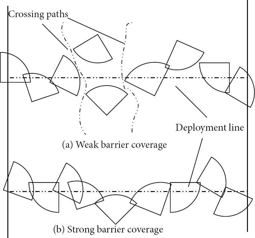
Strong and weak barrier coverage for DSNs.

In this work, we separate barrier coverage problem for DSNs into two subproblems, that is, $(1)$ whether a target area can be barrier covered by the directional sensors and $(2)$ how long a target area can be barrier covered.

On the one hand, whether a target area can be barrier covered is affected by sensor deployment methods. In certain applications, for example, indoor application, sensors are placed with desired locations. In other cases, such as remote or inhospitable environments, sensors are deployed randomly by airplanes. In determined placement, we need to minimize the number of sensors by optimizing their locations to form a barrier. In random placement, barrier coverage depends on the distribution of sensor locations. Besides, network parameters, such as the number of nodes, the sensing radius of each sensor, and the number of directions per sensor, have important effects on the probability of barrier coverage.

On the other hand, how long a target can be barrier covered is affected by scheduling algorithm with directional sensors. We call a subset of directions of the sensors in which the directions achieve a barrier for the target area as a barrier set. Directional sensor has multiple working directions, but different directions of the same sensor cannot work at the same time. So there is no more than one direction from the same sensor in a barrier set. We may find multiple barrier sets for a directional sensor network. The work time of each barrier set is limited to the remaining work time of sensor in the barrier set. Directional sensor will die when its power is exhausted. To conserve energy, we make different barrier sets work at different times. We leave the necessary sensors which are in a working barrier set in the active state and put other sensors into sleep state. So the target area can be barrier covered continuously by the barrier sets. The network lifetime is the total work time of the barrier sets.

In this paper, we study the energy-efficient barrier coverage problem for directional sensor networks. We consider the following scenario. The target area is a two-dimensional Euclidean plane. A number of directional sensors are deployed side by side along straight line across the region by airplane. After they have been deployed, they will never move. We first describe the sensing model of each sensor and then define ESD and EEBC problems we need to solve. Our contributions are as follows. First, we describe a deployment model for the distribution of sensor locations to solve the ESD problem. We analyze the overlap conditions of the neighboring sensors, and get a function to compute the probability of barrier coverage with some parameters. Then the relationships between the probability of the barrier coverage and network parameters are studied in different deployment scenarios. Our results investigate that the probability of barrier coverage is more sensitive to a number of sensors and sensing radius of each sensor. Second, we propose an energy-efficient scheduling algorithm to prolong the network lifetime when the target area is barrier covered. We model the EEBC as an optimization problem. We introduce a directed graph to model the overlap of directional sensors. Based on this graph, we describe an integer linear programming formulation to find out barrier sets in the network. By solving the optimization problem, we get the optimal solutions, the barrier sets, and their work times. These barrier sets work continuously with their work times to maximize the network lifetime.

The remainder of this paper is organized as follows. In Section 2, we briefly survey the related work on barrier coverage of sensor networks. In Section 3, we define the ESD and EEBC problems. In Section 4, we propose and evaluate a solution to the ESD. In Section 5, we present an energy-efficient algorithm to solve the EEBC and give the simulation results for the EEBC. Finally, we conclude this paper in Section 6.

2. Related Work

In the past years, the barrier coverage problem in wireless sensor networks has been fairly well studied in the literature.

Sensor deployment strategies have direct impact on the barrier coverage of wireless sensor networks. Different deployment strategies can result in significantly different barrier coverage. Kumar et al. [7] defined the notion of barrier coverage of a belt region using wireless sensors. They proposed efficient algorithm to determine whether a region is barrier covered or not after deployment. Then they established the optimal deployment pattern for achieving barrier coverage. In [8], Saipulla et al. established a tight lower bound for the existence of barrier coverage under line-based deployment. Their results provided important guidelines to the deployment and performance of wireless sensor networks for barrier coverage. Balister et al. [9] computed the probability that the nodes provide barrier coverage when they are deployed by the Poisson point process.

Most of the barrier coverage literatures assumed that every sensor node is stationary in the sensor networks. Zhang et al. [10] studied a strong barrier coverage problem for DSNs. They presented an integer linear programming formulation for the problem. Then several efficient centralized algorithms and a distributed algorithm were proposed to solve the problem. Wang and Cao [11] considered the problem of constructing camera barrier in both random and deterministic deployment. They proposed a novel method to select camera sensors to form a camera barrier, which is essentially a connected zone across the monitored field such that every point within this zone is full view covered. In [12], Chen et al. introduced the concept of local barrier coverage and showed that local barrier coverage almost always provides global barrier coverage for thin belt regions. They also developed a novel sleep-wake-up algorithm to maximize network lifetime. Liu et al. [6] believed quality of barrier coverage is not binary. They proposed a metric for measuring the quality of k-barrier coverage and established theorems that can be used to precisely measure the quality using the proposed metric. In [13], Chen et al. provided theoretical foundations for the construction of strong barriers in a sensor network. They obtained the critical conditions for strong barrier coverage in a strip sensor network. Based on this result, they further proposed an efficient distributed algorithm.

There are some literatures which focus on barrier coverage for sensor networks with mobile sensors. Saipulla et al. [14] studied the barrier coverage with mobile sensors of limited mobility. They first explored the fundamental limits of sensor mobility on barrier coverage and presented a sensor mobility scheme that constructs the maximum number of barriers with minimum sensor moving distance. They further devised an algorithm that computes the existence of barrier coverage under the limited sensor mobility constraint and constructed a barrier if it exits. In [15], He et al. considered the barrier coverage problem where m sensors are needed to guarantee full barrier coverage and there are only n mobile sensors available ( $n<m$ ). They first modeled the arrival of intruders at a specific location as a renew process. Then they proposed two sensor patrolling algorithms to solve the problem: periodical monitoring scheduling (PMS) and coordinated sensor patrolling (CSP). In [16], Keung et al. demonstrated the intrusion detection problem as a classical kinetic theory of gas molecules in physics. By examining the correlations and sensitivity from the system parameters, they derived the minimum number of mobile sensors that needs to be deployed in order to maintain the k-barrier coverage for a mobile sensor network.

Most of existing solutions to barrier coverage problem aim to find as many barrier sets as possible to enhance coverage for the target area. However, power conservation is still an important issue in directional sensor networks. Therefore, in this paper, we will study the energy-efficient barrier coverage problem with directional sensors.

3. Problem Statement

In this section, we give the assumptions and formally define the problems we need to solve, followed by a simple example of the EEBC to briefly describe this problem.

3.1. Assumptions and Problem Definition

In this paper, we consider the following scenario. The target region is a belt region, which is like a two-dimensional rectangular area. Sensors are deployed in the area along the deployment line (as shown in Figure 1) by airplane. After sensors have been deployed, they will never move. We assume that all the sensors have the same sensing radius and angle of view. The size of the angle of view may theoretically change from 0 to 2*pi. So each sensor has multiple working directions, and sensing region of each working direction is a sector. Different directions of the same sensor do not overlap. No more than one direction of each sensor can be active at the same time.

We adopt some notations throughout the paper. Let L and W be the length and the width of the target area, respectively. $S_i$ denotes the ith sensor in the network. R denotes the sensing radius of each sensor. We define M as the number of directions of each sensor. $b_{i,j}$ ( $i=1,\dots ,N,j=1,\dots ,M$ ) denotes the jth direction of ith sensor. Each sensor initially has an equal lifetime, which is defined as T.

Figure 2 is an example to illustrate the sensing model of directional sensor in this paper. The angel of view of sensor $S_i$ is pi/2. So $S_i$ have four directions: $b_{i,1}$ , $b_{i,2}$ , $b_{i,3}$ , and $b_{i,4}$ (as shown in Figure 2). Intruder-1 can be detected by the direction $b_{i,3}$ if it satisfies the two following conditions:

$$\begin{array}{cc}& \left|\overrightarrow{Q}\right|\le R,\end{array}$$

(1)

$$\begin{array}{cc}& \overrightarrow{G}·\overrightarrow{Q}\mathrm{\hspace{0.17em}\hspace{0.17em}}\ge \left|\overrightarrow{Q}\right|\cos \frac{\alpha }{\mathrm{2}}.\end{array}$$

(2)

Figure 2

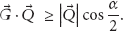
Sensing model of a directional sensor.

Conditions (1) and (2) mean that the intruder is detected by a sensor if it is located anywhere within the active working direction of the sensor. As shown in Figure 2, intruder-1 can be detected by $b_{i,3}$ . However, intruder-2 cannot be detected by any direction of $S_i$ .

We provide the following problem definitions.

Definition 1 (ESD (efficient sensor deploy) problem).

For a given target area (length L, width W), find out the relationships between the probability of barrier coverage and the deployment parameters: number of nodes (N), sensing radius of each sensor (R), and the number of directions of each sensor (M).

Definition 2 (EEBC (energy-efficient barrier coverage) problem).

Find a family of K barrier sets $B_1,B_2,B_3,\dots ,B_k$ , with nonnegative work time $t_1,t_2,\dots ,t_k$ , such that $t_1+t_2+\cdots +t_k$ is maximized, and for each sensor, the total work time is less than the initial lifetime (T).

3.2. Example for EEBC

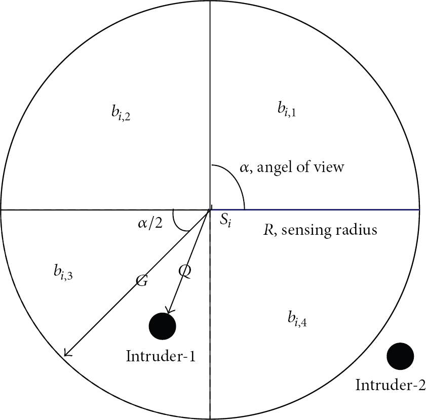
Figure 3 shows a directional sensor network with three sensors ( $S_1$ , $S_2$ , and $S_3$ ) deployed to detect the intruders who want to cross the belt region. Each sensor has an initial lifetime of 1 (time unit). Each sensor has four working directions (illustrated in Figure 3). For example, $\{b_{\mathrm{1,4}},b_{2,2}\}$ is a barrier set for the network. We can find out multiple barrier sets for this network. If we set any barrier set with the work time of 1, the network lifetime is 1. On the other hand, we can get the following barrier sets: $B_1=\{b_{1,1},b_{2,2}\}$ with the work time of 0.5, $B_2=\{b_{\mathrm{1,4}},b_{\mathrm{3,1}}\}$ with 0.5, and $B_3=\{b_{3,2},b_{2,3}\}$ with 0.5. The total work time of each sensor is no more than 1. Finally, the network lifetime is maximized to 1.5. This implies that efficient scheduling can prolong the lifetime of the network.

Figure 3

Example of EEBC.

4. Deployment Model and Analysis

In this section, we will solve the ESD problem.

4.1. Deployment Model for DSNs

In this section, we introduce a deployment model for directional sensor networks in this work.

Suppose that N sensors are deployed by the deployment line evenly from the left to the right. We get the location of each sensor. The coordinates $(x_i,y_i)$ of the ith sensor $S_i$ are:

$$\begin{array}{cc}& x_i=i*\frac{L}{\left(N+\mathrm{1}\right)}+{\gamma }_{i\mathrm{\hspace{0.17em}\hspace{0.17em}}},\hspace{1em}i=\mathrm{1,2},\dots ,N,\end{array}$$

(3)

$$\begin{array}{cc}& y_i={\tau }_i,\hspace{1em}i=\mathrm{1,2},\dots ,N.\end{array}$$

(4)

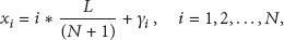
Because of mechanical inaccuracy, terrain constraints, wind, and other environmental factors, the sensors cannot be deployed with the location we desired. Therefore, ${\gamma }_i$ and ${\tau }_i$ denote the offset of the ith sensor in the horizontal and vertical directions, respectively. And in this model, we assume that the random offsets ${\gamma }_i$ and ${\tau }_i$ are independently and identically distributed with a normal distribution of zero mean and δ variance.

In this paper, each directional sensor has different working directions and can detect any intruder within its active direction. And a barrier set is formed by overlapped directions that intersect both the left and right boundaries of the target area. Such a barrier set can guarantee that no intruders can cross the target area without being detected. We consider the following cases to find out the overlap conditions of neighboring sensors, that is, $S_1$ and $S_2$ (as shown in Figure 4). Each sensor in this figure has four directions. We define $d\hspace{0.17em}\hspace{0.17em}(d=|S_2-S_1|)$ as the distance between the two neighboring sensors, $S_1$ and $S_2$ .

Figure 4

Overlap conditions of neighboring sensors.

Case  1. Figure 4(a) shows the distance between $S_1$ and $S_2$ that is no more than R. In this condition, we can see that $b_{\mathrm{2,3}}$ can overlap any direction of $S_1$ and also $b_{1,1}$ can overlap any direction of $S_2$ . This means that, no matter which direction of $S_1$ is active, $S_2$ can find a direction to be active to overlap $S_1$ .

Case  2. Figure 4(b) shows the distance between $S_1$ and $S_2$ that is more than R but less than $2R$ . In this condition, there are some directions of these two sensors that can overlap each other, like $b_{\mathrm{1,1}}$ and $b_{\mathrm{2,2}}$ . However, there exist some directions, which none directions of the other sensor can overlap. For example, if $b_{1,2}$ is active, none of directions of $S_2$ can overlap it.

Case  3. Figure 4(c) shows the distance between $S_1$ and $S_2$ that is more than $2R$ . In this condition, we cannot find any direction from $S_1$ to overlap the direction from $S_2$ .

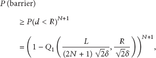
Theorem 3.

When N directional sensors are deployed from the left to the right in a target area with the coordinates ( $x_i,y_i$ ) and the sensing radius R, the probability of the target area can be barrier covered by these sensors given by

$$\begin{array}{cc}& P\left(\text{barrier}\right)\mathrm{\hspace{0.17em}\hspace{0.17em}}\ge P\left(d_{\mathrm{0}}<R\right)P\left(d_N<R\right)\prod _{i=\mathrm{1}}^{N-\mathrm{1}}P\left(d_i<R\right),\end{array}$$

(5)

where $d_0$ is the distance between the sensor $S_1$ and the left boundary. $d_N$ is the distance between the sensor $S_N$ and the right boundary. $d_i$ is the distance between $S_{i+1}$ and $S_i$ .

Proof.

There are N sensors with the following conditions. $(1)$    $d_0<R$ , which means the left boundary can be covered by the sensor. $(2)$      $d_i<R$ , which means the neighboring sensors could overlap each other. $(3)$      $d_N<R$ , which means the right boundary can be barrier covered. When they satisfy these three conditions, the sensors can form a barrier for the target area. These three conditions are a sufficient condition for barrier coverage with directional sensors. Hence, the theorem holds.

We can get

$$\begin{array}{cc}& d_i=\left|S_{i+\mathrm{1}}-S_i\right|=\frac{L}{N+1}+\left({\gamma }_{i+1}-{\gamma }_i\right)+{\tau }_{i+1}-{\tau }_i.\end{array}$$

(6)

Formulation (6) implies that $d_i$ follows a Ricean distribution [14]. Also, we can easily verify that $P(d_0<R)>P(d_i<R)$ and $P(d_N<R)>P(d_i<R)$ . Therefore, we denote d as the distance between neighboring sensors. We get

$$\begin{array}{l}P\left(\text{barrier}\right)\\ \hspace{1em}\hspace{1em}\ge P{\left(d<R\right)}^{N+\mathrm{1}}\\ \hspace{1em}\hspace{1em}={\left(\mathrm{1}-Q_{\mathrm{1}}\left(\frac{L}{\left(\mathrm{2}N+\mathrm{1}\right)\sqrt{\mathrm{2}}\delta },\frac{R}{\sqrt{\mathrm{2}}\delta }\right)\right)}^{N+\mathrm{1}},\end{array}$$

(7)

where $Q_1$ is Marcum's Q-function of the first order. By formulation (7), we can make a rough calculation of the barrier coverage probability for a directional sensor network with given parameters.

4.2. Model Analysis and Simulation Results

In this section, we compare our model analysis described in Section 4.1 and simulation results in different scenarios. We study the relationships between the barrier coverage probability and the network parameters, such as the number of sensors (N), sensing radius of each sensor (R), and the number of directions of each sensor (M).

Figure 5 plots the relationship between the probability of barrier coverage and the number of sensors (N) when $L=2000$  m, $R=60$  m, and $M=4$ . Figure 6 plots the relationship between the probability of barrier coverage and sensing radius (R) when $L=2000$  m, $N=40$ , and $M=4$ . In these two figures, we consider three different variances $\delta =8$ , 6, and 4. Figure 7 plots the probability of barrier coverage when M values 3, 4, 6, and 12. In this figure, $L=2000$  m, $N=40$ , $R=65$  m, and $\delta =4$ .

Figure 5

Barrier coverage probability versus N, when $L=2000$  m, $R=60$  m, $M=4$ .

Figure 6

Barrier coverage probability versus R, when $L=2000$  m, $N=40$ , and $M=4$ .

Figure 7

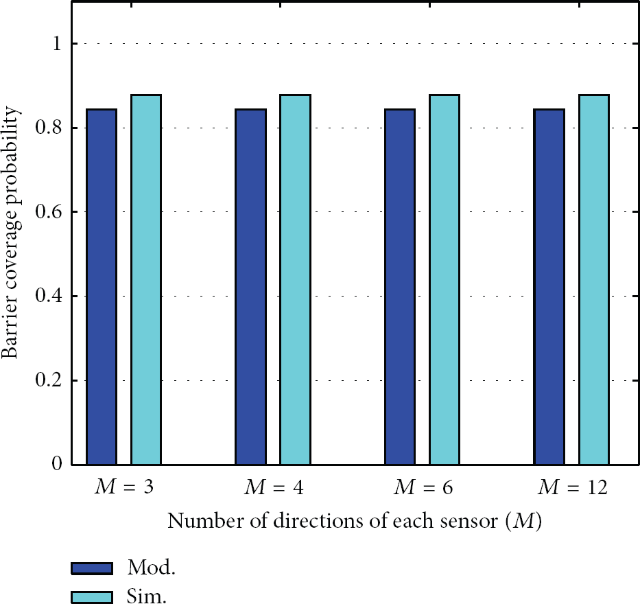
Barrier coverage probability versus M, when $L=2000$  m, $N=40$ , $R=65$  m, and $\delta =4$ .

As shown in Figures 5, 6, and 7, there is a good match between our model analysis and simulation results. The match improves as the variance δ decreases. Also we can verify that our model analysis is indeed a lower bound than the simulation results.

In Figures 5 and 6, we can see that the probability of barrier coverage increases monotonically as the number of sensors $(N)$ and the sensing radius $(R)$ increase. The reason is that when the number of sensors increases, the distance between neighboring sensors will decrease, which leads to the more probability of barrier coverage. When the sensing radius increases, each direction can overlap more other directions. Therefore, the network has more probability to form a barrier. However, Figure 7 implies that the number of directions of each sensor has an effect on the probability of barrier coverage both in our analysis and simulation results.

We can observe from the results above that increasing the number of nodes or sensing radius is an efficient way to improve the probability of barrier coverage. And our analysis can guide the deployment methods and parameters in the realistic application.

5. Energy-Efficient Barrier Coverage

This section focuses on the EEBC problem. By the deployment model and analysis in Section 4, we get several methods to improve the probability of barrier coverage. Next, we discuss how to schedule directional sensors in the network to form energy-efficient barriers.

5.1. Optimization Formulation for EEBC

In this section, we model optimization formulation for EEBC problem. In the EEBC problem, we wish to compute the value L which is the longest lifetime of the network, where the network lifetime is defined as the time duration when the target area is barrier covered by a set of active directions of different sensors. The lifetime of a network is limited by the remaining energy of single sensor which works in the network. When one of the working sensors runs out of energy, the barrier set which it belongs to cannot work.

We assume that N sensors are deployed in a target area to form barriers. The network can find K barrier sets by some algorithm. The kth barrier set is denoted by $B_k$ , which is formed of $b_{i,j}\hspace{0.17em}\hspace{0.17em}(i=1,\dots ,N,j=1,\dots ,M)$ . $t_k$ denotes the work time of $B_k$ . We set a Boolean variable $C_{i,j,k}$ as

$$\begin{array}{cc}& C_{i,j,k}=\{\begin{array}{cc}\mathrm{1},\hfill & b_{i,j}\in B_k\hfill \\ \mathrm{0},\hfill & \text{otherwise}.\hfill \end{array}\end{array}$$

(8)

Thus, we obtain the following optimization formulation to compute the maximum lifetime of the network:

$$\begin{array}{cc}& \text{maximize}\hspace{1em}L=t_1+t_2+t_3+\cdots +t_k\end{array}$$

(9)

subject to

$$\begin{array}{cc}& \sum _{j=1}^M\hspace{0.17em}\sum _{k=1}^K{C}_{i,j,k}{t}_k\le T,\hspace{1em}i=\mathrm{1,2},\dots ,N\end{array}$$

(10)

$$\begin{array}{cc}& \sum _{j=1}^M{C}_{i,j,k}\le 1,\hspace{1em}i=\mathrm{1,2},\dots ,N,\hspace{0.17em}\hspace{0.17em}k=\mathrm{1,2},\dots ,K\end{array}$$

(11)

$$\begin{array}{cc}& C_{i,j,k}=\left\{\mathrm{0,1}\right\},\hspace{1em}{t}_k\ge 0.\end{array}$$

(12)

The objective function (9) maximizes the lifetime of the network. The maximum lifetime is the work time of the network, which meets the constraints (10)–(12) and maximizes the lifetime value. It is the total work time of K barrier sets.

The constraint (10) indicates that each barrier set cannot contain different directions which belonging to the same sensor. No more than one direction of the same sensor can work at the same time. The constraint (11) shows the lifetime constraint for each sensor. The total work time of the M directions belong to the same sensor is no more than the initial lifetime of the sensor. The constraint (12) shows the restrictions on the variables. The variable $C_{i,j,k}$ can be either 1 or 0, which means the direction $b_{i,j}$ works either in the kth barrier or not. The work time $t_k$ cannot be negative.

This optimization formulation is a mixed integer programming problem. If we find the barrier sets of the network, it can be solved as a linear problem.

5.2. Energy-Efficient Scheduling Algorithm

In this section, we consider that N directional sensors are deployed in a target area and the probability of barrier coverage is 1. As described in Section 5.1, we need to find multiple barrier sets and set a reasonable time for each one to prolong the lifetime of the network.

First, we model a directed graph $G(V,E)$ for the DSNs. Vertex $v\hspace{0.17em}\hspace{0.17em}(v\in V)$ represents directions of each sensor, there is a directed edge between $u\hspace{0.17em}\hspace{0.17em}(u\in V)$ and $v\hspace{0.17em}\hspace{0.17em}(v\in V)$ if u and v overlaps and they belong to different sensors. We distinguish two nodes for G, a source s and a sink t. There is an edge directed from s to v if the direction which v is corresponding to covers the left boundary. Also there is an edge directed form v to t if the direction which v is corresponding to covers the right boundary.

The importance of $G(V,E)$ which we modeled above is to reduce the barrier problem to the path problem. We call the path (from s to t) in which the corresponding directions can form a barrier for network as a barrier path. There are not directions which belong to the same sensor in each barrier path. However, the directions belongs to the same sensor can participate in different barrier paths, because different barrier sets do not work at the same time but continuously to prolong the network lifetime.

In order to find the maximum number of barrier paths, we denote $f(u,v)$ as the flow leaving u to v or each edge $(u,v)$ in G. The initial value of $f(u,v)$ is 0. We describe the following mixed integer linear program formulation to find the barrier paths in the network:

$$\begin{array}{cc}& \text{maximize}\hspace{1em}\sum _{v\in V}f\left(s,v\right)\end{array}$$

(13)

subject to

$$\begin{array}{cc}& \sum _{v\in V}f\left(s,v\right)=\sum _{v\in V}f\left(v,t\right),\end{array}$$

(14)

$$\begin{array}{cc}& \sum _{u\in V}f\left(u,v\right)=\sum _{u\in V}f\left(v,u\right),\hspace{1em}\mathrm{\hspace{0.17em}\hspace{0.17em}}\forall v\in V,\end{array}$$

(15)

$$\begin{array}{cc}& f\left(u,v\right)=\left\{\mathrm{0,1}\right\},\hspace{1em}v\in V,\hspace{0.17em}\hspace{0.17em}u\in V.\end{array}$$

(16)

The objective function (13) is the maximum flow of G. Based on the computed flow allocation, we can get the maximum number of barrier paths in DSNs. Constraints (14) and (15) indicate the flow-conservation property, which is often informally referred to as “flow in equals flow out.” These make sure that each path from s to t we get can form a barrier for the target area. Constraint (16) shows the variable $f(u,v)$ values 0 or 1, which means the corresponding vertex can be either in a barrier path or not.

The Ford-Fulkerson algorithm [15] is used to solve the problem (13)–(16). By this algorithm we can identify the multiple barrier paths in G. DSNs can form a strong barrier by the corresponding directions in the paths to detect intruders. It means we get multiple barrier sets for DSNs. Then we can ease the optimization formulation (described in Section 5.1) for EEBC problem as a linear program problem.

This linear program problem has K variables. Because there are N sensors in the network, it has $N+K$ constrains. The simplex algorithm [15] is the classical method for solving linear programs. In contrast to most of other algorithms, its running time is not polynomial in the worst case. It does yield insight into linear programs, however, and is often remarkably fast in practice. We use the simplex algorithm to solve this linear program. It returns an optimal solution to the linear program. That is K-vector $t=(t_1,\dots ,t_k)$ . Finally, we get K barrier sets and the work time of each one. These barrier sets work continuously with their work times to maximize the network lifetime.

5.3. Simulation Results

In this section, we evaluate the performance of our algorithms in simulation methodology. In the simulation, we assume that our algorithm is computed in the sink node. Before the network starts to monitor the target area, the information of all the barrier sets is broadcast to the sensor nodes.

For simplicity, we assume the initial lifetime of each sensor is unit 1 $(T=1)$ . The energy consumed when a sensor switches from one direction to another is omitted in this paper. Therefore, the time duration when the network works is affected by the following parameters: the number of sensors (N), the sensing radius of each sensor (R), and the number of possible directions per sensor (M). We evaluate their impacts by setting them to different values in different scenarios.

Figure 8 shows the network lifetime of our algorithm when N varies from 40 to 90, $L=1000$  m, $R=100$  m, and $M=4$ . Figure 9 shows the network lifetime when R varies from 60 to 100, $L=500$  m, $N=50$ , and $M=4$ . Different curves in these two figures from up to down correspond to the chosen variance, $\delta =2$ , 6, and 10. Each data of simulation results in Figures 8 and 9 is an average over multiple experiments.

Figure 8

Network lifetime versus N when $L=1000$  m, $R=100$  m, $M=4$ .

Figure 9

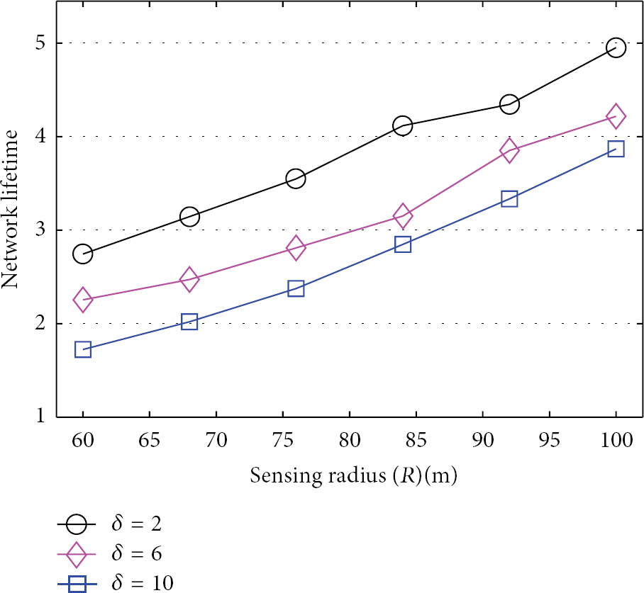
Network lifetime versus R when $L=500$  m, $N=50$ , $M=4$ .

As shown in Figures 8 and 9, the network lifetime is sensitive as the number of nodes and sensing radius. Also the variance has small effect on the lifetime. The lifetime increases as δ decreases. In Figure 8, as the number of nodes increases, the total number of directions in the network increases which can form more barrier sets to prolong the lifetime. In Figure 9, the sensing radius increases, and the total number of directions does not increase. But each direction can overlap more other directions; that is, a barrier set can be formed of a less number of directions. So the number of barrier sets increases in the network which prolongs the network lifetime.

We can observe from Figures 8 and 9 that, generally, increasing the number of sensors (N) or sensing radius (R) can prolong the network lifetime. However, Figure 10 shows a special case of the growth of network lifetime when we increase N or R, respectively. In this simulation, the initial parameters for a given network are $L=500$  m, $N=40$ , $R=40$  m, $M=4$ and, $\delta =2$ .

Figure 10

Network lifetime versus R or N for a given network.

In Figure 10, we can see that when we increase the sensing radius, the network lifetime maintains the momentum of steady growth. The reason is that extending the length of sensing radius for a given network means the target area can be barrier covered by a less number of sensors. The number of barrier sets increases, which leads to the network lifetime increases. However, when we increase the number of sensors, the growth ratio of network lifetime is nonsignificant (like 25 percent and 50 percent). When we deploy more sensors for a given network, the location of each sensor is randomly distributed. The characteristic of randomness may lead to the fact that the number of barrier sets cannot be increased with the sensors we added. So the network lifetime could not be extended under such circumstances.

Figure 11 shows the network lifetime when M varies, $L=500$  m, $R=50$  m, $N=50$ , and $\delta =2$ . We find out that the network lifetime does not monotonically increase or decrease with the number of directions per sensor. On one hand, the number of directions increases meaning more different directions can overlap, which leads to more barrier sets in the network. This results in the increase of the network lifetime. On the other hand, the number of directions increases meaning the sensing region is smaller than before. The total number of directions each direction can overlap becomes less. More sensors are needed to form barriers, leading to the decrease of the network lifetime.

Figure 11

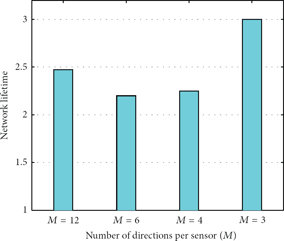
Network lifetime versus M, when $L=500$  m, $R=50$  m, $N=50$ , $\delta =2$ .

We can observe from the results above that each data of simulation results is more than 1, which means our proposed algorithms could prolong the network lifetime. Moreover, network lifetime has proportional relationship to the number of sensors and sensing radius, respectively. The number of directions per sensor also has impact on the network lifetime, but it is not proportional to it.

6. Conclusions and Future Work

Sensor deployment provides important effects in wireless directional sensor networks for barrier coverage. And efficient scheduling algorithm can prolong the network lifetime. In this paper, we have studied the problem of what the probability of barrier coverage depends on, the ESD, and the problem of how to schedule the sensors in the network to prolong the lifetime, the EEBC. We have proposed a deployment model to solve the ESD. An optimization formation was described to solve the EEBC. In the future works, we will consider efficient scheduling for other coverage issues, such as area coverage and target coverage.