Redundancy Model and Boundary Effects Based Coverage-Enhancing Algorithm for 3D Underwater Sensor Networks

Abstract

In the study of three-dimensional underwater sensor networks, the nodes would produce changes in perception range under the influence of environmental factors and their own hardware. Requesting all nodes completely isomorphic is unrealistic. Ignoring boundary effects usually causes the coverage effect of the actual deployment of networks to not reach the anticipated result. This paper firstly presents an underwater sensing model with normal distributed node sensing radius. Secondly, it gives the relationship between expected deployment quality and the number of nodes in the premise of considering boundary effects. Then, it deduces nodes’ redundancy formula based on the sensing model with normal distributed node sensing radius, making node could determine whether itself is a redundant node only based on the number of its neighbour nodes. Furthermore, this paper proposes a redundancy model and boundary effects based coverage-enhancing algorithm for three-dimensional underwater sensor networks (RBCT). Simulation results show that RBCT, compared to similar algorithms, has certain advantages in saving energy and enhancing coverage rate.

1. Introduction

Underwater wireless sensor network (UWSN) has drawn great attention over the recent years for its extensive application prospect in oceanographic hydrological data collection, marine pollution monitoring, marine disaster early-warning, and underwater military reconnaissance [1–8]. Before the emergence of wireless sensor networks (WSNs), underwater data perception and collection depend on costly wired network, while UWSN highly reduces the cost of these underwater applications. UWSN consists of nodes that are cooperatively monitoring in three-dimensional space. According to the three-dimensional UWSN model in [9] proposed by Tezcan et al., the architecture of UWSN consists of anchor, underwater sensor node, and buoy node. Figure 1 depicts the architecture of UWSN. Sensor devices are broadcasted to target area from aircraft or boat. As soon as it comes into contact with water, devices anchor is fixed on the location to avoid floating away with ocean current and deviating from monitoring area which occurred in the model proposed by Tezcan et al. At initial phase, sensor node and the buoy node float on the sea surface. In working phase, according to control algorithm, devices can adjust the length of cable between buoy node and underwater sensor node to deploy the underwater sensor to appointed depth. In the model proposed by Akyildiz et al. [10] and Heidemann et al. [11], underwater sensors anchor in the bottom of sea and communicate via acoustic link. However, in current technical conditions, un derwater acoustic link with narrow band width and high latency can easily be interfered by path loss, noise, multipath effect, and so forth [12, 13]. Therefore, we choose cable as communication medium between underwater sensor nodes and buoy nodes while nodes communicate with each other via wireless communication between buoy nodes. The wireless communication module of buoy nodes has multiple power levels to maintain different communication radius. Buoy can also equip locating device like GPS receiver and energy supply device like solar panel. When buoy receives data from underwater sensor node, it transmits them to base station on the sea or shore and then the data is forwarded to communication satellite, ground network, and terminal user.

Figure 1

Architecture of UWSN.

In WSN, coverage rate is an important indicator to network service quality which is the same in UWSN. Optimizing underwater sensor network coverage has important significance for rationally allocating network space resources, better achieving environmental perception and information acquisition task, and improving the network viability. Terrestrial wireless sensor networks have been studied extensively. In [14], Bai et al. propose and design a series of connected coverage models in three-dimensional wireless sensor networks with low connectivity and full coverage. In [15], Alam and Haas study truncated octahedron deployment strategy to monitor network coverage situation. However, there are little researches on three-dimensional underwater sensor networks. In [16], Alam and Haas point that an underwater sensor network can have significant height which makes it a three-dimensional network unlike a terrestrial network. There are many important sensor network design problems where the physical dimensionality of the network plays a significant role. One such problem is determining how to deploy minimum number of sensor nodes so that all points inside the network are within the sensing range of at least one sensor and all sensor nodes can communicate with each other, possibly over a multihop path. The solution to this problem depends on the ratio of the communication range and the sensing range of each sensor. Under sphere-based communication and sensing model, placing a node at the centre of each virtual cell created by truncated octahedron-based tessellation solves this problem when this ratio is greater than 1.7889. However, for smaller values of this ratio, the solution depends on how much communication redundancy the network needs. Alam and Haas provide solutions for both limited and full communication redundancy requirements. In [17], Akkaya and Newell propose a distributed node deployment scheme which can increase the initial network coverage in an iterative basis. Assuming that the nodes are initially deployed at the bottom of the water and can only move in vertical direction in 3D space, the idea is to relocate the nodes at different depths in order to reduce the sensing overlaps among the neighbouring nodes. The nodes continue to adjust their depths until there is no room for improving their coverage.

In consideration of energy limitation of nodes and the requirement of durability without energy supply, we make use of the redundancy of nodes and heuristic algorithm to make nodes switch to certain state in order to shut down nodes in turn with guaranteed service quality. As a result, node energy is conserved and network lifetime is prolonged. Most of the existing researches are based on the assumption that sensing radius of all nodes is the same while in practice radius varies due to nodes’ characteristics and environmental influence. This paper presents an underwater sensing model with normal distributed node sensing radius and analyzes the redundancy model of these nodes. Furthermore, this paper proposes RBCT algorithm combined with the virtual potential field algorithm to optimize the coverage of networks.

2. Network Model and Problem Description

2.1. Problem Formulation

The coverage enhancement problem of three-dimensional sensor networks can be described as follows. Given a three-dimensional target area, we should create a reasonable mathematical model to find out the relationship between expected deployment quality and the number of nodes in the premise of considering boundary effects. This mathematical model can be used to guide the deployment of nodes. After deployment of certain scale sensor nodes, the problem is how to adjust the nodes’ working conditions to maximize network survival time. When a certain number of nodes are working, the problem is how to adjust the depth of underwater sensor nodes by using coverage optimization algorithms to maximize coverage rate.

We assume that the underwater sensor network has the following properties.

• (1)

The distribution of underwater sensor nodes obeys Boolean sensing model. Underwater sensor node $S_i$ with sensing radius r is located in three-dimensional space Ω. When the distance between the target and $S_i$ is longer than r, the probability of target being detected by $S_i$ is 0; otherwise the probability is 1. Then the sensing area of $S_i$ is a sphere with center $S_i$ and radius r. This sphere is denoted as SD _i , which is composed of all points that satisfies (1). x represents point in the space. $D_{ix}$ represents the distance between point x and $S_i$ . Consider

$$\begin{array}{cc}& S{D}_i=\left\{x\hspace{0.17em}|\hspace{0.17em}x\in \Omega ,D_{ix}⩽r\right\}.\end{array}$$

(1)

(2)

Sensing radius of underwater sensor nodes is normally distributed as $N(r_0,{\delta }^2)$ . $r_0$ is mean value of node sensing radius, also called rated sensing radius.   $\delta$   is standard deviation and $r_0\ge 3.3\delta$ to ensure sensing radius intensively distributed in $[0,2r_0]$ .

(3)

Length of the cable between underwater sensor node and buoy node is adjustable; namely, underwater sensor nodes can accurately move to appointed target location in vertical coordinate axis.

(4)

Each underwater sensor node only needs to know the relative position between itself and its neighbouring nodes, without the need to know the precise location by positioning devices.

In the ideal network model, all the underwater sensor nodes have the same rated sensing radius $r_0$ . But when they are deployed in practical environment, sensing radii of nodes may be influenced by their own characteristics or environmental factor and cause difference. Therefore, we assume that sensing radii of underwater sensor nodes are normally distributed as $r~N(r_0,{\delta }^2)$ . And parameter $r_0$ and δ are restricted to satisfy $r_0\ge 3.3\delta$ . So the probability of sensing radius within $(-\infty ,0)$ will be less than 0.0005. Due to symmetry of normal distribution, the probability of sensing radius within $[0,2r_0]$ will be larger than 0.9990. We can draw a conclusion that sensing radius of underwater nodes within $[0,2r_0]$ is a certain event.

2.2. Related Definition

Definition 1.

Neighbor nodes set ${\psi }_i$ : in WSNs, a pair of nodes is called neighbouring nodes in condition that their Euclidean distance $D_{ij}$ is shorter than twice the sensing radius r

$$\begin{array}{cc}& {\psi }_i=\left\{n_j\hspace{0.17em}|\hspace{0.17em}{D}_{ij}<\mathrm{2}{r}_s,i\ne j\right\}.\end{array}$$

(2)

Definition 2.

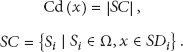
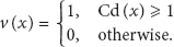
Coverage degree Cd(x): the number of nodes that covered point x is called the coverage degree of point x, denoted as Cd(x):

$$\begin{array}{cc}& \text{Cd}\left(x\right)=\left|SC\right|,\\ SC=\left\{S_i\hspace{0.17em}|\hspace{0.17em}{S}_i\in \Omega ,x\in S{D}_i\right\}.\end{array}$$

(3)

Definition 3.

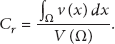
Coverage rate $C_r$ : the coverage rate of WSNs that are deployed in target area Ω is denoted as $C_r$ , defined as follows:

$$\begin{array}{cc}& C_r=\frac{{\int }_{\Omega }v\left(x\right)dx}{V\left(\Omega \right)}.\end{array}$$

(4)

$V(\Omega )$ is the volume of Ω and to any point x satisfies $x\in \Omega$ , and

$$\begin{array}{cc}& v\left(x\right)=\{\begin{array}{cc}\mathrm{1},\hfill & \text{Cd}\left(x\right)⩾\mathrm{1}\hfill \\ \mathrm{0},\hfill & \text{otherwise}.\hfill \end{array}\end{array}$$

(5)

3. Analysis on Coverage Quality and Nodes Deployment Density

Since the boundary effects will have a greater impact on nodes deployment, in this section, we will analyze the relationship between the number of nodes deployed randomly and the initial network coverage expectations under the premise of considering boundary effects.

To a random given node $S_i$ , the distance between $S_i$ and its nearest boundary of monitored region is defined as $d_i$ . The overlap area of a node's sensing area and monitored region is defined as $Ef(d_i)$ , which is also known as effective sensing area of node i. Therefore, if node $S_i$ satisfies $d_i\ge r$ , effective sensing area satisfies Ef $(d_i)=4\pi r_i^3/3$ . If node $S_i$ satisfies $0\le d_i<r_i$ , effective sensing area satisfies $Ef(d_i)<4\pi r_i^3/3$ . Therefore, to a given $r_0>0$ and monitored region Ω, Ω is divided into four areas as shown in Figure 2, namely, Ω(0), Ω(1), Ω(2), and Ω(3). Equation (6) shows the volume of these four areas:

$$\begin{array}{l}\parallel \Omega \left(\mathrm{0}\right)\parallel =\left(l-\mathrm{2}{r}_{\mathrm{0}}\right)\left(m-\mathrm{2}{r}_{\mathrm{0}}\right)\left(n-\mathrm{2}{r}_{\mathrm{0}}\right),\\ \parallel \Omega \left(\mathrm{1}\right)\parallel =\mathrm{4}\left(l-\mathrm{2}{r}_{\mathrm{0}}\right)r_{\mathrm{0}}^{\mathrm{2}}+\mathrm{4}\left(m-\mathrm{2}{r}_{\mathrm{0}}\right)r_{\mathrm{0}}^{\mathrm{2}}+\mathrm{4}\left(n-\mathrm{2}{r}_{\mathrm{0}}\right)r_{\mathrm{0}}^{\mathrm{2}},\\ \parallel \Omega \left(\mathrm{2}\right)\parallel =\mathrm{8}{r}_{\mathrm{0}}^{\mathrm{3}},\\ \parallel \Omega \left(\mathrm{3}\right)\parallel =\mathrm{2}{r}_{\mathrm{0}}\left(l-\mathrm{2}{r}_{\mathrm{0}}\right)\left(m-\mathrm{2}{r}_{\mathrm{0}}\right)+\mathrm{2}{r}_{\mathrm{0}}\left(l-\mathrm{2}{r}_{\mathrm{0}}\right)\left(n-\mathrm{2}{r}_{\mathrm{0}}\right)\\ \hspace{1em}+\mathrm{2}{r}_{\mathrm{0}}\left(n-\mathrm{2}{r}_{\mathrm{0}}\right)\left(m-\mathrm{2}{r}_{\mathrm{0}}\right).\end{array}$$

(6)

Figure 2

Monitored region and related subregion.

Variable M represents the volume that is not covered by nodes in monitored region Ω:

$$\begin{array}{cc}& M={{\displaystyle \int }}_{\Omega }\chi \left(x\right)dx,\\ \chi \left(x\right)=\{\begin{array}{cc}\mathrm{1},\hfill & \text{Cd}\left(x\right)=\mathrm{0}\hfill \\ \mathrm{0},\hfill & \text{Cd}\left(x\right)\ge \mathrm{1}.\hfill \end{array}\end{array}$$

(7)

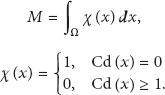
Using Fubini's theorem we obtain that

$$\begin{array}{cc}& E\left(M\right)={{\displaystyle \int }}_{\Omega }E\left(\chi \left(x\right)\right)dx.\end{array}$$

(8)

To a given random point $x\in \Omega$ , $V(x)$ represents the sphere centered at x and with radius $r_0$ . If point x is covered, at least one underwater sensor node is in $V(x)$ ; so we obtain (9). Pr represents the probability of the event occurring. Consider

$$\begin{array}{cc}& E\left\{\chi \left(x\right)\right\}=\text{Pr}\left\{x\mathrm{\hspace{0.17em}\hspace{0.17em}}\text{is}\mathrm{\hspace{0.17em}\hspace{0.17em}}\text{not}\mathrm{\hspace{0.17em}\hspace{0.17em}}\text{covered}\right\}.\end{array}$$

(9)

To a given random point $x\in \Omega$ and underwater sensor node $S_i$ , the probability of x being covered by $S_i$ is defined as $p_{xi}$ . So the probability of x not being covered by $S_i$ is defined as $\overline{p_{xi}}$ . Shown in Figure 2, the location of $S_i$ to monitored region Ω has four possible results: (1) $S_i$ is located in Ω(0); (2) $S_i$ is located in Ω(1); (3) $S_i$ is located in Ω(2); (4) $S_i$ is located in Ω(3). The above four events are mutually exclusive events. Therefore, the probability $\overline{p_{xi}}$ of a random point $x\in \Omega$ not being covered by node $S_i$ can be expressed as (10). $E_V[0]$ , $E_V[1]$ , $E_V[2]$ , and $E_V[3]$ represent the average volume of   $Ef(d_i$ ) when $S_i$ is located in Ω(0), Ω(1), Ω(2), and Ω(3). Consider

$$\begin{array}{l}\overline{p_{xi}}=\mathrm{1}-p_{xi}=\mathrm{1}-({{\displaystyle \int }}_{\Omega \left(\mathrm{0}\right)}\frac{E_V\left[\mathrm{0}\right]}{\parallel \Omega \parallel }dx+{{\displaystyle \int }}_{\Omega \left(\mathrm{1}\right)}\frac{E_V\left[\mathrm{1}\right]}{\parallel \Omega \parallel }dx\\ \phantom{sssssssssssssssssssss}+{{\displaystyle \int }}_{\Omega \left(\mathrm{2}\right)}\frac{E_V\left[\mathrm{2}\right]}{\parallel \Omega \parallel }dx+{{\displaystyle \int }}_{\Omega \left(\mathrm{3}\right)}\frac{E_V\left[\mathrm{3}\right]}{\parallel \Omega \parallel }dx).\end{array}$$

(10)

When $S_i$ is located in Ω(0), the whole sensing area of $S_i$ is contained in monitored region Ω. Consider

$$\begin{array}{cc}& E_V\left[\mathrm{0}\right]=\frac{\mathrm{4}\pi r_{\mathrm{0}}^{\mathrm{3}}}{\mathrm{3}}.\end{array}$$

(11)

When $S_i$ is located in Ω(1), there are two possible situations as shown in Figure 3. Figure 3 shows a cross-sectional view of node's sensing area and monitored region. Parameters a and b represent the distance between node and the two borders of monitored region in Ω(1). $E_V[1]$ can be expressed as in (12). $E_{V1}[1]$ and $E_{V2}[1]$ represent the average volume of   $Ef(d_i)$   in situations 1 and 2.

Figure 3

Two situations of $S_i$ within Ω(1).

Situation 1. The distance between node and the corner of Ω(1) is shorter than $r_0$ .

Situation 2. The distance between node and the corner of Ω(1) is longer than $r_0$ . Consider

$$\begin{array}{l}{E}_V\left[\mathrm{1}\right]=\frac{\left(\mathrm{1}/\mathrm{3}\right)\pi r_0^3}{r_0^3}{E}_{V\mathrm{1}}\left[\mathrm{1}\right]+\left(\mathrm{1}-\frac{\left(\mathrm{1}/\mathrm{3}\right)\pi r_0^3}{r_0^3}\right)E_{V\mathrm{2}}\left[\mathrm{1}\right]\\ =\frac{\pi }{\mathrm{3}}{E}_{V\mathrm{1}}\left[\mathrm{1}\right]+\frac{\mathrm{3}-\pi }{\mathrm{3}}{E}_{V\mathrm{2}}\left[\mathrm{1}\right].\end{array}$$

(12)

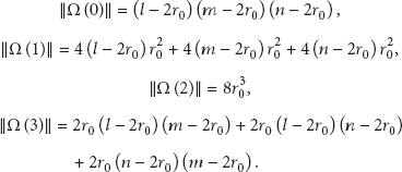
We denote $V_{{\Omega }_{\mathrm{1}}(\mathrm{1})}(a,b)$ and $V_{{\Omega }_{\mathrm{2}}(\mathrm{1})}(a,b)$ as overlap volume of node sensing area and monitored region in situations 1 and 2, respectively. Consider

$$\begin{array}{l}{V}_{{\Omega }_{\mathrm{1}}\left(\mathrm{1}\right)}\left(a,b\right)\\ =\frac{\mathrm{4}\pi r_{\mathrm{0}}^{\mathrm{3}}}{\mathrm{3}}-\frac{\pi {\left(r_{\mathrm{0}}-a\right)}^{\mathrm{2}}\left(a+\mathrm{2}{r}_{\mathrm{0}}\right)}{\mathrm{3}}\\ \hspace{1em}-{{\displaystyle \int }}_0^{a+\sqrt{r_0^2-b^{\mathrm{2}}}}\{\text{arccos}\left[\frac{b}{\sqrt{r_0^2-{\left(a-x\right)}^{\mathrm{2}}}}\right]\left[r_0^2-{\left(a-x\right)}^{\mathrm{2}}\right]\\ \phantom{\text{sssssssssssssssssss}}-b\sqrt{r_0^2-b^{\mathrm{2}}-{\left(a-x\right)}^{\mathrm{2}}}\phantom{\left[\frac{b}{\sqrt{r_0^2-{\left(a-x\right)}^{\mathrm{2}}}}\right]}\}dx,\\ V_{{\Omega }_{\mathrm{2}}\left(\mathrm{1}\right)}\left(a,b\right)=\pi {\left(r_{\mathrm{0}}-x\right)}^{\mathrm{2}}\left(\frac{\mathrm{2}{r}_{\mathrm{0}}+x}{\mathrm{3}}\right)\\ \hspace{1em}+\pi {\left(r_{\mathrm{0}}-y\right)}^{\mathrm{2}}\left(\frac{\mathrm{2}{r}_{\mathrm{0}}+y}{\mathrm{3}}\right),\\ E_{V\mathrm{1}}\left[\mathrm{1}\right]=\frac{\mathrm{4}}{\pi r_{\mathrm{0}}^{\mathrm{2}}}{{\displaystyle \int }}_{\mathrm{0}}^{r_{\mathrm{0}}}{{\displaystyle \int }}_{\mathrm{0}}^{\sqrt{{r_{\mathrm{0}}}^{\mathrm{2}}-a^{\mathrm{2}}}}{V}_{{\Omega }_{\mathrm{1}}\left(\mathrm{1}\right)}\left(a,b\right)dadb=\frac{\pi r_0^3}{\mathrm{4}-\pi },\\ E_{V\mathrm{2}}\left[\mathrm{1}\right]=\frac{\mathrm{92}\pi r_{\mathrm{0}}^{\mathrm{3}}}{\mathrm{4}-\pi }.\end{array}$$

(13)

$E_V[1]$ can be expressed as

$$\begin{array}{cc}& E_V\left[\mathrm{1}\right]=\frac{{\pi }^{\mathrm{2}}{r}_0^3}{\mathrm{9}}+\frac{\pi r_0^3}{\mathrm{18}}.\end{array}$$

(14)

Since Ω(2) is only a small part of Ω, the probability that a node is located in Ω(2) is very small. Even if a node is located in Ω(2), the volume of Ω(2) which is not covered by node is very small compared to Ω. So its impact on the calculation results can be ignored. To simplify the calculations, we set $E_V[2]=r_0^3$ when $S_i$ is located in Ω(2).

Parameter a represents the distance between node $S_i$ within region Ω(3) and the closest border of monitored region Ω. The overlap region of node sensing area and monitored region is shown in Figure 4. $V_{\Omega (\mathrm{3})}(a)$ represents the overlap region of node sensing area and Ω(3). Consider

$$\begin{array}{l}{V}_{\Omega \left(\mathrm{3}\right)}\left(a\right)=\frac{\mathrm{4}\pi r_0^3}{\mathrm{3}}-\pi {\left(r_{\mathrm{0}}-a\right)}^{\mathrm{2}}\left(\frac{\mathrm{2}{r}_{\mathrm{0}}-a}{\mathrm{3}}\right)\\ E_V\left[\mathrm{3}\right]=\frac{\mathrm{1}}{r_{\mathrm{0}}}{{\displaystyle \int }}_{\mathrm{0}}^{r_{\mathrm{0}}}{V}_{\Omega \left(\mathrm{3}\right)}\left(a\right)da\\ =\frac{\mathrm{4}\pi r_0^3}{\mathrm{3}}-\frac{\mathrm{1}}{r_{\mathrm{0}}}{{\displaystyle \int }}_{\mathrm{0}}^{r_{\mathrm{0}}}\pi {\left(r_{\mathrm{0}}-a\right)}^{\mathrm{2}}\left(\frac{\mathrm{2}{r}_{\mathrm{0}}-a}{\mathrm{3}}\right)da\\ =\frac{\mathrm{13}\pi r_0^3}{\mathrm{12}}.\end{array}$$

(15)

Figure 4

Node $S_i$ in Ω(3).

With $E_V[0]$ , $E_V[1]$ , $E_V[2]$ , and $E_V[3]$ , $\overline{p_{xi}}$ can be expressed as (16). To a given random underwater sensor node $S_i$ , we can obtain the expected volume of the overlap region of node sensing area and monitored region as shown in (17):

$$\begin{array}{l}\overline{p_{xi}}=\mathrm{1}-(\parallel \Omega \left(\mathrm{0}\right)\parallel \frac{\mathrm{4}\pi r_{\mathrm{0}}^{\mathrm{3}}}{\mathrm{3}}\\ \phantom{\text{ssssssssssss}}+\parallel \Omega \left(\mathrm{1}\right)\parallel \left(\frac{{\pi }^{\mathrm{2}}{r}_{\mathrm{0}}^{\mathrm{3}}}{\mathrm{9}}+\frac{\pi r_{\mathrm{0}}^{\mathrm{3}}}{\mathrm{18}}\right)\\ \phantom{\phantom{\text{ssssssssss}}\text{ss}}+\parallel \Omega \left(\mathrm{2}\right)\parallel r_{\mathrm{0}}^{\mathrm{3}}+\parallel \Omega \left(\mathrm{3}\right)\parallel \frac{\mathrm{13}\pi r_{\mathrm{0}}^{\mathrm{3}}}{\mathrm{12}})\times {\left(lmn\right)}^{-1},\end{array}$$

(16)

$$\begin{array}{l}E\left[S_i\right]\\ \hspace{1em}=(\parallel \Omega \left(\mathrm{0}\right)\parallel E_V\left[\mathrm{0}\right]+\parallel \Omega \left(\mathrm{1}\right)\parallel E_V\left[\mathrm{1}\right]+\parallel \Omega \left(\mathrm{2}\right)\parallel E_V\left[\mathrm{2}\right]\\ \phantom{sssss}+\parallel \Omega \left(\mathrm{3}\right)\parallel E_V\left[\mathrm{3}\right])\times {\left(\parallel \Omega \parallel \right)}^{-1}\\ \hspace{1em}=(\frac{\mathrm{4}}{\mathrm{3}}\pi r^{\mathrm{3}}\left(l-\mathrm{2}r\right)\left(m-\mathrm{2}r\right)\left(n-\mathrm{2}r\right)\\ \hspace{1em}\hspace{1em}\hspace{1em}+\left(\frac{{\pi }^{\mathrm{2}}{r}^{\mathrm{3}}}{\mathrm{9}}+\frac{\pi r^{\mathrm{3}}}{\mathrm{18}}\right)\\ \hspace{1em}\hspace{1em}\hspace{1em}\times \left[\mathrm{4}\left(m-\mathrm{2}r\right)r^{\mathrm{2}}+\mathrm{4}\left(n-\mathrm{2}r\right)r^{\mathrm{2}}+\mathrm{4}\left(l-\mathrm{2}r\right)r^{\mathrm{2}}\right]\phantom{\phantom{\frac{\mathrm{4}}{\mathrm{3}}}})\\ \hspace{1em}\hspace{1em}\times {\left(lmn\right)}^{-1}\\ \hspace{1em}\hspace{1em}+(\mathrm{8}{r}^{\mathrm{6}}+\frac{\mathrm{13}}{\mathrm{6}}\pi r^{\mathrm{4}}[\left(m-\mathrm{2}r\right)\left(l-\mathrm{2}r\right)\\ \phantom{\text{sssssssssssssssssssssssss}}+\left(n-\mathrm{2}r\right)\left(l-\mathrm{2}r\right)\\ \phantom{\text{sssssssssssssssssssssssss}}+\left(m-\mathrm{2}r\right)\left(n-\mathrm{2}r\right)]\phantom{\frac{\mathrm{13}}{\mathrm{6}}})\\ {\hspace{1em}\hspace{1em}\times \left(lmn\right)}^{-1}.\end{array}$$

(17)

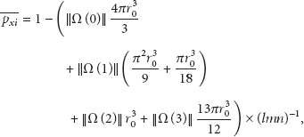
When the number of nodes deployed in Ω is N, we obtain

$$\begin{array}{l}E\left\{\chi \left(x\right)\right\}={\displaystyle \prod }_{i=\mathrm{1}}^N\overline{p_{xi}}={\left(\overline{p_{xi}}\right)}^N,\\ E\left(M\right)\\ \hspace{1em}={{\displaystyle \int }}_{\Omega }{\left(\overline{p_{xi}}\right)}^{N}dx\\ \hspace{1em}={{\displaystyle \int }}_{\Omega }(\mathrm{1}-(\parallel \Omega \left(\mathrm{0}\right)\parallel \frac{\mathrm{4}\pi r_0^3}{\mathrm{3}}+\parallel \Omega \left(\mathrm{1}\right)\parallel \\ \phantom{ssssssssssssssss}\times \left(\frac{{\pi }^{\mathrm{2}}{r}_0^3}{\mathrm{9}}+\frac{\pi r_0^3}{\mathrm{18}}\right)+\parallel \Omega \left(\mathrm{2}\right)\parallel r_0^3\\ {\phantom{ssssssssssssssss}+\parallel \Omega \left(\mathrm{3}\right)\parallel \frac{\mathrm{13}\pi r_0^3}{\mathrm{12}})\times {\left(lmn\right)}^{-1})}^{N}dx\\ \hspace{1em}=\parallel \Omega \parallel (\mathrm{1}-(\parallel \Omega \left(\mathrm{0}\right)\parallel \frac{\mathrm{4}\pi r_0^3}{\mathrm{3}}\\ \phantom{sssssssssssss}\hspace{1em}\hspace{1em}+\parallel \Omega \left(\mathrm{1}\right)\parallel \left(\frac{{\pi }^{\mathrm{2}}{r}_0^3}{\mathrm{9}}+\frac{\pi r_0^3}{\mathrm{18}}\right)+\parallel \Omega \left(\mathrm{2}\right)\parallel r_0^3\\ {\phantom{ssssssssssssssss}\hspace{1em}\hspace{1em}+\parallel \Omega \left(\mathrm{3}\right)\parallel \frac{\mathrm{13}\pi r_0^3}{\mathrm{12}})\times {\left(lmn\right)}^{-1})}^N.\end{array}$$

(18)

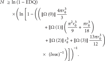
When N nodes are deployed in Ω, we use EDQ (expected deployment quality) to represent the expected deployment quality of the three-dimensional underwater sensor networks. Therefore, if EDQ is required to achieve a certain value in considering boundary effect, the number of nodes deployed in Ω should satisfy (20):

$$\begin{array}{l}\text{EDQ}=\mathrm{1}-\frac{E\left(M\right)}{\parallel \Omega \parallel }\\ =\mathrm{1}-(1-(\parallel \Omega \left(\mathrm{0}\right)\parallel \frac{\mathrm{4}\pi r_0^3}{\mathrm{3}}\\ \phantom{ssssssssssss}\hspace{1em}+\parallel \Omega \left(\mathrm{1}\right)\parallel \left(\frac{{\pi }^{\mathrm{2}}{r}_0^3}{\mathrm{9}}+\frac{\pi r_0^3}{\mathrm{18}}\right)\\ \phantom{ssssssssssss}\hspace{1em}+\parallel \Omega \left(\mathrm{2}\right)\parallel r_0^3+\parallel \Omega \left(\mathrm{3}\right)\parallel \frac{\mathrm{13}\pi r_0^3}{\mathrm{12}})\\ \phantom{sssssssss}{\times {\left(lmn\right)}^{-1}\phantom{\parallel \Omega \left(\mathrm{0}\right)\parallel \frac{\mathrm{4}\pi r_0^3}{\mathrm{3}}})}^N,\end{array}$$

(19)

$$\begin{array}{l}N\hspace{0.17em}\ge \hspace{0.17em}ln\left(1-\text{EDQ}\right)\hfill \\ \hspace{1em}\hspace{1em}\times (ln[1-((\Vert \Omega \left(0\right)\Vert \frac{4\pi r_0^3}{3}\hfill \\ \hspace{1em}\hspace{1em}\hspace{1em}\hspace{1em}\hspace{1em}\hspace{1em}\hspace{1em}+\Vert \Omega \left(1\right)\Vert \left(\frac{{\pi }^2{r}_0^3}{9}+\frac{\pi r_0^3}{18}\right)\hfill \\ \hspace{1em}\hspace{1em}\hspace{1em}\hspace{1em}\hspace{1em}\hspace{1em}\hspace{1em}+\Vert \Omega \left(2\right)\Vert r_0^3+\Vert \Omega \left(3\right)\Vert \frac{13\pi r_0^3}{12})\hfill \\ \hspace{1em}\hspace{1em}\hspace{1em}\hspace{1em}\hspace{1em}\hspace{1em}\hspace{0.17em}\hspace{0.17em}{\times \hspace{0.17em}{\left(lmn\right)}^{-1})])}^{-1}.\hfill \end{array}$$

(20)

4. Redundancy Model Based Coverage-Enhancing Algorithm for 3D Underwater Sensor Networks

With the relationship of the number of underwater sensor nodes N and EDQ, we can deploy randomly a number of nodes more than the required number according to (19) and (20). The certain strategy can be used to adjust the working states and positions of some nodes in order to increase the lifetime and coverage rate of network. In this section, we propose a strategy based on redundancy of node. Each node firstly decides their working states according to redundancy. Then the working nodes use the virtual force algorithm to adjust their positions in the vertical direction.

4.1. Analysis on Node Redundancy

Definition 4.

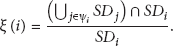
Node redundancy ξ (i): to a random underwater sensor node $S_i$ , there is an overlap region of its sensing area and the sensing area of all its neighbouring nodes. The proportion of the overlap area to the sensing area of itself is called the redundancy of the node $S_i$ . $\xi (i)$ can be expressed as

$$\begin{array}{cc}& \xi \left(i\right)=\frac{\left({{\displaystyle \bigcup }}_{j\in {\psi }_i}S{D}_j\right)\cap S{D}_i}{S{D}_i}.\end{array}$$

(21)

To adjust the working states of nodes based on its redundancy, two problems should be solved. One is the criterion for determining whether a node is redundant, the other is how to schedule redundant node. This section is focused on the first problem and the other one will be discussed in the next section. One way to calculate the redundancy of node is using positioning devices to obtain location information. However, this approach is a huge burden for cost and energy consumption of networks. We build a probabilistic model. Node can calculate its redundancy based on the number of its neighbouring nodes using this probabilistic model. Then each node can determine whether it is a redundant node.

All nodes are randomly and uniformly deployed in monitored region Ω, so each node locates in a random point in Ω with probability   $1/\parallel \Omega \parallel$ . Given two underwater sensor nodes $S_a$ and $S_b$ , their maximum sensing radii are, respectively, marked as $r_a$ and $r_b$ . If there is overlap region in sensing area of   $S_a$   and   $S_b$ ,   $S_b$   needs to be located in the sphere where the center is   $S_a$   and the radii is   $r_a+r_b$ . If there is at least one point x in the sensing areas of   $S_a$   and   $S_b$   simulaneously, $S_b$ needs to be located in the sphere where the center is x and the radii is   $r_b$ . If there is at least one point x in the sensing areas of $S_a$ and $S_b$ simultaneously, $S_b$ needs to be located in the sphere where centered x with radius $r_b$ . Therefore, the probability of that there is at least one point in the sensing areas of $S_a$ and $S_b$ simultaneously can be expressed as

$$\begin{array}{cc}& p_{ab}=\frac{\left(\mathrm{4}/\mathrm{3}\right)\pi r_b^{\mathrm{3}}\times \mathrm{1}/\parallel \Omega \parallel }{\left(\mathrm{4}/\mathrm{3}\right)\pi {\left(r_a+r_b\right)}^{\mathrm{3}}\times \mathrm{1}/\parallel \Omega \parallel }=\frac{r_b^{\mathrm{3}}}{{\left(r_a+r_b\right)}^{\mathrm{3}}}.\end{array}$$

(22)

Sensing radii of $S_a$ and $S_b$ are normally distributed as   $N(r_0,{\delta }^2)$   and $r_0\ge 3.3\delta$ , so the expected value of $p_{ab}$ can be expressed as

$$\begin{array}{l}E\left(p_{ab}\right)\\ \hspace{1em}=\frac{\mathrm{1}}{\mathrm{2}\pi {\delta }^{\mathrm{2}}}{\iint }_{\mathrm{0}}^{\mathrm{2}{r}_{\mathrm{0}}}\frac{r_b^{\mathrm{3}}}{{\left(r_a+r_b\right)}^{\mathrm{3}}}{e}^{-\left({\left(r_a-r_{\mathrm{0}}\right)}^{\mathrm{2}}+{\left(r_b-r_{\mathrm{0}}\right)}^{\mathrm{2}}\right)/\mathrm{2}{\delta }^{\mathrm{2}}}d{r}_{b}d{r}_b\\ \hspace{1em}=\frac{\mathrm{1}}{\mathrm{4}}-\frac{e^{-r_{\mathrm{0}}}}{\mathrm{4}}.\end{array}$$

(23)

The probability of event that there is overlap region in sensing area of $S_a$ and $S_b$ is denoted as $p_{ab}$ , so the opposite event that there is no overlap region in sensing area of $S_a$ and $S_b$ is denoted as $\overline{p_{ab}}=\mathrm{1}-p_{ab}$ . If node $S_a$ has k neighbouring nodes, then the probability of a random point in sensing area of $S_a$ being covered by at least one of its k neighbouring nodes is denoted as $p_{ak}$ . So the probability of opposite event that any point in sensing area of $S_a$ not being covered by its k neighbouring nodes is denoted as $\overline{p_{ak}}$ . $\overline{p_{ak}}$ can be expressed as (24), so $p_{ak}$ can be expressed as (25)

$$\begin{array}{cc}& \overline{p_{ak}}={\left(\overline{p_{ab}}\right)}^k={\left(\mathrm{1}-p_{ab}\right)}^k,\end{array}$$

(24)

$$\begin{array}{cc}& p_{ak}=\mathrm{1}-\overline{p_{ak}}=\mathrm{1}-{\left(\mathrm{1}-p_{ab}\right)}^k.\end{array}$$

(25)

Definition 5.

Redundant node: node $S_i$ is called redundant node in condition that its expected value of redundancy is greater than EDQ of network. It can be expressed as (26). Because when node $S_i$ satisfies (26), the proportion of overlap region in sensing area of $S_i$ to its neighbour nodes exceeds EDQ. If we let $S_i$ into sleep, the coverage rate of its original sensing area could also achieve EDQ:

$$\begin{array}{cc}& E\left(\xi \left(i\right)\right)\ge \text{EDQ}.\end{array}$$

(26)

Based on the above analysis, we can know that node $S_i$ is redundant node when the number of neighbour nodes of $S_i$ satisfies

$$\begin{array}{cc}& k\ge \frac{\ln \left(\mathrm{1}-\text{EDQ}\right)}{\ln \left(\mathrm{3}/\mathrm{4}+\left(\mathrm{1}/\mathrm{4}\right)e^{-r_{\mathrm{0}}}\right)}.\end{array}$$

(27)

4.2. Node Scheduling Algorithm Based on Virtual Force

We have made a detailed analysis on virtual force of three-dimensional sensor networks in [18]. We will only illustrate some necessary concepts in this section. We point out in [18] that the coverage rate fluctuates significantly and nodes adjust location frequently in late stage of traditional coverage optimization algorithms. For these shortcomings, we improve the algorithm by using coverage impact factor and central computing nodes.

Definition 6.

Coverage impact factor: coverage impact factor ${\mu }_i$ characterizes the impact on network coverage when the location of node $S_i$ is changed. We define it as follows. $C_r$ represents the current coverage rate. $C_r^{\prime }$ represents the coverage rate after changing the location of node $S_i$ . Consider

$$\begin{array}{cc}& {\mu }_i=\{\begin{array}{cc}\mathrm{1},\hfill & C_r^{\prime }>C_r\hfill \\ \mathrm{0},\hfill & C_r^{\prime }\le C_r.\hfill \end{array}\end{array}$$

(28)

We add some central computing nodes into the monitored region. All underwater sensor nodes should be within the communication ranges of central computing nodes. Underwater sensor nodes send their target location information to the nearest central computing node. The central computing nodes calculate the coverage impact factors of the nodes within their communication ranges once every slot time and send them to each underwater sensor node. Then each node decides whether to adjust its location based on the coverage impact factor. The number and positions of central computing nodes are determined according to the actual condition of application.

Node $S_i$ is under action of the repulsion of node $S_j$ which is defined in (29). $S_i$ is located at $S_i$ and $S_j$ is located at $S_i$ .   $k$   represents the repulsion coefficient which is a positive constant. The resultant force of repulsion at $S_i$   is $\overrightarrow{F_i}$ . Consider

$$\begin{array}{cc}& \overrightarrow{F_{ij}}=\{\begin{array}{cc}\frac{k}{{D_{ij}}^{\mathrm{2}}}\left(\frac{S_i-S_i}{D_{ij}}\right),\hfill & D_{ij}<\mathrm{2}r\hfill \\ \mathrm{0},\hfill & D_{ij}\ge \mathrm{2}r,\hfill \end{array}\end{array}$$

(29)

$$\begin{array}{cc}& \overrightarrow{F_i}={\displaystyle \sum }_{S_j\in {\psi }_i}\overrightarrow{F_{ij}}.\end{array}$$

(30)

In UWSN, we can only adjust the length of cable between buoy node and underwater sensor node to change the location of underwater sensor nodes. The underwater sensor nodes can achieve coverage enhancement only by adjusting their location in the vertical direction. $\overrightarrow{F_i}$ and the moving distance of $S_i$ determine the target position of $S_i$ together. ${\text{dis}}_{\max }$ is denoted as the maximum single movement distance while the actual movement distance of the node dis _i satisfies (31). The nodes do not move at a fixed length in order to speed up the optimization. At the same time, we set a minimum single movement distance ${\text{dis}}_{\min }$ . When $\text{di}{\text{s}}_i<{\text{dis}}_{\min }$ , the virtual force suffered by $S_i$ reaches equilibrium and there is no need to adjust the location of $S_i$ any more. When all nodes in monitored region have reached equilibrium, we believe that the network has reached equilibrium and the algorithm would be terminated:

$$\begin{array}{cc}& \text{di}{\text{s}}_i=\frac{\parallel \overrightarrow{F_i}\parallel }{\parallel \overrightarrow{F_i}\parallel +\mathrm{1}}\text{di}{\text{s}}_{\max }.\end{array}$$

(31)

4.3. Algorithm Description

Based on the above analysis, to a given EDQ of 3D underwater sensor networks, we firstly calculate the minimum number of nodes N that need to be deployed according to (20). Then we randomly deploy more than N underwater sensor nodes in monitored region Ω. At this time, buoy nodes are randomly distributed on the surface area, and the length of cable between buoy nodes and underwater sensor nodes is random. After completion of the initial deployment, each node firstly collects the information of its neighbour nodes and determines whether it is a redundant node itself. If it is a redundant node, then the node will be set to sleep mode or does not change its working state. Then we use the virtual force algorithm to adjust the position of working nodes. After a round of adjustment, nodes (including those sleeping nodes) change their working states again according to the number of their neighbour nodes. Particularly, at this time we no longer use original EDQ as a factor to determine whether a node is redundant node in order to rapidly enhance the coverage rate of monitored area. We replace EDQ with coverage rate of monitored area as the judgment criteria. The nodes constantly circulate the above processes. Take node $S_i$ as an example; after completion of the initial deployment, RBCT algorithm is described as in Algorithm 1, where $A_i$ is the computing node nearest to underwater sensor node $S_i$ .

Algorithm 1

Input: information of $S_i$ and its neighbour nodes

Output: working state and final location information of $S_i$

(1) $t\leftarrow 0$ ; //initialization

(2) Set loop maximum $t_{\max }$ ;

(3) while ( $t<t_{\max }$ )

(4)  Update current location information of $S_i$ ;

(5)  Update the neighbour nodes set ${\psi }_i$ and the number k of ${\psi }_i$ ;

(6)  Replay EDQ with current coverage rate of monitored area, and determine whether $S_i$ is a redundant node;

(7)  if ( $S_i$ is a redundant node)

(8)    Set $S_i$ into sleeping mode;

(9)  else

(10)    if ( $S_i$ is sleeping)

(11)      Wake up $S_i$ ;

(12)     $\overrightarrow{F_i}\leftarrow 0$ ;

(13)    for ( $j=0$ ; $j<k$ ; j++)

(14)       Calculate the virtual repulsive force $\overrightarrow{F_{ij}}$ on node Si from $S_j$ ;

(15)        $\overrightarrow{F_i}\leftarrow \overrightarrow{F_i}+\overrightarrow{F_{ij}}$ ;

(16)    Calculate the moving distance $\text{di}{\text{s}}_i$ in the vertical direction and the target position $S_i^{\prime }(x^{\prime },y^{\prime },z^{\prime })$ of $S_i$ ;

(17)    if $((\text{di}{\text{s}}_i>\text{di}{\text{s}}_{\min })\&\&(S_i^{\prime }(x^{\prime },y^{\prime },z^{\prime })\ne S_i(x,y,z)))$

(18)     Send the target position $S_i^{\prime }(x^{\prime },y^{\prime },z^{\prime })$ of Si to its nearest computing node $A_i$ ;

(19)     Wait to receive the coverage impact factor ${\mu }_i$ from $A_i$ ;

(20)     if ( ${\mu }_i=1$ )

(21)        Move $S_i$ to the target position;

(22)     else

(23)        sleep( $\mathrm{\Delta }t$ );

(24)   $t\leftarrow t+\mathrm{1}$ ;

(25) end;

RBCT algorithm is running on   $A_i$   as in Algorithm 2.

Algorithm 2

Input: current location and target location information of all nodes within the communication range of $A_i$ ;

Output: coverage impact factor

(1) Get the initial location information of all nodes within communication range;

(2) Calculate the initial coverage rate $C_r$ of monitored region $\mathrm{\Omega }$ ;

(3) while (1)

(4)  Update $C_r$ ;

(5)  Receive target location information of all nodes within the communication range. We use node $S_i$ as an example;

(6)  Calculate the coverage rate $C_r^{\prime }$ of monitored region $\mathrm{\Omega }$ after $S_i$ moving to target location;

(7)  Calculate the coverage impact factor of $S_i$ ;

(8)  Send the coverage impact factor ${\mu }_i$ to $S_i$ ;

(9)  sleep( $\mathrm{\Delta }t$ );

(10) end;

5. Algorithm Simulations and Performance Analysis

In this section, we firstly analyze the convergence of RBCT algorithm. Secondly, we use a specific case to illustrate the coverage enhancement effect to a three-dimensional sensor network. Finally, we compare RBCT algorithm with other similar algorithms by different values of key parameters. Specific values of parameters are shown in Table 1.

Table 1

Experiment parameters.

Target region	$\mathrm{30000}*\mathrm{30000}*\mathrm{30000}$  m3
Distribution mode	Randomly distributed
Number of underwater sensor nodes N	200–500
Average maximum sensory radius $r_0$	2–3.5 km
Maximum single movement distance $\text{di}{\text{s}}_{\max }$	1–4 km
Factor of virtual repulsive force k	10
Expected deployment quality EDQ	0.4–0.8

5.1. Algorithm Convergence Analysis

We carry out a group of experiments with five kinds of EDQ so as to analyze RBCT algorithm convergence. To a given EDQ, we can calculate the number of nodes that need to be deployed through (20). According to every EDQ, we randomly produce 20 topological structures, respectively, and calculate the algorithm convergence times and average. Experimental data is shown in Table 2 with parameters $r_0=3\hspace{0.17em}\text{km}$ and ${\text{dis}}_{\max }=3\hspace{0.17em}\text{km}$ .

Table 2

Convergence analysis on experimental data.

EDQ	Number of nodes N	Initial coverage rate%	Ultimate coverage rate%	The number of loops
0.4	131	39.4	50.3	23.5
0.5	182	48.7	65.2	22.7
0.6	237	58.5	76.3	25.6
0.7	309	68.9	86.1	25.3
0.8	407	79.2	92.8	26.1

Based on the above analysis we can reach a conclusion that the convergence of RBCT algorithm, that is, the adjustment number of times, does not change conspicuously along with EDQ or N. The value ranges from 22 to 27; thus, RBCT algorithm can improve the coverage of monitored region in a short time and has a nice convergence.

5.2. Case Study

Figure 5 records the coverage curves of monitored region in experiments of algorithm convergence analysis. Figure 5 shows that due to the influence of RBCT algorithm, coverage rate is constantly improving. When the network reaches a steady state, coverage rates remain unchanged and RBCT algorithm ends. The coverage rates do not present a fluctuating state during the execution of RBCT algorithm since the introduction of coverage impact factor. By RBCT algorithm, the coverage rates are raised to 50.3%, 65.2%, 76.3%, 86.1%, and 92.8% without changing the number of initial nodes. We can know through (20) that at least 185, 272, 367, 498, and 661 nodes are separately needed to achieve thus coverage rate by the way of random deployment. It means that we have saved 54, 90, 130, 189, and 254 nodes, respectively. From this set of data we can see that the higher the EDQ, the larger the number of nodes that can be saved by RBCT algorithm. RBCT algorithm greatly reduces the cost and complexity of network.

Figure 5

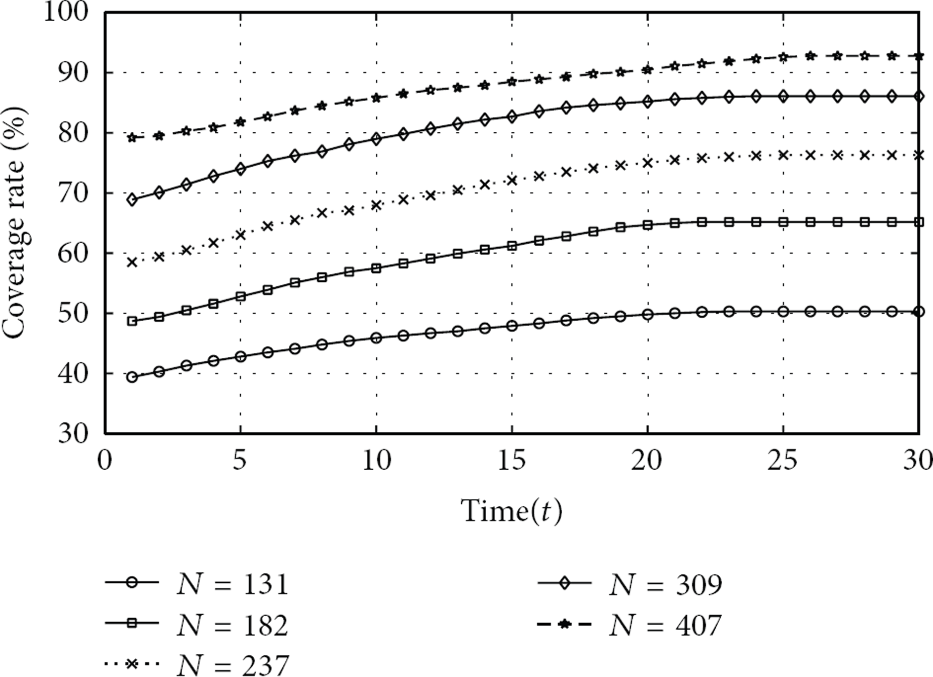
Coverage curves in different scale of nodes.

In order to intuitively view the coverage condition of monitored region, we draw it graphically as shown in Figure 6. We take one random topology as study case when the number of nodes is 407. Figure 6 shows the projection of monitored region in the vertical direction. The initial coverage rate is basically consistent with EDQ and from Figure 6(a) we can see that overlap region and fade zone are significant in network for the randomness of deployment. By means of RBCT algorithm, redundant nodes change into sleeping mode, and then working nodes adjust their locations in the vertical direction. Proportion of fade zone is constantly reducing when RBCT algorithm is running. Finally, we reach the purpose of covering the maximum monitored region with minimal number of nodes, which is shown in Figure 6(c).

Figure 6

Coverage optimization under RBCT algorithm when $N=\mathrm{407}$ .

We carry out a group of experiments as the following to prove that RBCT algorithm can reduce the energy consumption of networks. We assume that the initial energy of each underwater sensor node is 100. If one node is in working state and does not need to adjust the position, then the energy consumption of this node is 1 within one time step. If one node is in sleeping state, then the energy consumption of this node is 0. The energy consumption of every position adjustment is 1. When the energy of a node is reduced to 0, the status of this node is marked as dead. If more than 10% of all nodes are marked as dead, we identify the network is paralyzed. We record the time from initial deployment of the nodes to the paralysis of network as the lifetime of network. We randomly produce 30 topological structures with $\text{EDQ}=0.6$ . 10 of them execute RBCT algorithm and 10 of them execute PCPE algorithm proposed in [19]. We, respectively, record the lifetime of networks and average. Experimental results are shown in Figure 7. As shown in Figure 7, the lifetime of networks without optimization is longer than the other two, since the nodes only consume energy in communications without changing locations. RBCT algorithm reduces the lifetime of networks, but still better than the effect of PCPE algorithm. Coverage optimization algorithms improve the coverage rate of monitored region while reducing the lifetime of networks. The final coverage rates of monitored region are shown in Figure 8. We can see from Figure 8 that RBCT algorithm has the best effect on coverage rate of monitored region. Thus, RBCT algorithm improves the coverage rate with reducing the lifetime of networks for the price.

Figure 7

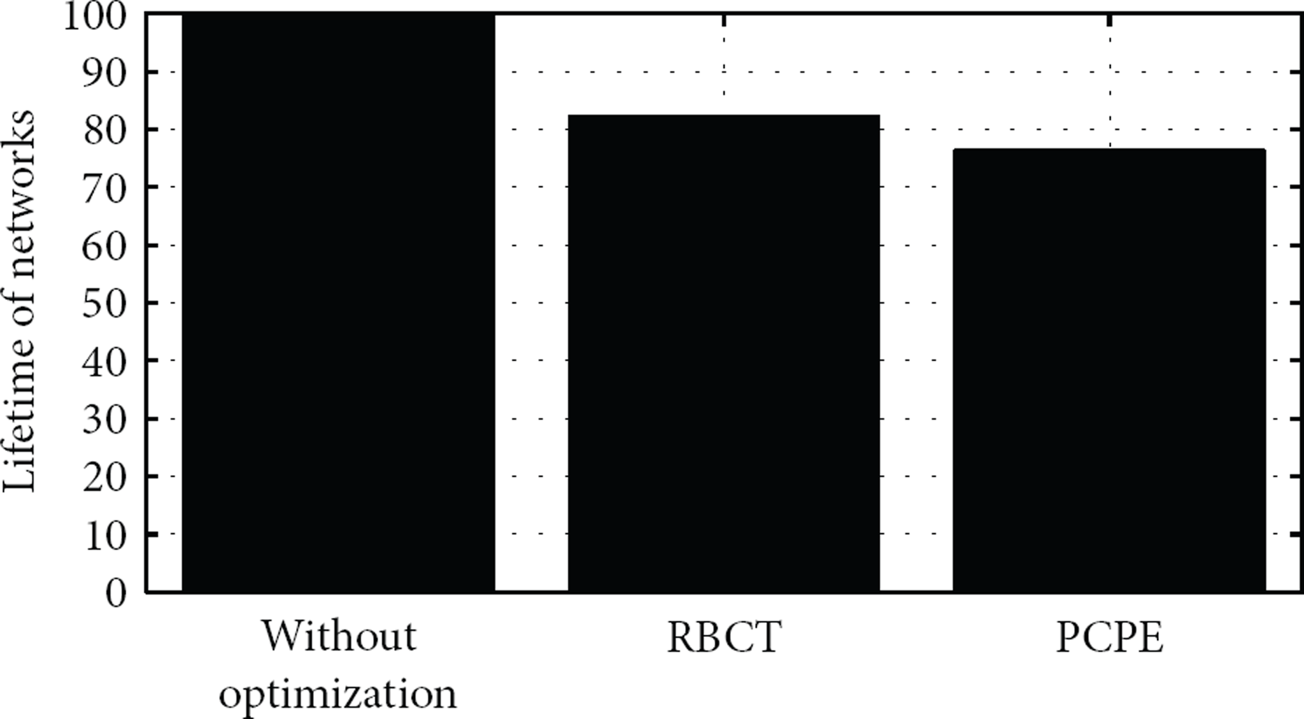
Effect on lifetime with different optimizations.

Figure 8

Effect on coverage rate with different optimizations.

5.3. Comparative Analysis of Algorithms

In this section, a series of simulation experiments are conducted to illustrate the effect on the performance of RBCT algorithm from the three key parameters. They are expected deployment quality of monitored region EDQ, average maximum sensory radius $r_0$ , and maximum single movement distance ${\text{dis}}_{\max }$ . We take PCPE algorithm and PFCEA algorithm proposed in [19, 20] as comparison algorithms. We compare RBCT algorithm to them and analyze their performances. We take a number of simulations for each set of parameters and record experimental data, respectively.

As shown in Figure 9, we conduct the simulation experiments with different EDQ. Other experimental parameters satisfy that $r_0=3\hspace{0.17em}\text{km}$ and ${\text{dis}}_{\max }=3\hspace{0.17em}\text{km}$ . In the simulation experiments of Figure 10, we use $r_0$ as variable parameter and other experimental parameters satisfy that $N=300$ and ${\text{dis}}_{\max }=3\hspace{0.17em}\text{km}$ . We can see from the curves in Figures 9 and 10 that the effect on coverage rate from EDQ is similar to $r_0$ . It is because the greater the value of EDQ is, the larger the number of nodes in the initial deployment is. The shorter the $r_0$ is, the smaller the coverage area of a single node is. When ${\text{dis}}_{\max }$ is fixed, smaller value of EDQ and $r_0$ leads to smaller initial coverage rate. As the EDQ and $r_0$ increase, the value of ΔC _r and initial coverage rate increase together. However, when the value of variable parameters exceeds a certain limitation, the growth trend of ΔC _r and initial coverage rate will slow down. The reason is that the increase of EDQ and $r_0$ leads to a higher initial coverage rate and greatly decreases the probability that several communicational adjacent nodes form coverage fade zone which undoubtedly weakens the performance of RBCT algorithm.

Figure 9

Convergent curves with different EDQ.

Figure 10

Convergent curves with different $r_0$ .

As shown in Figures 11 and 12, we conduct the simulation experiments with different ${\text{dis}}_{\max }$ . Other experimental parameters satisfy that $N=300$ and $r_0=3\hspace{0.17em}\text{km}$ . The experiment result shows that the greater the value of ${\text{dis}}_{\max }$ is, the smaller the value of $\Delta C_r$ is. It should be noted that different ${\text{dis}}_{\max }$ will have a significant impact on the number of loops. As shown in Figure 12, in a certain range the smaller the value of ${\text{dis}}_{\max }$ is, the bigger the number of loops will be. In particular when the value of ${\text{dis}}_{\max }$ is less than 2 km, the algorithm loops increased dramatically, while the increase of network coverage optimization effect is not obvious. Thus, we should select an appropriate ${\text{dis}}_{\max }$ in practical applications to avoid slow convergence rate and a large number of nodes’ energy consumption.

Figure 11

Convergent curves with different ${\text{dis}}_{\max }$ .

Figure 12

Relationship between the number of loops and ${\text{dis}}_{\max }$ .

As can be seen from Figures 9 to 12 compared to PCPE algorithm and PFCEA algorithm, with the same parameter value, the proposed RBCT algorithm increases the coverage quality the most significant after the optimization of the initial deployment, which illustrates the superiority of this algorithm.

6. Conclusion

This paper derives the relationship between the number of nodes and the coverage quality of 3D underwater sensor network using mathematical analysis and proposes RBCT algorithm based on the redundancy model of nodes to improve the coverage of monitored region and prolong the lifetime of network. The coverage impact factor is introduced to reduce profitless movement and further improve coverage optimization. In simulation experiments, we firstly verify the convergence of the algorithm and then the effect on the algorithm from the key parameters and validity of RBCT are demonstrated by the comparisons among RBCT, PCPE, and PFCEA. The proposed algorithm effectively improves the coverage performance of network but many issues in this paper could be improved. We can see from the simulation experiments that the actual initial coverage rate of monitored region is still slightly lower than EDQ. It shows that the theoretical analysis of this paper could be improved which is for further study.