Vehicle State Information Estimation with the Unscented Kalman Filter

Abstract

The vehicle state information plays an important role in the vehicle active safety systems; this paper proposed a new concept to estimate the instantaneous vehicle speed, yaw rate, tire forces, and tire kinemics information in real time. The estimator is based on the 3DoF vehicle model combined with the piecewise linear tire model. The estimator is realized using the unscented Kalman filter (UKF), since it is based on the unscented transfer technique and considers high order terms during the measurement and update stage. The numerical simulations are carried out to further investigate the performance of the estimator under high friction and low friction road conditions in the MATLAB/Simulink combined with the Carsim environment. The simulation results are compared with the numerical results from Carsim software, which indicate that UKF can estimate the vehicle state information accurately and in real time; the proposed estimation will provide the necessary and reliable state information to the vehicle controller in the future.

1. Introduction

Active safety is all about technical solutions that help the drivers avoid accidents or significantly reduce the possibilities of the accidents. These include braking systems, like ABS, traction control systems, and electronic stability control systems that interpret the signals from various sensors to help drivers control the vehicle or give a warning to driver under various road conditions as well as the driving maneuvers. And the performances of the controller rely heavily on the accurate vehicle states information. Some of the required vehicle state information is easy to measure by the sensors which exist in model vehicle, such as the spin speed of four wheels, but others are difficult to detect due to the expense, complexity, and the technological limits. Reducing sensor is a potential approach to cut down the cost and improve the reliability and performance of the controller. State estimation is an algorithm which prides the internal state of a given system in real time; the algorithm uses the online measurements as inputs and obtains the estimated values. It provides the basis of many practical applications and attracts increasing attention in the field of automobile industry, especially in the vehicle active safety research field [1–4].

Accurate and real-time vehicle state information is necessary for the vehicle dynamic controller; there are a lot of researchers who have proposed some approaches to estimate the vehicle state and parameters. Zhao et al. [5] proposed the tire force estimation method by using sliding model observer, and its drawback is that the method calls for the high speed computational hardware because of the complicated and high order vehicle model. Tims [6] investigated the approach to reduce sensors used in active suspension control; he used a relative displacement sensor to estimate vehicle corner sprung mass velocity, but he did not consider the potential for phase advance or lag in the estimation of velocity, especially for the large pitch and roll motion; it may deteriorate the vehicle comfort caused by the signal's time delay. Wenzel et al. [7] used the dual extended Kalman filter to estimate vehicle states and parameters; the advantage is that two Kalman filters can run in parallel; which can also work as a signal EKF estimator by simply “turn off” one of them; however, the method is under the hypothesis that the tire-road friction coefficient is known. In [8], Zong et al. applied the dual extended Kalman filter to estimate the tire-road adhesion coefficient based on full vehicle model; nevertheless, it is difficult to acquire the accurate Jacobi matrix, especially for the high order vehicle model or when the tire forces are working in the saturation zone.

The main contributions of this study are as follows: we proposed a UKF estimator based on a 3DoF vehicle model for state estimation of a class of nonlinear systems; this estimation algorithm is to estimate the longitudinal and lateral velocity and the tire characteristics. And considering the limitations of the linear tire model and the complication of the Magic Formula tire model, the paper proposed a piece-wise linear tire model. The paper is organized as follows: firstly, piece-wise linear tire model and the vehicle model are introduced in Sections 2 and 3, respectively. In Section 4, the unscented Kalman filter is introduced in detail. In Section 5 the estimation results of the KF with the linear bicycle model, UKF with linear bicycle model, and Carsim outputs are presented as the comparison. At last, the discussion and conclusions are given.

2. Piecewise Linear Tire Model

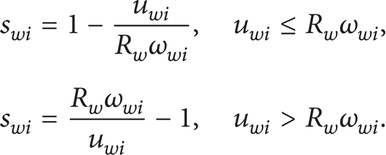
In the simulation of the vehicle dynamic response, the control performances are strongly depending on the precision and accuracy of tire forces. Longitudinal and lateral tire forces are calculated from the tire model. The popularly used tire models are “Dugoff tire model” [9], “Magic Formula” [10], “LuGre tire model” [11], and “Unitire” [12]. The Magic Formula tire model is a semiempirical model which is mathematically fitted to experimental data. The approach yields realistic tire behavior; it requires many experimental coefficients and is complicated. When the slip angle or the slip ratio is small, the longitudinal and lateral tire forces are linear to the tire deformation, and most normal driving conditions are in the linear region. The slops of the pure slip curves are defined as the longitudinal and lateral slip stiffness respectively. And when the slip angle or the slip ratio is larger than a certain value, the tire forces are saturated, and the slop tends to 0. So the paper proposed the piece-wise function to describe the tire model; it just needs a few coefficients. First the pure longitudinal and lateral sliding tire model is proposed, and then the combined working tire forces are calculated from the pure tire forces. The pure longitudinal and lateral slip working conditions could be fitted by using the piece-wise linear function

$F_x=F_x\left(s,F_z\right),\begin{array}{c}{F}_y=F_y\left(\alpha ,F_z\right),\end{array}$

(1)

where s is the slip ratio; α is the slip angle; and F _z is the vertical tire force.

The longitudinal wheel slip ratio for each individual tire is given by

$s_{wi}=\mathrm{1}-\frac{u_{wi}}{R_w{\omega }_{wi}},\hspace{1em}{u}_{wi}\le R_w{\omega }_{wi},s_{wi}=\frac{R_w{\omega }_{wi}}{u_{wi}}-\mathrm{1},\hspace{1em}{u}_{wi}>R_w{\omega }_{wi}.$

(2)

The calculation of the wheel longitudinal slip ratio and sideslip angle requires the wheel longitudinal speed. These wheel longitudinal speeds, considering the vehicle lateral dynamics, are calculated as

$u_{wfl}=\left(u-\frac{rB}{\mathrm{2}}\right)\cos \delta +\left(v+ar\right)\sin \delta ,\begin{array}{c}{u}_{wfr}=\left(u+\frac{rB}{\mathrm{2}}\right)\cos \delta +\left(v+ar\right)\sin \delta ,\\ u_{wrl}=\left(u-\frac{rB}{\mathrm{2}}\right),\\ u_{wrr}=\left(u+\frac{rB}{\mathrm{2}}\right).\end{array}$

(3)

The calculation of the wheel lateral slip angle requires the wheel lateral speed. These wheel lateral speeds are calculated as

$v_{wfl}=-\left(u-\frac{Br}{\mathrm{2}}\right)\sin {\delta }_{lf}+\left(v+ar\right)\cos \delta ,\begin{array}{c}{v}_{wfr}=-\left(u+\frac{Br}{\mathrm{2}}\right)\sin {\delta }_{rf}+\left(v+ar\right)\cos \delta ,\\ v_{wrl}=v-br,\\ v_{wrr}=v-br.\end{array}$

(4)

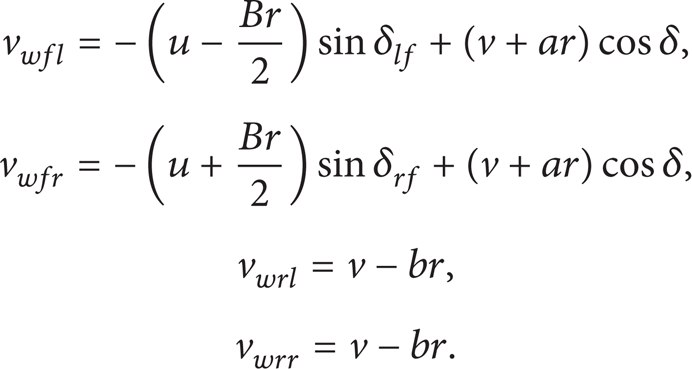
Assuming the small lateral velocity and yaw angular velocity, the slip angle can be approximately obtained by

${\alpha }_{fi}={\sigma }_f-\frac{u_{wfi}}{u_{wfi}},\hspace{1em}{\alpha }_{ri}=-\frac{v_{wrl}}{u_{wrl}}\hspace{1em}\left(i=l,r\right).$

(5)

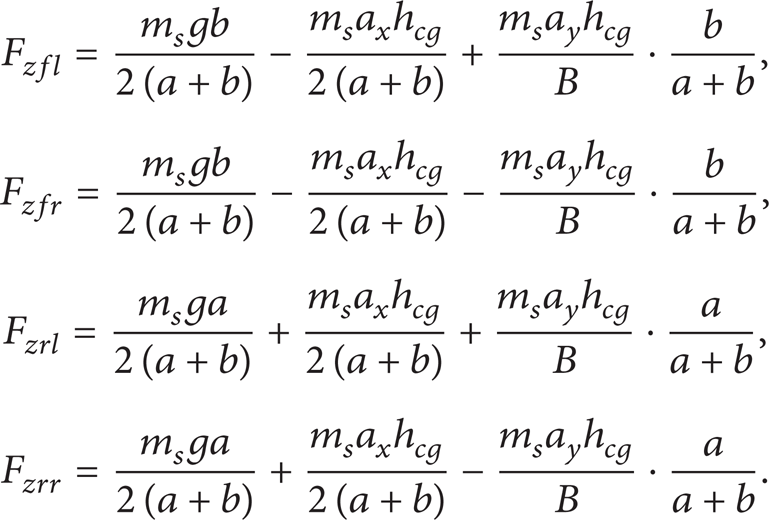
Considering the pitch load transfer and the roll load transfer is ignored, the normal forces F _z at the front and rear tires are calculated by

$F_{zfl}=\frac{m_{s}gb}{\mathrm{2}(a+b)}-\frac{m_s{a}_x{h}_{cg}}{\mathrm{2}\left(a+b\right)}+\frac{m_s{a}_y{h}_{cg}}{B}·\frac{b}{a+b},\begin{array}{c}{F}_{zfr}=\frac{m_{s}gb}{\mathrm{2}(a+b)}-\frac{m_s{a}_x{h}_{cg}}{\mathrm{2}\left(a+b\right)}-\frac{m_s{a}_y{h}_{cg}}{B}·\frac{b}{a+b},\\ F_{zrl}=\frac{m_{s}ga}{\mathrm{2}(a+b)}+\frac{m_s{a}_x{h}_{cg}}{\mathrm{2}(a+b)}+\frac{m_s{a}_y{h}_{cg}}{B}·\frac{a}{a+b},\\ F_{zrr}=\frac{m_{s}ga}{\mathrm{2}(a+b)}+\frac{m_s{a}_x{h}_{cg}}{\mathrm{2}(a+b)}-\frac{m_s{a}_y{h}_{cg}}{B}·\frac{a}{a+b}.\end{array}$

(6)

In the beginning, the longitudinal and lateral tire forces F_X0 and F_Y0 are calculated under the assumption that the tire is in pure longitudinal and lateral slip condition. The coupling slip condition is taken into account in second step.

2.1. Pure Longitudinal Slip

The longitudinal tire force F_X0 under the pure slip condition is calculated by

$F_{X\mathrm{0}}=\{\begin{array}{cc}{C}_x·s,\hfill & \left|s\right|<s_{\mathrm{1}},\hfill \\ C_x·s_{\mathrm{1}}·\mathrm{sgn}\left(s\right),\hfill & s_{\mathrm{1}}\le \left|s\right|<s_{\mathrm{2}},\hfill \\ [C_x·s_{\mathrm{1}}-\frac{C_x·s_{\mathrm{1}}-F_{\text{end}}}{s_{\mathrm{2}}-\mathrm{1}}\hfill & \hfill \\ \hspace{1em}·\left(\left|s\right|-s_{\mathrm{2}}\right)\phantom{\frac{C_x·s_{\mathrm{1}}-F_{\text{end}}}{s_{\mathrm{2}}-\mathrm{1}}}]·\mathrm{sgn}\left(s\right),\hfill & \left|s\right|>s_{\mathrm{2}}.\hfill \end{array}$

(7)

Here, s₁ = 7s_{1_nom}; C _x = C _{x nom} (1 + ((F _z -F_{z_nom})/F_{z_nom})); $s_{\mathrm{2}}=s_{{\mathrm{2}}_{\mathrm{nom}}}{(\mathrm{1}+((F_z-F_{z\_\mathrm{nom}})/{\mathrm{6}F}_{z\_\mathrm{nom}}))}^{-\mathrm{2}}$ F_end = ((F_{end_nom}/F_{z_nom}) + ((F _z -F_{z_nom})/4F_{z_nom}))^0.8μF _z ; F_{end_nom} = 3000(1 + ((F _z -F_{z_nom})/6F_{z_nom})).

2.2. Pure Lateral Slip

The lateral tire force F_Y0 under the pure slip condition is calculated by

$F_{Y\mathrm{0}}=\{\begin{array}{cc}-C_y·\alpha ,\hfill & \left|\alpha \right|<\mathrm{0.85}{\alpha }_{\mathrm{0}},\hfill \\ -\frac{C_y}{\mathrm{6}}·\left(\left|\alpha \right|+\mathrm{4.25}{\alpha }_{\mathrm{0}}\right)\hfill & \hfill \\ \hspace{1em}·\text{sng}\left(\alpha \right),\hfill & \mathrm{0.85}{\alpha }_{\mathrm{0}}\le \left|\alpha \right|<\mathrm{1.75}{\alpha }_{\mathrm{0}},\hfill \\ F_{\text{peak}}·\text{sng}\left(\alpha \right),\hfill & \left|\alpha \right|>\mathrm{1.75}{\alpha }_{\mathrm{0}}.\hfill \end{array}$

(8)

Here, $C_y=C_{y_{\mathrm{nom}}}(\mathrm{1}+(F_z/F_{z_{\mathrm{nom}}}))/\mathrm{2.5}$ $F_{\text{peak}}={(\mathrm{0.9}-\mathrm{0.182}((F_z/F_{z_{\mathrm{nom}}})-\mathrm{1}))}^{\mathrm{0.5}}$ α₀ = F_peak/C _y .

2.3. Combined Working Condition

The longitudinal and lateral tire forces in the combined driving and steering condition are given by [13]

${\delta }_x=-\frac{s}{s+\mathrm{1}},\hspace{1em}\hspace{1em}{\delta }_x^{*}=\frac{{\delta }_x}{{\delta }_{x\max }},\begin{array}{c}{\delta }_y=\frac{\tan \left(\alpha \right)}{s+\mathrm{1}},\hspace{1em}\hspace{1em}{\delta }_y^{*}=\frac{{\delta }_y}{{\delta }_{y\max }},\\ {\delta }_{\text{total}}=\sqrt{{\delta }_x^{\mathrm{2}}+{\delta }_y^{\mathrm{2}}},\hspace{1em}\hspace{1em}{\delta }_{\text{total}}^{*}=\sqrt{{\delta }_x^{*\mathrm{2}}+{\delta }_y^{*\mathrm{2}}},\\ s^{\prime }=\frac{{\delta }_{\text{total}}^{*}·{\delta }_{x\max }·\mathrm{sign}\left({\delta }_x\right)}{\mathrm{1}+{\delta }_{\text{total}}^{*}·{\delta }_{x\max }·\mathrm{sign}\left({\delta }_x\right)}·\frac{{\mu }_{\mathrm{0}}}{\mu },\\ {\alpha }^{\prime }=\arctan \left({\delta }_{\text{total}}^{*}·{\delta }_{y\max }·\mathrm{sign}\left({\delta }_x\right)\right)·\frac{{\mu }_{\mathrm{0}}}{\mu },\\ F_x=F_{x\mathrm{0}}·\mu ·\frac{{\delta }_x}{{\delta }_{\text{total}}}·\mathrm{sign}\left(s^{\prime }\right),\\ F_y=F_{y\mathrm{0}}·\mu ·\frac{{\delta }_y}{{\delta }_{\text{total}}}·\mathrm{sign}\left({\alpha }^{\prime }\right).\end{array}$

(9)

To well approach the Magic Formula tire model, in the linear region, the slope of the piece-wise linear tire model should be similar to the Magic Formula tire model; and in the saturation region, the results of the piece-wise tire model should be approximated to the Magic formulation model. And it should be suitable for the pure condition as well as the combined condition.

To validate the preciseness of the piece-wise linear tire model, the comparison results are plotted in Figures 1–4. Figures 1–2 show the comparison of Magic Formula tire forces and the piece-wise tire forces under different vertical forces. It can be found that during the pure longitudinal sliding and pure lateral sliding, the piece-wise linear tire model is accurate (piece-wise linear tire model parameters are shown in Table 1). Figures 3–4 show the comparison of Magic Formula tire forces and the piece-wise tire forces at different slip ratios and slip angles. There are still some errors compared with the Magic Formula tire model, especially when the slip angle or slip ratio is increasing, but it describes well the tire model and can be used in the estimation algorithm due to the small calculation load.

Table 1:

Piece-wise linear tire model parameters.

Nominal load	N o	4000 N
Nominal slip ratio 1	s 1_nom⁡	0.01
Nominal slip ratio 2	s 2_nom⁡	0.25
Nominal longitudinal stiffness	C x_nom	420000
Nominal lateral stiffness	C y_nom	1000 N/deg

Figure 1:

The longitudinal tire force for various vertical tire forces of 2 kN, 4 kN, 6 kN, and 8 kN.

Figure 2:

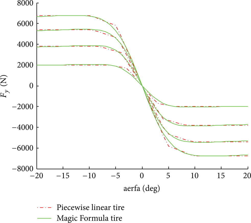
The lateral tire force for various vertical tire forces of 2 kN, 4 kN, 6 kN, and 8 kN.

Figure 3:

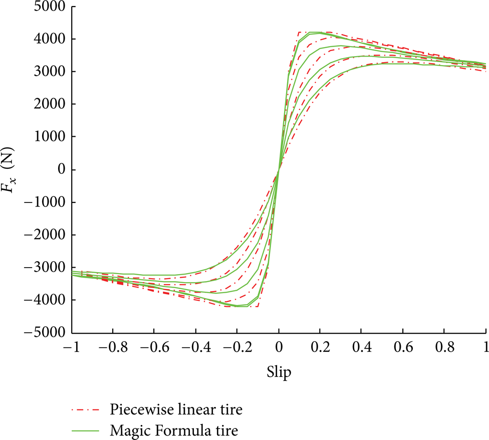
The longitudinal tire force for various slip angles of 0^°, 4^°, 8^°, 12^°, and 16^° (F _z = 4000 N).

Figure 4:

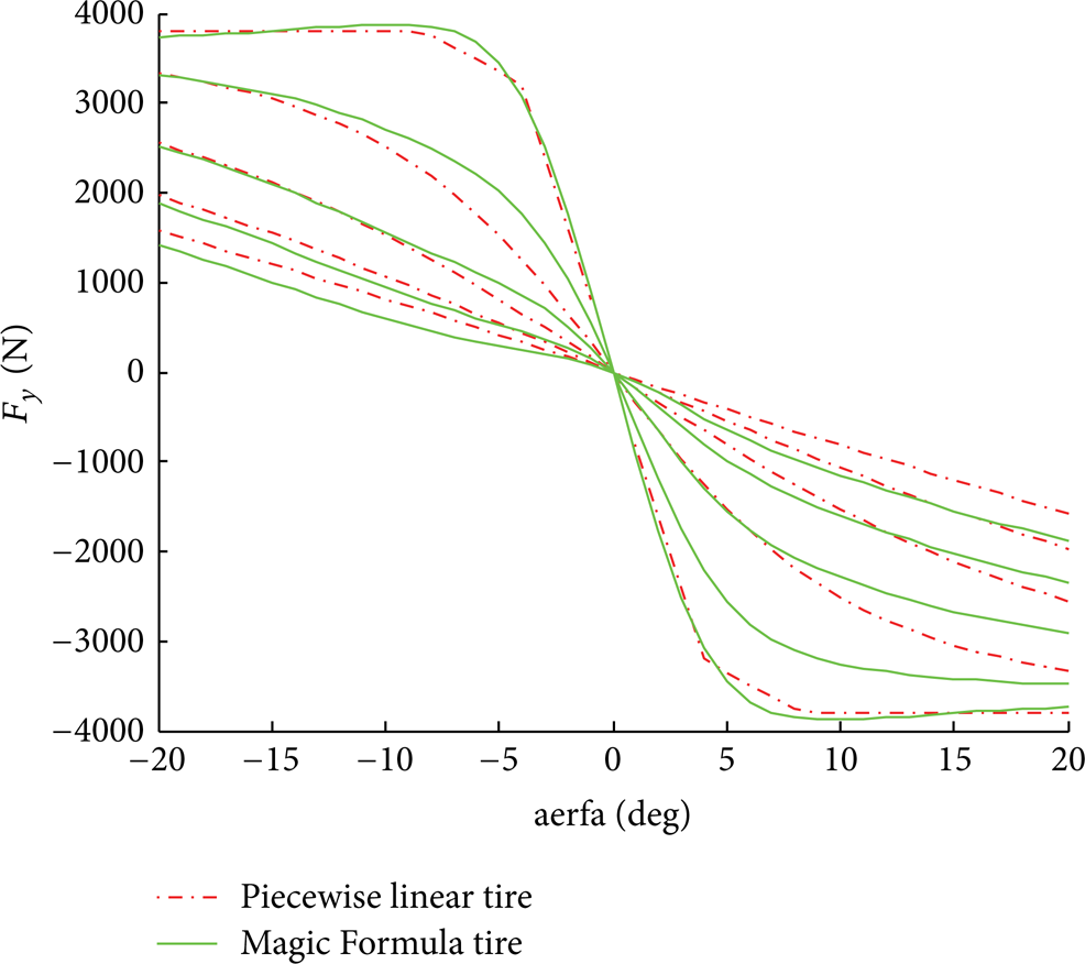
The lateral tire force for various slip ratios of 0, 0.2, 0.4, 0.6, and 0.8 (F _z = 4000 N).

3. Vehicle Model

Figure 5 shows the schematic of the vehicle model; it is 3DoF vehicle model, which consists of the longitudinal, the lateral, and the yaw motion, front wheel steering, and considering the load transfer, and the four-wheel spin speeds can be measured by the equipped sensors. In the paper, the subscripts of the individual wheels are list in Table 2. The vehicle dynamic equations can be described as follows [14]

$m\left(\dot{u}-vr\right)={\displaystyle \sum }{F}_{xi}^{}\hspace{1em}\left(i=fl,fr,rl,rr\right)\begin{array}{c}m\left(\dot{v}+ur\right)={\displaystyle \sum }{F}_{yi}^{}\hspace{1em}\left(i=fl,fr,rl,rr\right)\\ I_{zz}\dot{r}=\left[{\displaystyle \sum }_{i=lf,lr}{F}_{xi},{\displaystyle \sum }_{i=rf,rr}{F}_{xi},{\displaystyle \sum }_{i=lf,rf}{F}_{yi},{\displaystyle \sum }_{i=lr,rr}{F}_{yi}\right]\times {\left[-\frac{B_f}{\mathrm{2}},\frac{B_r}{\mathrm{2}},a,-b\right]}^{{\rm T}},\\ r=\dot{\psi },\end{array}$

(10)

where m = m _s + 2(m _uf + m _ur ); Ψ is the yaw angle. Consider

$a_x=\dot{u}-rv,\begin{array}{c}{a}_y=\dot{v}+ru,\end{array}$

(11)

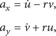
where a_x is the longitudinal acceleration; a_y is the lateral acceleration.

Table 2:

Abbreviations for the wheel positions.

fl	Front left	fr	Front right
rl	Rear left	rr	Rear right

Figure 5:

Schematic of the vehicle model.

The forces F _xi and F _yi can be computed by the longitudinal tire force F _wxi , lateral force F _wyi , and the steer angle δ, from the following equations:

$F_{xi}=F_{xwi}\cos {\delta }_i-F_{ywi}\sin {\delta }_i,F_{yi}=F_{xwi}\sin {\delta }_i+F_{ywi}\cos {\delta }_i,\phantom{\text{iiiiiiiiiiiiiiii}}\left(i=fl,fr,rl,rr\right),$

(12)

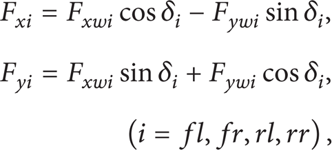
where front steering input δ _f = δ; δ _r = 0.

Based on (1)–(12), all presented submodels are merged into one model for the estimator design,

$\dot{x}\left(t\right)=f\left(x\left(t\right),u\left(t\right),w\left(t\right)\right),\begin{array}{c}y\left(t\right)=h\left(x\left(t\right),u\left(t\right),v\left(t\right)\right),\end{array}$

(13)

where state vector x = [v _x ,v _y ,r]′; the control input and measurement input u = [δ, w _fl ,w _fr ,w _rl ,w _rr ]′; the observations y = [a _x ,a _y ]′; w(t) is the process noise which is assumed to be drawn from a zero mean with covariance Q; and v(t) is the observation noise which is assumed to be zero mean Gaussian white noise with covariance of R.

Assuming the zero holds for the system input u(t) during the sampling time ΔT, the discrete form of the system could be obtained as follows:

$x\left(k+\mathrm{1}\right)=x\left(k\right)+\mathrm{\Delta }T·f\left(x\left(k\right),u\left(k\right),w\left(k\right)\right),\begin{array}{c}y\left(k\right)=h\left(x\left(k\right),u\left(k\right),v\left(k\right)\right),\end{array}$

(14)

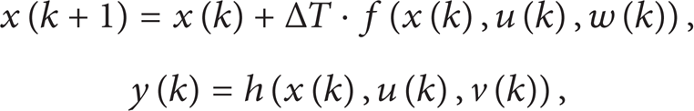
where k is the discrete time step.

4. Unscented Kalman Filter

Extend Kalman filter (EKF) is an optimal estimation method for the nonlinear systems. The nonlinear system is approximated to a linear system model around the last state estimate. It has been widely used in a number of nonlinear estimation and machine learning applications. These include estimating the state of a nonlinear dynamic system, parameters identification for nonlinear system, and dual estimation [15] where both states and parameters are estimated simultaneously. The EKF is based on the Taylor Expansion theory and first order approximation to linearize the nonlinear system. This [16] can introduce large errors in the true posterior mean and covariance, which may lead to suboptimal performance and sometimes divergence of the filter. And it is difficult to calculate the Jacobi matrix especially for the strong nonlinear system. For overcoming this defect, the unscented Kalman filter (UKF) [17] is proposed.

Unscented Kalman filter (UKF) [18] is based on the unscented transform (UT) theory and statistical linearization technique. This technique is used to linearize a nonlinear function of a random variable through a linear regression between n points drawn from the prior distribution of the random variable [19]. And the UKF uses the sigma points and could consider the high order terms during the state prediction and correction stage [20]. The UKF is better than the EKF in terms of robustness and speed of convergence [21]; the computational load in applying the UKF is comparable to the EKF. And the absence of the linearization error further allows us to execute the filter with lager sampling times. The UKF is as in Figure 6 and achieved by the following five steps.

Figure 6:

The block diagram of UKF.

(a) Sigma Points Calculation. In the paper, we use the symmetrical sampling method to pick up the sigma points. For the random variable state vector X, the mean is $\stackrel{-}{x}$ and the covariance of X is denoted by P ^x . The sigma points are chosen so that their mean and covariance are exactly $\stackrel{-}{x}$ and P ^x . Let X _k be a set of 2n + 1 sigma points (where n is the dimension of the state vector x),

$X_k=\{\begin{array}{cc}\stackrel{-}{x},\hfill & k=\mathrm{0},\hfill \\ \stackrel{-}{x}+{\left(\sqrt{\left(n+\lambda \right)P^x}\right)}_k,\hfill & k=\mathrm{1,2},\dots ,n,\hfill \\ \stackrel{-}{x}-{\left(\sqrt{\left(n+\lambda \right)P^x}\right)}_{k-n},\hfill & k=n+\mathrm{1},\dots ,\mathrm{2}n.\hfill \end{array}$

(15)

Here, λ = α²(n + κ)-n is a scaling parameter. The constant α determines the spread of the sigma around the $\stackrel{-}{x}$ and is usually set to a small value (1 ≤ α ≤ 10⁻⁴); κ≥0, which makes sure that the covariance matrix is positive definite.

(b) These Sigma Vectors Are Propagated through the Nonlinear System Function. Consider

$X_{k+\mathrm{1}}=X_{k+\mathrm{1}}+f\left(X_{k+\mathrm{1}},u_k,w_k\right)·\mathrm{\Delta }T.$

(16)

(c) Measurement Update. One has

$Y_{k+\mathrm{1}}=h\left(x_{k+\mathrm{1}},u_{k+\mathrm{1}},v_{k+\mathrm{1}}\right).$

(17)

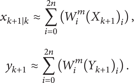
The mean of the state vector x_{k + 1} and the measurement value can be approximated by using a weighted sample of the sigma vectors as follows:

$x_{k+\mathrm{1}\mid k}\approx {\displaystyle \sum }_{i=\mathrm{0}}^{\mathrm{2}n}\left(W_i^m{\left(X_{k+\mathrm{1}}\right)}_i\right),\begin{array}{c}{y}_{k+\mathrm{1}}\approx {\displaystyle \sum }_{i=\mathrm{0}}^{\mathrm{2}n}\left(W_i^m{\left(Y_{k+\mathrm{1}}\right)}_i\right).\end{array}$

(18)

(d) Covariance Update. The covariance of the state vector and the measurement value can be calculated by

$P_{{\mathrm{\hspace{0.17em}\hspace{0.17em}}}^{k+\mathrm{1}\mid k}}^x={\displaystyle \sum }_{i=\mathrm{0}}^{\mathrm{2}n}\left[W_i^c\left({\left(X_{k+\mathrm{1}}\right)}_i-x_{k+\mathrm{1}}\right){\left({\left(X_{k+\mathrm{1}}\right)}_i-x_{k+\mathrm{1}}\right)}^{\prime }\right]+Q,\begin{array}{c}{P}_{k+\mathrm{1}}^y={\displaystyle \sum }_{i=\mathrm{0}}^{\mathrm{2}n}\left[W_i^c\left({\left(Y_{k+\mathrm{1}}\right)}_i-y_{k+\mathrm{1}}\right){\left({\left(Y_{k+\mathrm{1}}\right)}_i-y_{k+\mathrm{1}}\right)}^{\prime }\right]+R,\\ P_{k+\mathrm{1}}^{xy}={\displaystyle \sum }_{i=\mathrm{0}}^{\mathrm{2}n}\left[W_i^c\left({\left(X_{k+\mathrm{1}}\right)}_i-x_{k+\mathrm{1}}\right){\left({\left(Y_{k+\mathrm{1}}\right)}_i-y_{k+\mathrm{1}}\right)}^{\prime }\right].\end{array}$

(19)

The weight can be acquired by

$W_i^m=\left[\frac{\lambda }{\left(n+\lambda \right)},\underset{\mathrm{2}n}{\underbrace{\frac{\mathrm{1}}{\mathrm{2}/\left(n+\lambda \right)},\dots ,\frac{\mathrm{1}}{\mathrm{2}/\left(n+\lambda \right)}}}\right],\begin{array}{c}{W}_i^c=[\phantom{\underset{\mathrm{2}n}{\underbrace{\frac{\mathrm{1}}{\mathrm{2}/n+\lambda },\dots ,\frac{\mathrm{1}}{\mathrm{2}/n+\lambda }}}}\frac{\lambda }{\left(n+\lambda \right)}+\mathrm{1}-{\alpha }^{\mathrm{2}}+\beta ,\hspace{1em}\underset{\mathrm{2}n}{\underbrace{\frac{\mathrm{1}}{\mathrm{2}/(n+\lambda )},\dots ,\frac{\mathrm{1}}{\mathrm{2}/(n+\lambda )}}}].\end{array}$

(20)

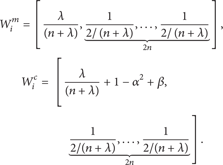
Here, assume that the system noise and the measurement noise are white Gaussian noise and covariance is Q and R respectively. β consider the high order moment of the prior distribution, for Gaussian distribution, β = 2 is optimal.

(e) Correction. Consider

$K_{k+\mathrm{1}}=P_{k+\mathrm{1}}^{xy}{\left(P_{k+\mathrm{1}}^y\right)}^{-\mathrm{1}},\begin{array}{c}{x}_{k+\mathrm{1}\mid k+\mathrm{1}}=x_{k+\mathrm{1}|k}+K_{k+\mathrm{1}}\left(z_{k+\mathrm{1}}-y_{k+\mathrm{1}}\right),\\ P_{k+\mathrm{1}\mid k+\mathrm{1}}^x=P_{k+\mathrm{1}\mid k}^x-K_{k+\mathrm{1}}{P}_{k+\mathrm{1}}^y{\left(K_{k+\mathrm{1}}\right)}^{\prime }.\end{array}$

(21)

Here, z_{k + 1} is the measurement value from the sensors, z = [a _x ,a _y ].

5. Simulation and Analysis

To validate the performance of the UKF estimator, the algorithm is implemented through cosimulation between Carsim software and MATLAB/Simulink software. Carsim is vehicle dynamics software widely used in the automotive industry. During the simulation, Carsim model is assumed to be a real vehicle due to its high accuracy; it provides the control inputs, measurement outputs, and the estimate state information as comparison values.

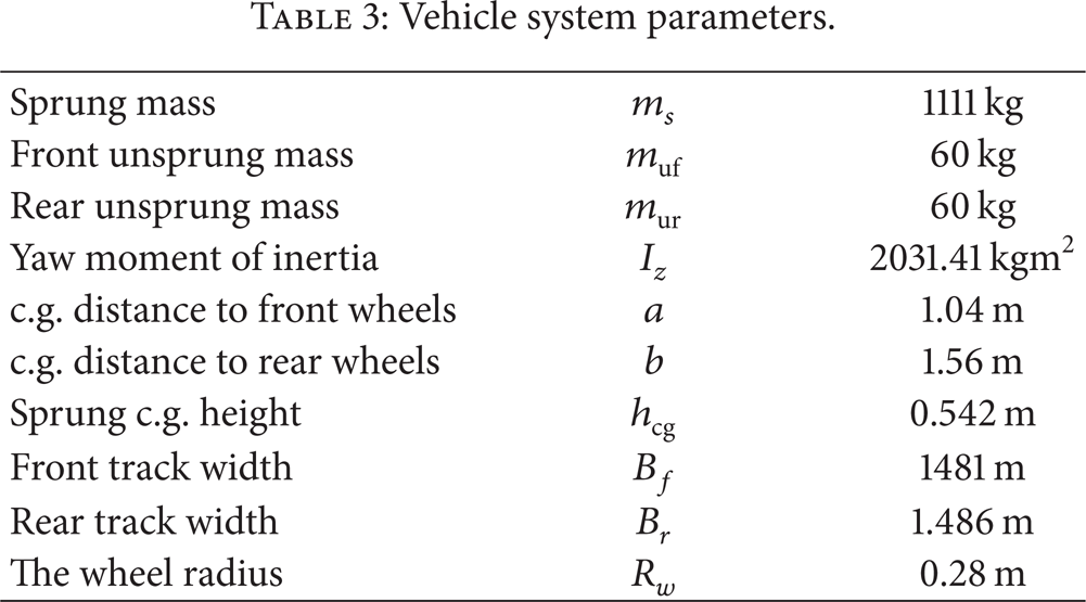
The simulation scenario includes two situations, the high road adhesion with high speed and the low road adhesion with low speed. The vehicle parameters are list in Table 3; and the ISO-3888/1 double line change (DLC) test is used in the simulation for validation of the proposed estimation algorithm. In the simulation, the estimation results of the Kalman filter with the linear tire model and the UKF with linear tire model are also presented as the comparison of the different estimation methods.

Table 3:

Vehicle system parameters.

Sprung mass	ms	1111 kg
Front unsprung mass	m uf	60 kg
Rear unsprung mass	m ur	60 kg
Yaw moment of inertia	I z	2031.41 kgm2
c.g. distance to front wheels	a	1.04 m
c.g. distance to rear wheels	b	1.56 m
Sprung c.g. height	h cg	0.542 m
Front track width	B f	1481 m
Rear track width	B r	1.486 m
The wheel radius	R w	0.28 m

5.1. High Road Adhesion Estimation

In the simulation, the initial velocity is 100 km/h, open loop throttle; and the tire-road friction coefficient is constant, 1. The front wheel steering input is plotted in Figure 7. The simulation results are presented in Figures 8–10.

Figure 7:

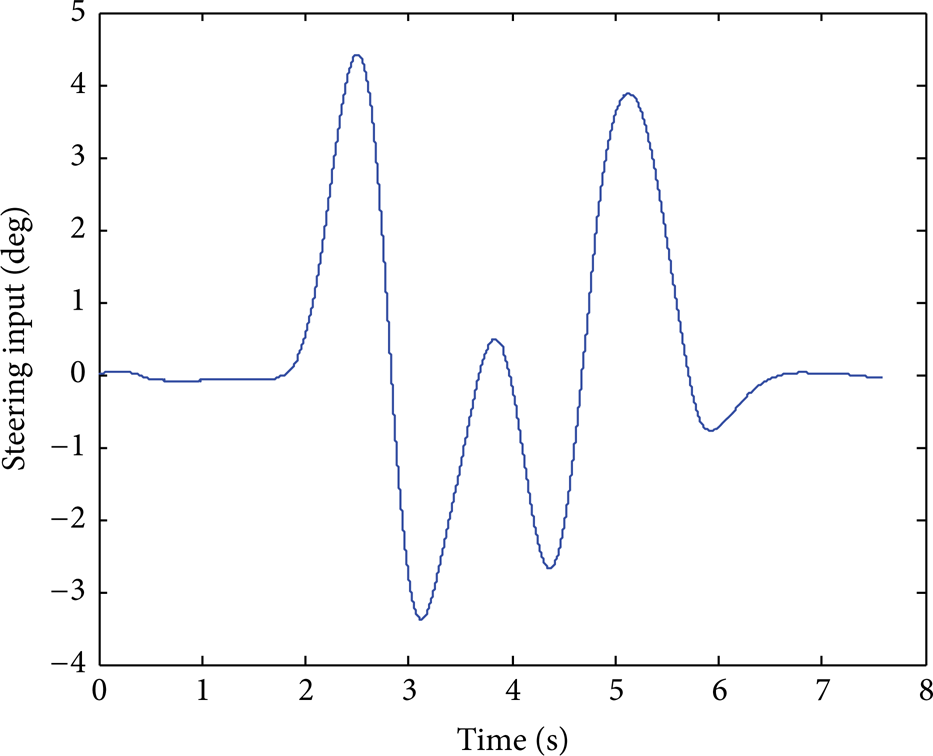
Steering angle input.

Figure 8:

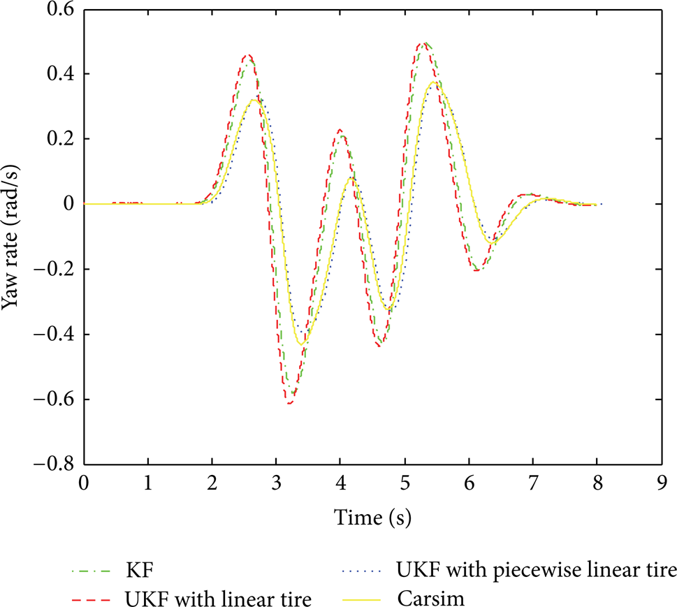
Yaw rate comparison.

Figure 9:

Lateral velocity comparison.

Figure 10:

Longitudinal velocity comparison.

Figures 8–10 show the yaw rate, lateral and longitudinal velocity estimation results using different estimation methods. It can be concluded that compared with the linear Kalman filter algorithm, the results of UKF estimator with the piece-wise linear tire model are more close to the real values. And during the estimation of the vehicle body lateral velocity, the UKF also has a big error when the lateral acceleration is bigger, as in Figure 9, because the 3DoF vehicle model does not consider the load transfer caused by the suspension motion.

Figure 11 shows the estimation results of tire slip angles (see Figure 11(a)) and the tire forces (see Figure 11(b)) of four individual wheels. It can be found that the UKF estimator can estimate the tire force well. We can also find that the estimation errors will increase when the lateral slip angle is large; these errors are partially due to the deficiency of the tire model. And performance of the tire model can be further improved by using the tire test data. From the above simulation results, it clearly indicates the effectiveness of the proposed UKF algorithm when vehicle is driving on high friction road.

Figure 11:

Slip angles estimation and lateral tire forces results of four wheels (the dotted line is UKF estimation results; continuous line is Carsim results).

5.2. Low Road Adhesion Estimation

The DLC test was then carried out on the low friction road; the initial velocity is 40 km/h, open loop throttle; and the tire-road friction coefficient is 0.2. The front wheel steering input is as in Figure 12; and the simulation results are as in Figures 13, 14, 15, and 16. The simulation results indicate that the UKF with the piece-wise linear tire can also have a good performance for the low road adhesion. It can be found that the UKF could estimate the vehicle state very well, even though the tire-road friction coefficient is very low. Figure 16 illustrates the estimated tire forces (see Figure 16(a)) and the tire kinemics (see Figure 16(b)) in comparison with the Carsim results. It can be concluded that the UKF could estimate the tire state information effectively under the low friction condition.

Figure 12:

Steering angle input.

Figure 13:

Yaw rate comparison.

Figure 14:

Lateral velocity comparison.

Figure 15:

Longitudinal velocity comparison.

Figure 16:

Slip angles estimation and lateral tire forces results of four wheels (the dotted line is UKF estimation results; continuous line is Carsim results).

From the above estimation results, it is obvious that performance of the UKF with the linear tire model is nearly the same as the Kalman filter based on the linear bicycle model, but the estimate performances are not good; the estimator errors are large, and these errors are mainly caused by the saturation tire forces; it means that during the linear region, the estimator's performance is good, but the estimation errors are increasing obviously during the nonlinear region.

6. Conclusion

1. The paper is based on the 3DoF vehicle model to estimate the vehicle state information which is necessary for the design of active safety controller, such as longitudinal velocity, lateral velocity, yaw rate and tire state information.

2. Considering the computation efficiency, the piece-wise linear tire model is proposed, and compared with the Magic Formula tire model, the simplified tire model is accurate.

3. According to the unscented transfer theory, combined with the Kalman filter, the UKF is presented to estimate the vehicle state information in real time.

4. Compared with the reference data from the Carsim, the estimation results of the vehicle state information are precise.

Conflict of Interests

The authors declare that there is no conflict of interests regarding the publication of this paper.