Numerical Simulation on Forced Convective Condensation of Steam Upward Flow in a Vertical Pipe

Abstract

A transient three-dimensional volume of fluid (VOF) simulation on condensation of upward flow of wet steam inside a 12 mm i.d. vertical pipe is presented. The effect of gravity and surface tension are taken into account. A uniform wall temperature has been fixed as boundary conditions. The mass flux is 130~6400 kg m⁻²'s⁻¹ and the turbulence inside the vapor phase and liquid phase have been handled by Reynolds stress model (RSM). The vapor quality of fluid is 0~0.4. The numerical simulation results show that, in all the simulation conditions, the bubbly flow, slug flow, churn flow, wispy annular flow, and annular flow are observed; in addition, the results of flow pattern are in good agreement with the regime map from Hewitt and Roberts. The typical velocity field characteristic of each flow pattern and the effect of velocity field on heat transfer of condensation are analyzed, indicating that the slug flow and churn flow have obvious local eddy. However, no obvious eddy is observed in other flow patterns and the streamlines are almost parallel to the flow direction. The simulation results of heat transfer coefficients and frictional pressure drop show good agreement with the correlations from existing literatures.

1. Introduction

Vertical pipes used in heat exchangers are very common. It is very important to calculate the heat transfer coefficient accurately for the design and optimization of heat exchangers, especially for the large-scale heat exchangers. However, when two-phase flows exist in vertical tubes, the calculation of heat transfer coefficient is very complex, mainly because of the presence of a vapor-liquid interface and different flow regimes and spatial distribution of the phases which has a very strong influence on heat transfer. Beside the development and validation of empirical correlations to predict global thermal performances, a more complete understanding and theoretical model of the two-phase flow and heat transfer process in vertical pipe are necessary for the design and optimization of heat exchangers.

Nowadays, the experimental research method is an important means of research for convective condensation because of its complexity. From an experimental point of view, a great wealth of studies have been carried out on the convective condensation in pipes. Local heat transfer coefficients of Isceon 59, R407C, and R404A, obtained from the measurement within a single smooth horizontal circular 3/8 copper tube, have been compared with the existing correlations for condensation heat transfer to assess the validity of these models for refrigerant mixtures by Boissieux et al. [1]. They found that the Dobson and Chato correlation [2] provided the best prediction for these refrigerant mixtures. The characteristics of condensation heat transfer and pressure drop for refrigerant R-134a flowing in a horizontal small circular pipe which has an inside diameter (i.d.) of 2 mm and the effects of the heat flux, mass flux, vapor quality, and saturation temperature of R-134a on the measured condensation heat transfer and pressure drop have been reported in Yan and Lin [3]. It was found that the condensation heat transfer coefficient is higher at a lower heat flux, at a lower saturation temperature, and at a higher mass flux. In addition, the measured pressure drop is higher for raising the mass flux but lower for raising the heat flux. An experimental investigation on heat transfer behavior during forced convection condensation inside a horizontal tube for wavy, semiannular, and annular flows has been published by Tandon et al. [4]. It shows that the nature of the relation for the heat transfer coefficient changes from annular and semiannular flow to wavy flow. Akers-Rosson correlations [5] with changed constant and power have been recommended for the two flow regimes. Col et al. [6] reported an experimental investigation of condensation of R134a inside a single square cross section minichannel when varying the channel orientation and found that the heat transfer coefficient is strongly affected by the relative importance of shear stress, gravity, and surface tension. Kim et al. [7] reported the condensation heat transfer coefficients of R-410A in flattened stainless tubes made from 5.0 mm inner diameter round tubes, and the test range covers saturation temperature 45°C, heat flux 10 kW m⁻², mass flux 100–400 kg m⁻²'s⁻¹, and quality 0.2–0.8. They observed that (1) the effect of aspect ratio on condensation heat transfer coefficient appears to be dependent on the flow pattern. For annular flow, the heat transfer coefficient increases as the aspect ratio increases. For stratified flow, however, reverse is true. (2) The pressure drop always increases as aspect ratio increases. (3) Round tube heat transfer correlations were not successful in predicting the flat tube heat transfer data. Experimental research was conducted to evaluate the heat transfer and friction characteristics of spirally corrugated tubes with 18/20 mm nominal diameters for the outer condensation of ammonia by Fernández-Seara and Uhía [8]. They found that the friction factors of corrugated tubes were 4–5 times higher than those of a smooth tube and the heat transfer performance of the corrugated tubes was around 1.27 times higher than the performance provided by smooth tubes. Gebauer et al. [9] investigated the condensation heat transfer of R134a and R290 on coated and uncoated horizontal smooth, standard finned, and high performance tubes by experiments and computational fluid dynamics (CFD-) simulations. It was found that, for the two refrigerants, the high performance tubes showed a larger bundle effect than the standard finned tubes and experimental results for coated tubes show a slightly lower heat transfer performance and no improvements of the condensate drainage could be observed for the modification. Lee et al. [10] examined condensation heat transfer in horizontal channels by testing two separate condensation modules using FC-72 as condensing fluid and water as coolant. The first module was dedicated to obtaining the detailed heat transfer measurements of the condensing flow and the second to video capture of the condensation film's interfacial behavior. Four dominant flow regimes are identified: smooth-annular, wavy-annular, stratified-wavy, and stratified.

Presently, it is difficult to study the flow and heat transfer characteristics of convective condensation with numerical simulation method, but some ideal results may be got by simplifying the model for some specific condensing condition. A volume of fluid (VOF) method was used by Kouhikamali [11] to simulate forced convective condensation in with the increase in the amount of inlet velocity and Reynolds number of inlet steam and the decrease in the temperature difference between the wall and saturated steam. An two-dimensional model for calculating film condensation of vapor flowing inside a vertical tube and between parallel plates is reported by Panday [12]. In the research, a methodology is presented to determine numerically the heat transfer coefficients, the film thickness, and the pressure drop. Turbulence in the vapor and condensate film is taken into account using mixing length turbulence models. Capillary blocking during condensation of water steam (m = 1.4 kg m⁻²'s⁻¹) in a 3 mm i.d. horizontal circular channel has been investigated numerically by means of the VOF method by Zhang et al. [13]; in their study, the flow both in vapor and liquid phase was laminar and the problem was treated as axisymmetrical, since gravity was considered negligible, while surface tension was assumed to be the dominant force. da Riva et al. [14–18] reported a series of extensive numerical simulations of condensation of R134a inside a 1 mm i.d. minichannel; a three-dimensional VOF model is adopted, while the effect of gravity and the importance of turbulence during condensation is analyzed. However, the above numerical simulation researches are only limited to the minichannels (i.e., 0.2 mm < D < 3 mm) and they referred to small range of vapor qualities and few types of flow patterns. In the meanwhile, very few numerical simulation researches on normal scale of pipe diameter (i.e., 6 mm < D < 20 mm) in industry (i.e., shell and tube heat exchangers, coil-wound heat exchangers, finned tube exchangers, and so on) and big range of vapor qualities and more types of flow patterns are carried out in existing literatures.

In the present work, a VOF model is adopted to simulate the heat transfer characteristics of forced convective condensation of steam upward flow in a vertical pipe. 15 typical working conditions are selected from the Hewitt flow regime map [19]. The range of mass flux and vapor quality of these working conditions is 130∼6400 kg m⁻²'s⁻¹ and 0∼0.4, respectively, including the following five kinds of flow pattern: bubbly flow, slug flow, churn flow, wispy annular flow, and annular flow. The research results may provide certain reference to the research in this field.

2. Numerical Simulation

A three-dimensional transient-state simulation of condensation of wet steam at pressure p = 5 Mpa, mass flux m = 130∼6400 kg m⁻²'s⁻¹, and vapor quality x = 0∼0.4 inside a 12 mm i.d. vertical pipe is proposed. The tube is 2 m long which consists of 1.8 m long section used to develop the velocity and temperature field, and the other 0.2 m long section used to observe the flow pattern and heat transfer. The Cartesian axis convention used here is shown in Figure 1 in which the ratio of X to Z axis is 200/12. Both the effects of gravity and surface tension have been taken into account. The present numerical procedure is implemented in a commercial package of Fluent. All the properties are considered to be pressure dependent and computed from the REFPROP8 database [23]. The pipe wall is held isothermal at a uniform temperature T _W = 535.09 K. The saturation temperature of the fluid is the function of local pressure and is limited in the range T _S = 537.09∼536 K to improve the calculation convergence. The assumption of constant wall temperature, instead of constant wall heat flux, is the closest one to the actual operation of condensers, since the condensing refrigerant must be cooled by means of a secondary fluid. The face between the developing section and the test section is held interior boundary condition. The mass flux boundary of liquid and vapor phase is imposed at the inlet according to each simulation condition, while an outflow boundary condition is imposed at the outlet. The liquid phase volume fraction α _L = 0 and velocity magnitude with zero are set to the initial condition. The mass flux boundary results in the uniform velocity and phase field at the inlet. As the calculation time goes on, the uniform velocity and phase field develop gradually to the actual velocity and phase field in the developing section, and then the fluid flows into the test section. Because of the transient of flow pattern, all parameters change with the time. When the time average values of wall heat flux, inlet and outlet pressure, and inlet and outlet vapor volume fraction are constant, the calculation proceeding is ended, and the flow pattern, heat transfer coefficient, and frictional pressure drop in the test section are observed and recorded.

Figure 1:

Cartesian axis convention (X to Z ratio is 200/12).

The case that vapor velocity is 8 m's⁻¹ and liquid velocity is 8 m's⁻¹ was selected to perform the mesh-independence test, because it has the strictest request to the mesh for its maximum mass flux. The present case was run both with a mesh displaying 630,000 hexahedral cells and a mesh displaying 980,000 cells and the difference in terms of computed heat transfer rate at the wall was around 0.7%, while the difference in terms of computed frictional pressure drop between the inlet and the outlet of the test section was around 1.8%. In order to accurately resolve the liquid film region and the vapor-liquid interface of the annular flow, the cell radial thickness in the near wall region is 0.1 mm, while the mesh is coarser in the core region (i.e., 0.5 mm) where the shear force between liquid and vapor is not large.

2.1. VOF Method

The VOF method [24, 25] is able to compute multiphase flows of immiscible fluids tracking the motion of the interface between them. A scalar field called “volume fraction” α representing the portion of the volume of the computational cell filled with one phase is used. Volume fractions of all phases sum to unity

${\alpha }_L+{\alpha }_G=1.$

(1)

The VOF algorithm is divided into two parts: a reconstruction step and a propagation step. The problem of interface reconstruction is that of finding an approximation to the section of the interface in each cut cell, by knowing the volume fraction in that cell and in the neighboring ones. Once the interface has been reconstructed, its motion by the underlying flow field is modeled by an advection algorithm. The implicit scheme was used in the simulation for time discretization, and the geometry reconstruction scheme was used for VOF calculations. The two-phase mixture was considered in the VOF method as a single fluid with properties changing depending on the value of the volume fraction α. The density ρ and the viscosity μ for a vapor-liquid mixture are locally computed for each cell by means of an arithmetic mean as follows:

$\begin{array}{c}\rho ={\rho }_L{\alpha }_L+{\rho }_G\left(1-{\alpha }_L\right),\\ \mu ={\mu }_L{\alpha }_L+{\mu }_G\left(1-{\alpha }_L\right).\end{array}$

(2)

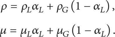
Thermal conductivity λ is also computed by means of an arithmetic mean as shown in the above equations. It must be noticed that some implementations of the VOF method adopt a geometric mean for the computation of viscosity; according to Boeck et al. [26], the arithmetic mean is optimal when the interface is perpendicular to the flow, while the harmonic mean is optimal when the interface is parallel.

The following continuity equations are solved:

$\begin{array}{c}\frac{\partial {\alpha }_L}{\partial t}+\nabla ·\left(\overrightarrow{u}{\alpha }_L\right)=\frac{S}{{\rho }_L},\\ \frac{\partial {\alpha }_G}{\partial t}+\nabla ·\left(\overrightarrow{u}{\alpha }_G\right)=-\frac{S}{{\rho }_G},\end{array}$

(3)

where S is the mass source term due to phase change. Regarding the momentum equation, the usual Navier-Stokes equations are used in the cells where only one of the two phases is present. At the interface (i.e., 0<α _L <1), instead, the force due to the surface tension, shown by the term ${\overrightarrow{F}}_{\sigma }$ in the following equation, must be taken into account:

$\frac{\partial \left(\rho \overrightarrow{u}\right)}{\partial t}+\nabla ·\left(\rho \overrightarrow{u}\overrightarrow{u}\right)=-\nabla p+\nabla ·\left[\left(\mu +{\mu }_t\right)\left(\nabla \overrightarrow{u}+\nabla {\overrightarrow{u}}^T\right)\right]+\rho \overrightarrow{g}+{\overrightarrow{F}}_{\sigma }.$

(4)

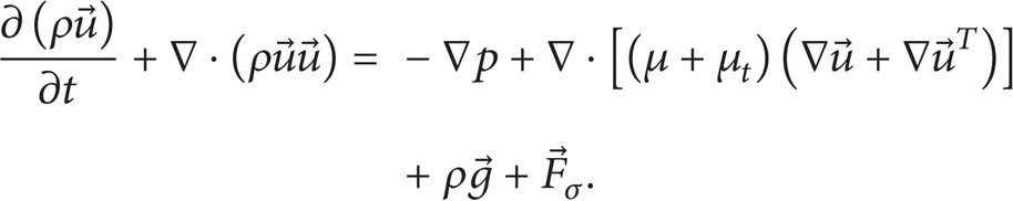
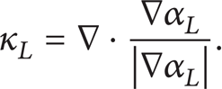
The effect of the surface tension is computed by means of the continuum surface force (CSF) model proposed by Brackbill [27]. The vapor-liquid interface is treated as a transition region of finite thickness and the effect of surface tension is modeled as a volume force. The surface normal is computed as the gradient of the volume fraction scalar; then, the surface curvature κ is obtained as the divergence of the normalized surface normal:

${\kappa }_L=\nabla ·\frac{\nabla {\alpha }_L}{\left|\nabla {\alpha }_L\right|}.$

(5)

The volumetric force in (4) due to the surface tension is finally computed as follows:

${\overrightarrow{F}}_{\sigma }={\sigma }_{LG}{\kappa }_L\nabla {\alpha }_L\frac{\rho }{\mathrm{0.5}\left({\rho }_L+{\rho }_G\right)}.$

(6)

All scalar values are shared by the phases throughout the domain, and thus no particular special treatment is needed for the energy or turbulence equations. The following energy equation is solved:

$\frac{\partial }{\partial t}\left(\rho h\right)+\nabla ·\left(\overrightarrow{u}\rho h\right)=\nabla ·\left({\lambda }_{\text{eff}}\nabla T\right)+h_{\text{LV}}S,$

(7)

where λ_eff is the effective thermal conductivity, h is the specific sensible enthalpy, and the last term (i.e., h_LVS) is the energy source due to phase change. The effective thermal conductivity is computed as follows:

${\lambda }_{\text{eff}}=\lambda +\frac{c_p{\mu }_t}{0.85}.$

(8)

The specific enthalpy is computed as a weighted average of liquid- and vapor-specific sensible enthalpies as follows:

$h=\frac{{\alpha }_L{\rho }_L{h}_L+{\alpha }_G{\rho }_G{h}_G}{{\alpha }_L{\rho }_L+{\alpha }_G{\rho }_G}.$

(9)

The same procedure is followed for the isobaric specific heat. The PRESTO! (PREssure STaggering Option) scheme was used in the simulation for the pressure interpolation, while the pressure-velocity coupling was handled by means of the PISO algorithm. The second upwind order scheme was used for the momentum equation, the turbulence equations, and the energy equation.

2.2. Turbulence Modeling

Anisotropy of turbulence around the vapor-liquid interface is obvious for the variation of interface and large difference of the physical properties between vapor and liquid phase. Therefore, Reynolds stress (RS) model [28–30] has been used in the present simulations because it can give good prediction for anisotropy turbulence flow:

$\underset{\text{Local}\mathrm{\hspace{0.17em}\hspace{0.17em}}\text{Time}\mathrm{\hspace{0.17em}\hspace{0.17em}}\text{Derivative}}{\underbrace{\frac{\partial }{\partial t}\left(\rho \overline{u_i^{\prime }{u}_j^{\prime }}\right)}}+\underset{C_{ij}}{\underbrace{\frac{\partial }{\partial x_k}\left(\rho u_k\overline{u_i^{\prime }{u}_j^{\prime }}\right)}}=\underset{D_{T,ij}}{\underbrace{-\frac{\partial }{\partial x_k}\left[\rho \overline{u_i^{\prime }{u}_j^{\prime }{u}_k^{\prime }}+\overline{p\left({\delta }_{kj}{u}_i^{\prime }+{\delta }_{ik}{u}_j^{\prime }\right)}\right]}}+\underset{D_{L,ij}}{\underbrace{\frac{\partial }{\partial x_k}\left[\mu \frac{\partial }{\partial x_k}\left(\overline{u_i^{\prime }{u}_j^{\prime }}\right)\right]}}\hspace{0.17em}\underset{P_{ij}}{\underbrace{-\rho \left(\overline{u_i^{\prime }{u}_k^{\prime }}\frac{\partial u_j}{\partial x_k}+\overline{u_j^{\prime }{u}_k^{\prime }}\frac{\partial u_i}{\partial x_k}\right)}}\times \underset{G_{ij}}{\underbrace{-\rho \beta \left(g_i\overline{u_j^{\prime }\theta }+g_j\overline{u_i^{\prime }\theta }\right)}}+\underset{{\Phi }_{ij}}{\underbrace{\overline{p\left(\frac{\partial u_i^{\prime }}{\partial x_j}+\frac{\partial u_j^{\prime }}{\partial x_i}\right)}}}-\underset{{\epsilon }_{ij}}{\underbrace{\mathrm{2}\mu \overline{\frac{\partial u_i^{\prime }}{\partial x_k}\frac{\partial u_j^{\prime }}{\partial x_k}}}}\times \underset{F_{ij}}{\underbrace{-\mathrm{2}\rho {\Omega }_k\left(\overline{u_j^{\prime }{u}_m^{\prime }}{\epsilon }_{ikm}+\overline{u_i^{\prime }{u}_m^{\prime }}{\epsilon }_{jkm}\right)}}+S_{\text{user}}.$

(10)

Of the various terms in these exact equations, C _ij , D_L,ij, P _ij , F _ij do not require any modeling. However, D_T,ij, G _ij , Φ _ij , ε _ij need to be modeled to close the equations.

D_T,ij can be modeled as follows [31]:

$D_{T,ij}=\frac{\partial }{\partial x_k}\left(\frac{{\mu }_t}{{\sigma }_k}\frac{\partial \overline{u_i^{\prime }{u}_j^{\prime }}}{\partial x_k}\right).$

(11)

The turbulent viscosity, μ _t , is computed similarly to the k-ε models as follows:

${\mu }_t=\rho C_{\mu }\frac{k^{\mathrm{2}}}{\epsilon },$

(12)

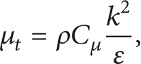
where C_μ = 0.09, k, and ε are modeled similarly to the k-ε models [23] as follows:

$\begin{array}{c}\frac{\partial }{\partial t}\left(\rho k\right)+\frac{\partial }{\partial x_i}\left(\rho k{u}_i\right)=\frac{\partial }{\partial x_j}\left[\left(\mu +\frac{{\mu }_t}{{\sigma }_k}\right)\frac{\partial k}{\partial x_j}\right]+\frac{\mathrm{1}}{\mathrm{2}}\left(P_{ii}+G_{ii}\right)-\rho \epsilon \left(\mathrm{1}+\mathrm{2}{M}_t^{\mathrm{2}}\right)+S_k,\\ \frac{\partial }{\partial t}\left(\rho \epsilon \right)+\frac{\partial }{\partial x_i}\left(\rho \epsilon u_i\right)=\frac{\partial }{\partial x_j}\left[\left(\mu +\frac{{\mu }_t}{{\sigma }_{\epsilon }}\right)\frac{\partial \epsilon }{\partial x_j}\right]\times C_{\epsilon \mathrm{1}}\frac{\mathrm{1}}{\mathrm{2}}\left(P_{ii}+C_{\epsilon \mathrm{3}}{G}_{ii}\right)\frac{\epsilon }{k}-C_{\epsilon \mathrm{2}}\rho \frac{{\epsilon }^{\mathrm{2}}}{k}+S_{\epsilon },\end{array}$

(13)

where σ _k = 0.82, σ_ε = 1.0, C_ε1 = 1.44, C_ε2 = 1.92, and C_ε3 is evaluated as a function of the local flow direction relative to the gravitational vector; S _k and S_ε are user defined source terms.

Φ _ij is modeled as the linear pressure-strain model [30], therefore,

${\Phi }_{ij}={\Phi }_{ij,\mathrm{1}}+{\Phi }_{ij,\mathrm{2}}+{\Phi }_{ij,w},$

(14)

where Φ_{ij, 1} is the slow pressure-strain term, which is modeled as

${\Phi }_{ij,\mathrm{1}}=-C_{\mathrm{1}}\rho \frac{\epsilon }{k}\left[\overline{u_i^{\prime }{u}_j^{\prime }}-\frac{\mathrm{2}}{\mathrm{3}}{\delta }_{ij}k\right]$

(15)

with C₁ = 1.8.

Φ_{ij, 2} is the rapid pressure-strain, which is modeled as

${\Phi }_{ij,\mathrm{2}}=-C_{\mathrm{2}}\left[\left(P_{ij}+F_{ij}+\frac{\mathrm{5}}{\mathrm{6}{G}_{ij}}-C_{ij}\right)-\frac{\mathrm{2}}{\mathrm{3}}{\delta }_{ij}\left(P+\frac{\mathrm{5}}{\mathrm{6}G}-C\right)\right],$

(16)

where C₂ = 0.6, P _ij ,F _ij ,G _ij , and C _ij are defined as in (10), P = 0.5P _kk , G = 0.5G _kk , and C = 0.5C _kk .

Φ_ij,w is wall-reflection term, which is modeled as

${\Phi }_{ij,w}=C_{\mathrm{1}}^{\prime }\frac{\epsilon }{k}\left(\overline{u_k^{\prime }{u}_m^{\prime }}{n}_k{n}_m{\delta }_{ij}-\frac{\mathrm{3}}{\mathrm{2}}\overline{u_i^{\prime }{u}_k^{\prime }}{n}_j{n}_k-\frac{\mathrm{3}}{\mathrm{2}}\overline{u_j^{\prime }{u}_k^{\prime }}{n}_i{n}_k\right)\times \frac{C_l{k}^{\mathrm{3}/\mathrm{2}}}{\epsilon d}+C_{\mathrm{2}}^{\prime }({\Phi }_{km,\mathrm{2}}{n}_k{n}_m{\delta }_{ij}-\frac{\mathrm{3}}{\mathrm{2}}{\Phi }_{ik,\mathrm{2}}{n}_j{n}_k-\frac{\mathrm{3}}{\mathrm{2}}{\Phi }_{jk,\mathrm{2}}{n}_i{n}_k)\frac{C_l{k}^{\mathrm{3}/\mathrm{2}}}{\epsilon d},$

(17)

where C₁′ = 0.5, C₂′ = 0.3, n_k is the x_k component of the unit normal to the wall, d is the normal distance to the wall, and C _l = C_μ^3/4/κ, where C_μ = 0.09 and κ is the von Kármán constant (= 0.4187).

G _ij is the production terms due to buoyancy, which are modeled as

$G_{ij}=-\frac{{\mu }_t}{\rho \text{P}{\text{r}}_t}\left(g_i\frac{\partial \rho }{\partial x_j}+g_j\frac{\partial \rho }{\partial x_i}\right),$

(18)

where Pr _t is the turbulent Prandtl number for energy, with a default value of 0.85.

The dissipation tensor ε _ij is modeled as

${\epsilon }_{ij}=\frac{\mathrm{2}}{\mathrm{3}{\delta }_{ij}\left(\rho \epsilon +\mathrm{2}\rho \epsilon \left(k/a^{\mathrm{2}}\right)\right)},$

(19)

where a is the speed of sound.

2.3. Phase Change Modeling

Phase change is not considered in the standard implementation of the VOF method [24, 25]; however, a number of different methods can be found in the literature. As an example, Welch and Wilson [32] modified the enhancement of the VOF method in order to directly calculate the discontinuous normal components of the heat flux at the interface and model heat and mass transfer.

In the present paper, the simpler numerical technique described by the following equations by Lee [33] has been used as follows:

$\begin{array}{c}S=-r{\alpha }_L{\rho }_L\frac{T-T_S}{T_S},\hspace{1em}T\ge T_S\\ S=r{\alpha }_G{\rho }_G\frac{T_S-T}{T_S},\hspace{1em}T<T_S,\end{array}$

(20)

where S is the source term in the continuity equations (3) and in the energy equation (7), T is the cell temperature and r is a positive numerical coefficient. In the case of condensation of a pure fluid, the interfacial temperature can be assumed to be equal to the saturation temperature. The above equations describe a simple numerical technique to impose this assumption as boundary condition. An example of adoption of Lee's equations [33] together with the VOF methods to model boiling flows can be found in Yang et al. [34]. A similar numerical technique to impose the saturation temperature as boundary condition at the interface can be found in Zhang et al. [13]. If at a certain computational step the temperature of a cell in the domain is higher than the saturation temperature, the first of the two equations is used; if this cell belongs to the vapor phase (i.e., α _L = 0), no mass transfer is computed; if this cell belongs to the liquid phase (i.e., α _L >0), mass transfer from the liquid to the vapor phase is computed. Besides, the temperature of the cell is decreased by the source term h_LVS in the energy equation (7). The computation is analogous for the cells with temperature lower than the saturation one. In this way, the presence of cells in the vapor phase with temperature lower than the saturation temperature is avoided, as well as the presence of cells in the liquid phase with temperature higher than the saturation temperature. The source term S is arbitrarily fixed; however, mass, momentum, and energy are conserved at every computational step. At convergence, interface reaches the saturation temperature, while cells inside the liquid phase reach a lower temperature and cells inside the vapor phase a higher temperature. In practice, the interfacial temperature obtained at convergence will not be exactly the saturation temperature. Excessively small values of the coefficient r lead to a significant deviation between the interfacial and saturation temperatures. Furthermore, when higher values of the coefficient r are used, the interface (i.e., the region of cells with 0<α _L <1) is sharper and thinner. However, too large values of r cause numerical convergence problems. In the present work, the coefficient r = 10000's⁻¹ was used in (20). The optimal values for the coefficient r strongly depend on the particular problem under solution and suitable values should be found for each case. As an example, Yang et al. [34] performed VOF simulation of boiling in a coiled tube using the value r = 100 s⁻¹.

3. Results and Discussion

All simulation conditions of this work are shown in Table 1, whose location in Hewitt and Roberts [19] flow regime map can be seen in Figure 2.

Table 1:

Simulated conditions.

Condition number	Vapor superficial velocity (m's−1)	Liquid superficial velocity (m's−1)
1	15.2	0.8
2	7.2	0.8
3	3.2	0.8
4	7.2	1.8
5	4	4
6	8	8
7	1.6	4.8
8	0.64	7.36
9	0.4	0.8
10	0.64	0.96
11	0.04	0.16
12	0.042	0.8
13	0.64	0.16
14	0.24	0.16
15	1.6	0.8

Figure 2:

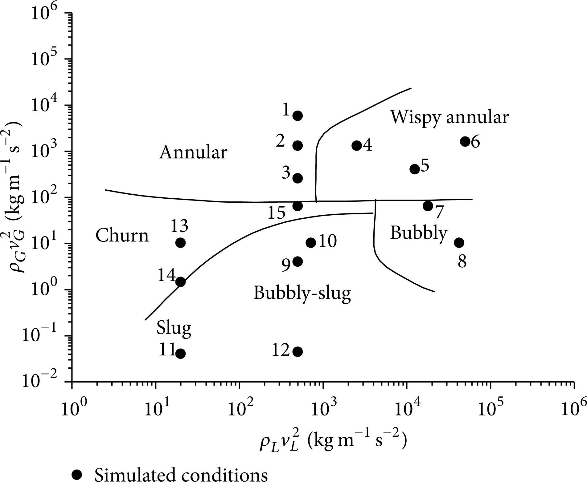
Distribution of simulated conditions in Hewitt and Roberts [19] flow regime map.

In order to verify the accuracy of simulation results, Boyko-Kruzhilin's correlation [20] is adopted to compare with the simulated heat transfer coefficients. Baker's correlation [21] is adopted to compare with the simulated frictional pressure drop of annular flows, while Dukler et al.'s correlation [22] is adopted to compare with the simulated frictional pressure drop of nonannular flows. The verification of simulations can be concluded from Figures 3 and 4. The heat transfer coefficient deviation of most cases is within ± 25%, while the deviation of frictional pressure drop shows the similar result. The deviations are arguably acceptable due to the complexity of two-phase flow.

Figure 3:

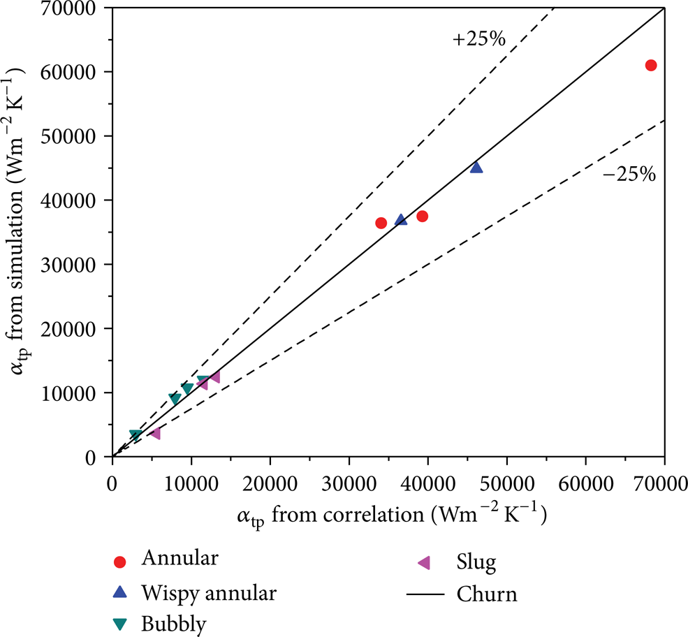
Heat transfer coefficient comparison between VOF simulation and Boyko-Kruzhilin [20] correlation.

Figure 4:

Frictional pressure drop comparison between VOF simulation and Baker's correlation [21] and Dukler et al.'s correlation [22].

The main flow pattern predicted from the simulation results of this work is bubbly, slug, churn, wispy annular, and annular, as shown in Figures 5–9. Table 2 presents the comparison between the flow pattern results predicted from this work simulation and Hewitt and Roberts [19] flow regime map. It can be seen that most of simulation results agree well with Hewitt and Roberts [19] flow regime map and the few inconsistent conditions occur around the transition line of flow patterns. Actually flow pattern transition is not a line but a zone, and, therefore, the simulation results are in good agreement with Hewitt and Roberts [19] flow pattern on the whole. The verification results of flow pattern, heat transfer coefficient, and fictional pressure drop all verify the accuracy of calculation model of this work.

Table 2:

Comparison between VOF simulation and Hewitt and Roberts [19] flow regime map.

No.	Flow patterns from Hewitt regime map	Flow patterns from simulation	Agreement or not
1	Annular	Annular	Yes
2	Annular	Annular	Yes
3	Annular	Wispy Annular	No
4	Wispy Annular	Wispy Annular	Yes
5	Wispy Annular	Wispy Annular	Yes
6	Wispy Annular	Wispy Annular	Yes
7	Bubbly	Bubbly	Yes
8	Bubbly	Bubbly	Yes
9	Bubbly-Slug	Bubbly-Slug	Yes
10	Bubbly-Slug	Bubbly-Slug	Yes
11	Slug	Slug	Yes
12	Slug	Slug	Yes
13	Churn	Churn	Yes
14	Churn	Slug	No
15	Churn	Churn	Yes

Figure 5:

Flow and temperature fields of bubbly flow (case 8: u _L = 7.36 m s⁻¹, u _G = 0.64 m s⁻¹, t = 0.65's).

Figure 6:

Flow and temperature fields of slug flow (case 14: u _L = 0.16 m s⁻¹, u _G = 0.24 m s⁻¹, t = 8.21's).

Figure 7:

Flow and temperature fields of churn flow (case 13: u _L = 0.16 m s⁻¹, u _G = 0.64 m s⁻¹, t = 2.13's).

Figure 8:

Flow and temperature fields of wispy annular flow (case 6: u _L = 8 m s⁻¹, u _G = 8 m s⁻¹, t = 0.24's).

Figure 9:

Flow and temperature fields of annular flow (case 3: u _L = 0.8 m s⁻¹, u _G = 3.2 m s⁻¹, t = 1.36's).

The typical flow field and temperature field of bubbly flow are shown in Figure 5. It can be seen from Figure 5(b) that streamlines of bubbly flow are straight and parallel with flow direction. The whole velocity field is similar to that of single phase. Figure 5(c) shows that the whole temperature field is nonsymmetry along the Z axis and the high temperature turns up in the bubble zone, which is different from single liquid phase. The gradient of temperature difference in the radial direction is larger than that in the single liquid phase, which results in larger heat transfer coefficient. As shown above, tiny bubbles in bubbly flow have no obvious influence on the flow but certain influence on the temperature field.

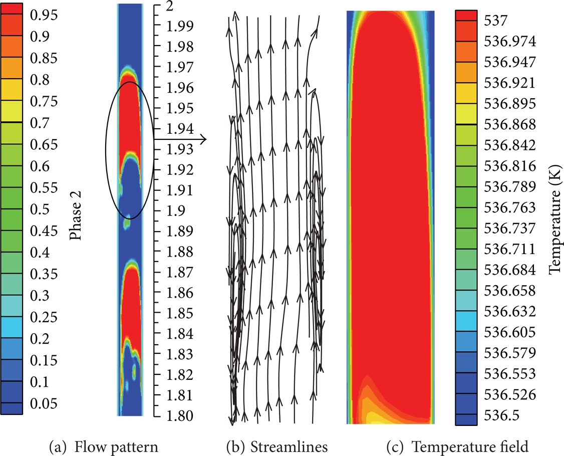
The typical flow field and temperature field of slug flow are shown in Figure 6. It can be seen from Figure 6(b) that streamlines of slug flow are crooked and nonuniform along the flow direction and there is obvious backflow in the gap between slug gas and pipe wall. Due to the backflow, the tail of slug gas is not smooth but has a trailing along the wall. However, there is no similar phenomenon in bubby flow because small diameter of bubbly flow leads to small buoyancy force and velocity slip, and the simulation modeling in this work cannot express this tiny interaction. On the contrary, the slug gas of slug flow is bulky and it is imposed on great buoyancy force, so the velocity slip is rather large, and the cavitation in the tail of slug gas causes negative pressure that leads to backflow. Figure 6(c) shows that the whole temperature field is nonuniform and heat transfer temperature difference varies in different zones, and the maximum temperature gradient exists in the liquid film of the backflow zone. As analyzed above, slug gas has significant impact on the flow and temperature field, especially enhancing heat transfer near the slug gas.

The typical flow field and temperature field of churn flow is shown in Figure 7. It can be seen from Figure 7(b) that streamlines of churn flow are crooked as wave, even backflow is turned up, along the flow direction, and the streamlines are neither parallel nor uniform. Due to the significant influence of vapor-liquid interaction, vapor phase and liquid phase have no regular shape. Figure 7(c) shows that the temperature field is irregular that is caused by the disordered velocity field. As analyzed above, flow field of churn flow is disturbed violently, which has significant impact on enhancing heat transfer.

The typical flow field and temperature field of wispy annular flow are shown in Figure 8. It can be seen Figure 8(b) that streamlines of wispy annular flow are approximately linear and uniform along the flow direction. Figure 8(c) shows that the whole temperature field of wispy annular flow is nonsymmetry along the Z axis and the obvious temperature boundary exists near the interface of gas and liquid. The temperature gradient is small in the main liquid film but is very large near the wall, which indicates very strong heat transfer in the liquid film. As analyzed above, the shear force between gas core and liquid film of wall has significant impact on enhancing heat transfer.

The typical flow field and temperature field of annular flow are shown in Figure 9, whose temperature field and velocity field are similar to wispy annular flow, and the difference of them is that annular flow has larger temperature gradient in the film near the wall, which indicates stronger heat transfer in the liquid film. Therefore, annular is a more ideal flow pattern for heat transfer.

4. Conclusions

In this work, three-dimensional transient-state VOF model and RSM turbulence model are used to simulate the characteristics of heat transfer and flow during the condensation process of wet steam upward flow in a vertical pipe. The influence of gravity and surface tension are taken into account. The inside diameter of simulated tube is 12 mm and the range of mass flux and vapor quality is 130∼6400 kg m⁻² s⁻¹ and 0∼0.4, respectively. The results of simulated heat transfer coefficient are in good agreement with Boyko-Kruzhilin [20] correlation, and the results of simulated frictional pressure drop are in good agreement with Baker's correlation [21] for annular flows and Dukler et al.'s correlation [22] for nonannular flows. The main flow patterns in the simulation conditions are bubbly, slug, churn, wispy annular, and annular, respectively. The simulation results agree well with Hewitt and Roberts [19] flow regime map, which illustrates that the results of this work are reliable.

After analyzing temperature field and flow field of each flow pattern, the important conclusions can be drawn as follows.

1. For bubbly flow, the velocity field of bubbly flow is similar to that of single phase flow, indicating that the interaction force between vapor and liquid phase is weak. But the temperature field is different from that of single phase.

2. For slug flow, there is obvious backflow in the liquid gap between slug gas and pipe wall; slug gas has significant impact on the flow field and temperature field near the slug gas.

3. For churn flow, the velocity field and temperature field are irregular and there is obvious velocity gradient near the vapor-liquid interface. It shows that flow field is disturbed violently in churn flow, which has significant impact on enhancing heat transfer.

4. The character of wispy annular flow is similar to annular flow. For wispy annular flow and annular flow, the liquid film near the wall is thin and impacted strongly by central gas core, which has significant impact on enhancing heat transfer.