Sage Journals: Discover world-class research

Abstract

The hybrid flow shop (HFS) problem is solved in this study through composite dispatching rules (CDRs) generated automatically. CDR is a simple approach to solve the HFS problem rapidly and easily. Genetic programming (GP) is the most common methodology to generate CDRs to solve combinational optimization problems. The disruption in the main operations of GP, such as crossover and mutation, is high. Scatter programming is proposed in this paper to generate CDRs with improved scalability and flexibility for HFS problems. The proposed algorithm includes a novel local improvement method, one-point traversal shaking search, to accelerate convergence. Simulation studies demonstrate that the proposed algorithm outperforms genetic programming and scatter programming with shaking. The dispatching rules generated automatically can also be reused in similar instances and yield better results than existing dispatching rules. The rate of convergence of the proposed algorithm is higher than that of scatter programming with shaking.

1. Introduction

The flow shop scheduling problem is a classic problem in production scheduling. In the flow shop scheduling problem, a set of jobs are processed in a series of stages in the same machine order, and each stage consists of only one machine. Hybrid flow shop (HFS) is an extension of the flow shop. In HFS, multiple machines operate in parallel in each stage. At least one stage involves more than one machine. The number of stages is more than 1. All jobs must follow the same production flow. Each job is processed on one machine in each stage. The number of jobs being operated at any time must be smaller than the number of machines in all stages. The number of stages is unlimited in HFS. However, as a complex combinational optimal problem, the HFS problem is NP-hard even if the number of stages is 2 [1].

Many approaches have been proposed to solve HFS problems. Branch and bound [2] is an exact algorithm to solve small instances of the HFS problem. However, the computational cost is comparatively high when this algorithm is utilized to solve medium and large instances of the HFS problem. Metaheuristics, such as tabu search [3], simulated annealing [4], and genetic algorithms [5], are nonexact approaches for job scheduling. Metaheuristics can obtain solutions for the HFS problem more efficiently than branch and bound. However, the computational cost of metaheuristics for the HFS problem is also large when the instance of the HFS problem is large. Dispatching rules are deterministic heuristics utilized to solve the HFS problem. The computation time of dispatching rules is small, and the implementation of the dispatching rules is easy. Therefore, dispatching rules are widely used to solve the HFS problem although the quality of the solutions obtained by dispatching rules may not be as good as that obtained by branch and bound and metaheuristics. Dispatching rules employ different formulae to calculate priorities for unscheduled jobs. When one machine is idle, the job with the highest priority is selected and operated on this idle machine. Dispatching rules are usually constructed by domain experts. Genetic programming [6] (GP) has been recently applied to obtain dispatching rules automatically for production scheduling problems. However, in GP, the disruption in the main operations, such as crossover and mutation, is high.

An automatic heuristic generation method with scatter programming [7] (SP) is developed in this paper for the HFS problem. The main operators of SP, such as children generation and local improvement methods, are utilized to balance intensification and diversification. A new local improvement method, one-point shaking, is introduced to improve the rate of convergence. Simulation studies conducted on HFS benchmark instances demonstrate that the proposed algorithm outperforms GP. The generated dispatching rules yield good results and can be potentially reused in new problem instances. The local improvement method proposed in this study can improve the rate of convergence of the algorithm.

The rest of the paper is organized as follows. Section 2 provides a formal definition of the HFS problem. Section 3 highlights several relevant studies related to dispatching rules for solving HFS problems and two metaheuristic programming approaches, GP and SP. Section 4 describes the representation of the solution in SP. An SP approach for solving the HFS problem is presented in Section 5. Section 6 presents the simulation results for a set of HFS benchmark instances. Lastly, Section 7 presents the conclusions and discussion on future work.

2. Formulation of the HFS Problem

In HFS, the parameters and decision variables utilized in the formulation are described as follows.

p_js is the processing time of job j.

c_js is the complete time of job j at stage s.

X is the binary variable that indicates whether a job is operating in the specified machine or not. X_jsm = 1 if job j operates at stage s in machine m; otherwise, X_jsm = 0.

Y is the binary variable that indicates whether one job operates before another job at one stage. If job i operates before j at stage s, Y_ijs = 1; otherwise, Y_ijs = 0.

The number of jobs is n, and the number of stages is q. The model of the HFS problem is

\min (\max c_{j q}), \forall j,

(1)

\sum_{m = 1} X_{j s m} = 1,

(2)

c_{j s} - c_{j, s - 1} \geq \sum_{l = 1} X_{j s m} p_{j s},

(3)

c_{i s} - c_{j s} - p_{i s} \geq - M (Y_{i j s} - X_{i s m} - X_{j s m} + 2),

(4)

c_{j s} - c_{i s} - p_{j s} \geq M (Y_{i j s} + X_{i s m} + X_{j s m} - 3) .

(5)

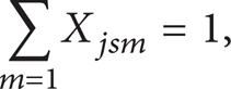
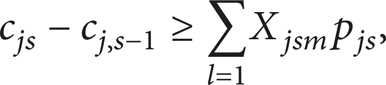
M is a sufficiently large number. The objective of HFS in this study is to minimize makespan, which indicates the maximum completion time of the last operation on the last machine. Constraint (2) stipulates that, at any time, one job can only operate in only one machine. Constraint (3) states that the operation of job j at stage s cannot begin before its release from the previous stage. Constraints (4) and (5) guarantee that, for all machines, any other job cannot start operating in a machine when this machine has not finished operating its job.

3. Related Work

3.1. Dispatching Rules for HFS

Dispatching rules are utilized as simple heuristics for the HFS problem. Dispatching rules can be applied to obtain a priority score for each candidate job waiting to be processed on machines. When a machine is idle, the job with the highest priority score is selected and processed on this machine.

Dispatching rules are of two types: simple dispatching rules (SDRs) and composite dispatching rules (CDRs). SDR usually contains only one parameter, such as release time or due date. For example, the earliest release time is an SDR. When a machine is idle, the unscheduled job with the earliest release time is selected and processed on this machine. SDR does not perform well in different instances or objective functions of the HFS problem because the parameter of SDR is limited. CDR involves a formula to calculate a priority score for each unscheduled job. A formula contains one or more parameters to combine the good features of SDRs. CDRs are usually constructed through human experience. Researchers have recently focused on how to automatically generate a CDR based on SDRs for an instance of scheduling problems.

3.2. GP

As a population-based evolutionary algorithm, GP is the most common method to generate CDR automatically. GP is based on a genetic algorithm (GA) and obtains new individuals by selection, crossover, and mutation. GP employs tree-based encoding. The tree-based formula consists of two sets of elements, namely, parameters and mathematical operators. For a production scheduling problem, GP produces a dispatching rule to calculate a priority score for an operation. The operation with the highest priority will be selected for processing.

GP has been employed to solve production scheduling problems. Dimopoulos and Zalzala [8] were the first to apply GP to solve a classic one-machine scheduling problem. The dispatching rules obtained by traditional GP performed well not only in the training set but also in new instances of the problem. In 2006, Geiger et al. [9] extended the work of Dimopoulos and Zalzala and proposed an autonomous learning approach based on GP to obtain dispatching rules whose performance is better than that of other existing dispatching rules. Jakobović et al. [10] employed GP to solve a parallel machine scheduling problem in 2007. Tay and Ho [11] applied GP to derive dispatching rules for solving multiobjective flexible job-shop problems.

The disruption of the main operations of GP is high. Therefore, the rate of GP is low. SP was proposed to overcome this drawback.

3.3. SP

SP is another metaheuristic programming approach based on the scatter search (SS) algorithm [12]. SS is a population-based metaheuristic that achieves balance between intensification and diversification. SS employs a reference set (Ref-Set) to maintain solutions in the operation process. The solutions selected from Ref-Set are placed in Sub-Set. Then, new solutions are combined with the solutions in Sub-Set andimproved via a local improvement method. Finally, Ref-Set is updated by the improved solutions. In 2010, Hedar and Osman [7] proposed SP to solve machine learning problems with three tree-based local search methods, namely, shaking search, grafting search, and pruning search. Shaking search selects some nodes of the tree and replaces them with random ones. Grafting search changes the tree structure and replaces some leaf nodes in the tree with branches generated randomly. Pruning search does not add any branches to the tree but cuts some branches from the tree and replaces them with leaf nodes generated randomly. The experimental results in [7] show that SP is stable and effective in solving machine learning problems. However, the disruption of the three local improvement methods is also high. In the present study, a novel local improvement is proposed to improve the convergence rate of SP.

4. Solution Representation

SP employs tree-based encoding with dynamic length to represent a solution. Therefore, SP is unsuitable for encoding solutions directly to production scheduling problems, such as the HFS problem. However, SP is suitable for encoding a formula of dispatching rules to solve HFS. Two types of parameters, namely, terminal and function sets, can be utilized to code dispatching rules as solutions in SP.

4.1. Terminal Set

Many parameters can influence job scheduling of the HFS problem in different dispatching rules. In this study, the terminal set includes the following five parameters to form dispatching rules for the HFS problem.

r_i is the release time for job i.

p_is is the processing time for job i at stage s.

d_i is the due date for job i.

w_i is the work remaining for job i.

T is the current time.

These parameters were derived from 13 dispatching rules in [13, 14]. Different parameters might generate different effects on results.

4.2. Function Set

The combination of parameters in the terminal set plays an important role in the performance of the dispatching rule. The function set contains six basic mathematical operators: addition (+), subtraction (−), multiplication (*), division (/), maximum (max), and minimum (min). All of these mathematical operators have two input parameters and one return value. The return value of the division operator is set to 1 when the value of the denominator is equal to 0. Mathematical operators cannot be leaf nodes in tree-based dispatching rules.

An example of a tree-based dispatching rule is shown in Figure 1. The tree is interpreted in a depth-first, left to right way. The dispatching rule contains two parameters (d_i and r_i) of the terminal set and three mathematical operators, namely, addition (+), subtraction (−), and division (/). The formula represented in Figure 1 is (d_i/r_i) − (d_i + d_i).

Figure 1:

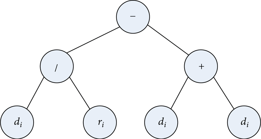
Example of a formula tree.

5. Scatter Programming Framework

In this study, SP was utilized as a methodology to generate dispatching rules. SP employs different strategies to maintain balance between intensification and diversification. The pseudocode of SP is as in Pseudocode 1.

Pseudocode 1

Step 1. Initialize Ini-Set and Ref-Set.

Step 2. Use Sub-Set generation method to initialize Sub-Set from Ref-Set.

Step 3. Create new individual solutions by Children Generation Method.

Step 4. Improve all generated solutions.

Step 5. Update Ref-Set according to the improved solutions. If the stop condition is not satisfied, go to Step 2.

5.1. Generation Method for the Initial and Reference Sets

The solutions in the initial set (Ini-Set) are generated randomly for diversification. After Ini-Set is constructed, two types of solutions are removed from Ini-Set and incorporated into Ref-Set. First, the solutions with ideal fitness are selected. Second, the distance between the remaining solutions in Ini-Set and those in Ref-Set is computed by tree edit distance (TED) [12]. For two trees t₁ and t₂, TED is the number of editions to t₁ if t₁ is modified to be equal to t₂. The distance between a solution and a solution set is defined as the sum of the distances between this solution and all solutions in this solution set. The solution whose distance to the current Ref-Set is longer than that of the other solutions in the Ini-Set is selected and added to Ref-Set. If the distance between two trees equals 0, the two trees are similar. If a selected solution in Ini-Set is similar to some solutions in Ref-Set, it will not be incorporated into Ref-Set.

5.2. Sub-Set and Children Generation Methods

In this study, all pairs of solutions in Ref-Set were selected as “parents” to generate “children” and added to Sub-Set. Children were generated from parents by one-point crossover. In the process of one-point crossover, a crossover point is selected in each parent tree. Two subtrees in parent trees are then swapped, and two children trees are constructed. Figure 2 shows an example of one-point crossover. All generated children are improved before Ref-Set updating.

Figure 2:

Example of one-point crossover.

5.3. Local Improvement Method

All solutions in Sub-Set are improved by the local improvement method. An intensification search procedure called shaking search was developed in [7]. In shaking search, n nodes in the tree are selected randomly and updated by different random alternatives. Hence, shaking search operates as a stochastic search approach. We propose one-point traversal shaking search as a local improvement method in SP to improve the intensification of shaking search. To maintain the main parts of the tree structure, we only select one node and replace it with alternatives. The best generated solution is applied to update Ref-Set. The pseudocode of the local improvement method is as in Pseudocode 2.

Pseudocode 2

Step 1. Set solution tree to ST and initialize terminal candidate set TS with five parameters

and function candidate set FS with six mathematical operators;

Step 2. Select one position p randomly in ST;

Step 3. If node n in position p belongs to the terminal set

Select one candidate parameter t from TS;

Delete t from TS;

While n ≠t

Replace note n in position p by t to generate a new solution S^′;

If the fitness value of S^′ is better than that of S,

S = S^′;

Else

Recover note t in position p by n;

While TS ≠∅;

Else

Select one candidate mathematical operator f from FS;

Delete f from FS;

While n ≠f

Replace node n in position p by f to generate a new solution S^′;

If the fitness value of S^′ is better than that of S,

S = S^′;

Else

Recover the note f in position p by n;

While FS ≠∅.

5.4. Reference Set Updating Method

The main issue in the Ref-Set updating procedure is the duplication test. In the proposed algorithm, if the TDE between two solutions is equal to 0, the two solutions are similar. When all children are improved, they are set to update Ref-Set. If the size of Ref-Set is n, then the size of Sub-Set is n(n − 1)/2. The number of children generated by Sub-Set is also n(n − 1)/2. Hence, the number of children ready for updating is larger than the size of Ref-Set when n is larger than 3. All children are selected to update Ref-Set. If a child is better than the worst solution in Ref-Set, it replaces the worst one. If a child is similar to some solutions in Ref-Set or is worse than all solutions in Ref-Set, it is dropped. The solution in Ini-Set, which is the farthest to Ref-Set, is selected to replace the worst one in Ref-Set.

6. Performance Evaluation

6.1. Parameters and Simulation Environment

The initial population size is 100, and the number of generations is 100 for both GP and SP. The crossover probability of GP is 100%. The size of the Ref-Set of SP is eight. The number of machines is five. Experiments were performed on a computer with Intel Pentium Dual E2160, 1.80 GHz, 1.79 GHz, 2 GB RAM, and Microsoft Windows XP OS.

6.2. Instance Generation

As shown in Table 1, 10 cases of the HFS problem were generated as benchmark instances. The numbers of jobs are [20, 40, 60, 100, 200], and the numbers of stages are [5, 10]. All data in each case, such as release time, process time, and due date for each job, were produced randomly. The weights of all jobs are similar.

Table 1:

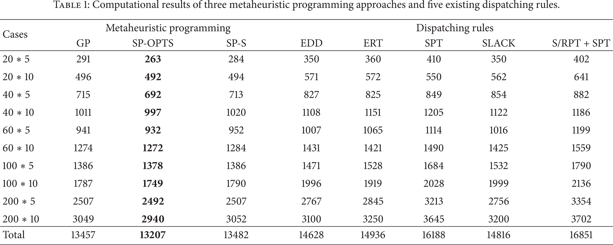
Computational results of three metaheuristic programming approaches and five existing dispatching rules.

Cases	Metaheuristic programming			Dispatching rules
Cases	GP	SP-OPTS	SP-S	EDD	ERT	SPT	SLACK	S/RPT + SPT

20*5	291	263	284	350	360	410	350	402
20*10	496	492	494	571	572	550	562	641
40*5	715	692	713	827	825	849	854	882
40*10	1011	997	1020	1108	1151	1205	1122	1186
60*5	941	932	952	1007	1065	1114	1016	1199
60*10	1274	1272	1284	1431	1421	1490	1425	1559
100*5	1386	1378	1386	1471	1528	1684	1532	1790
100*10	1787	1749	1790	1996	1919	2028	1999	2136
200*5	2507	2492	2507	2767	2845	3213	2756	3354
200*10	3049	2940	3052	3100	3250	3645	3200	3702

Total	13457	13207	13482	14628	14936	16188	14816	16851

6.3. Computational Results of Cases

The results of three metaheuristic programming approaches and five dispatching rules for 10 cases of the HFS problem are presented in Table 1. The three metaheuristic programming approaches are GP, SP with shaking [7] (SP-S), and the proposed SP with one-point traversal shaking (SP-OPTS). The five existing dispatching rules are as follows:

earliest due date (EDD): the job with the earliest due date is selected via the formula min ⁡ (d_i);

earliest release time (ERT): the job with the earliest release time is selected via the formula min ⁡ (r_i);

shortest processing time (SPT): the job with the shortest processing time on the current stage is selected via the formula min ⁡ (p_is);

SLACK (the difference between the due date and the completion time of the job with no delay): the job with minimum SLACK time is selected via the formula min ⁡ (d_i − T − w_i);

S/RPT + SPT (combination of SLACK per remaining work rule and the shortest processing time first rule): find a larger value from two computed values; one is slack time per remaining work ratio multiplied by process time in the current stage, and the other is process time in the current stage. The job with minimum value is selected. The formula is min(max(SLACK_i/w_i, p_is).

The results in Table 1 demonstrate that metaheuristic programming methods yield better solutions than existing dispatching rules in the 10 cases. The performance of GP and SP-S is similar. The results of GP are better than those of SP-S in cases 40*10, 60*5, 60*10, 100*10, and 200*10. Meanwhile, the results of GP are worse than those of SP-S in cases 20*5, 20*10, and 40*5. The results of GP and SP-S are similar in cases 100*5 and 200*5. In existing dispatching rules, the total makespan of EDD is minimum. The overall performance of S/RPT + SPT is the worst, although S/RPT + SPT yield better results than SPT in cases 20*5 and 40*10. SP-OPTS outperforms the other two metaheuristic programming approaches in all cases. The dispatching rules generated by SP-OPTS produced results better than those of existing dispatching rules in the 10 cases.

The 10 dispatching rules generated by SP-OPTS for 10 cases are described in Pseudocode 3.

Pseudocode 3

DP0:

(max ⁡ (w_i, (min ⁡ (d_i, p_is))))/((p_is + min ⁡ (w_i, p_is))/max ⁡ (w_i, T)/min ⁡ (d_i, d_i));

DP1:

(r_i + p_is)/(min ⁡ (T/w_i, r_i))*(T − w_i);

DP2:

(max ⁡ (r_i, min ⁡ (max ⁡ (T/T, w_i/r_i), d_i)))/(p_is/d_i);

DP3:

(min ⁡ ((T − p_is), (T/d_i + max ⁡ ((p_is/r_i + p_is), w_i))))*(d_i − w_i);

DP4:

p_is/w_i + min ⁡ ((d_i/min ⁡ (p_is, d_i)), min ⁡ (w_i, T));

DP5:

((w_i − p_is)/(T − p_is) − min ⁡ (T, p_is))/(w_i + r_i);

DP6:

min ⁡ ((w_i*w_i − w_i)/(d_i + p_is), (d_i/p_is));

DP7:

(w_i − p_is)/(T + max ⁡ (T, d_i) + min ⁡ (d_i, w_i));

DP8:

max ⁡ (T/p_is*w_i + ((d_i − p_is) − (T − r_i)), w_i) − p_is/r_i;

DP9:

max ⁡ (max ⁡ ((d_i*w_i), min ⁡ (T, min ⁡ (T, p_is))), (max ⁡ (d_i, T) + min ⁡ (p_is, T))).

In these 10 dispatching rules, some special subexpressions in the formulae may be obtained. For example, one part in the formula of DP0 is min ⁡ (d_i, d_i). In fact, the subexpression min ⁡ (d_i, d_i) is equivalent to d_i. These special subexpressions occupy additional branches and nodes in trees and make the formula complicated but cannot improve the results of the formula. Further work is necessary to prevent this type of expression from being constructed by SP.

The ten dispatching rules (DP0–DP9) shown in Table 1 are applied in Table 2 to solve 10 new cases. The new cases are generated in the same procedure as those described in Table 1. The dispatching rules generated by SP-OPTS produced the best results. DR0, DR1, DR4, and DR7 produced two best results in the 10 cases. DR3 and DR9 produced one best result in the 10 cases. In some cases, the results produced by the generated dispatching rules are not as good as those generated by existing dispatching rules. For example, in the case 20*5, the makespan obtained by SPT is lower than that obtained by DR9.

Table 2:

Automatically generated dispatching rules reused in other instances.

Cases	Newly generated dispatching rules										Existing dispatching rules
Cases	DR0	DR1	DR2	DR3	DR4	DR5	DR6	DR7	DR8	DR9	EDD	ERT	SPT	SLACK	S/RPT + SPT

20*5	329	363	364	356	351	355	325	323	356	336	369	389	400	377	435
20*10	496	491	503	487	475	490	501	509	518	530	540	568	519	544	519
40*5	737	788	778	763	752	745	753	744	758	776	870	784	888	822	898
40*10	1133	1117	1142	1150	1115	1168	1151	1189	1152	1108	1138	1151	1203	1154	1198
60*5	978	1003	959	1006	932	1006	958	945	1020	988	1006	1072	1209	1018	1182
60*10	1342	1377	1362	1331	1357	1349	1348	1333	1347	1380	1373	1347	1510	1413	1481
100*5	1571	1502	1570	1548	1508	1562	1587	1579	1565	1590	1571	1572	1835	1611	1822
100*10	1805	1763	1864	1778	1835	1778	1774	1781	1802	1815	1848	1906	2014	1900	2044
200*5	2552	2594	2555	2551	2553	2644	2557	2507	2639	2558	2681	2760	3231	2861	3203
200*10	2966	3005	3020	2999	3033	3025	2968	3102	2993	3041	3145	3114	3674	3174	3620

The total makespan obtained by all dispatching rules (Table 2) in the 10 cases is shown in Figure 3. The results in blue are those obtained by the generated dispatching rules and those in red are obtained by existing dispatching rules. The total makespan obtained by DP0–DP9 is obviously smaller than that of existing dispatching rules. Hence, the dispatching rules generated automatically by SP-OPTS can be potentially reused in the new problem instance.

Figure 3:

Total makespan obtained by the different dispatching rules in Table 2.

Five parameters in the terminal set appear in the 10 generated formulae of dispatching rules. Parameters p_is and w_i are present in all 10 generated dispatching rules (Table 3). They play an important role in the generation of dispatching rules. Parameters d_i and T are present in eight and nine dispatching rules, respectively. In the 10 generated dispatching rules, parameter r_i occurs significantly less often than the other parameters. It only appears in five dispatching rules. The results of these five dispatching rules are not as good as those of other dispatching rules, such as DR0, DR4, and DR6. Hence, parameter r_i is not as important as other parameters for constructing dispatching rules to schedule candidate jobs. We believe the reason is that all candidate jobs ready for scheduling have been released. Jobs that have not been released will not be assigned a priority score by the dispatching rules.

Table 3:

Parameters present in the generated dispatching rules.

Parameters	Generated dispatching rules

r _i	DP1, DP2, DP3, DP5, DP8
p _is	DP0, DP1, DP2, DP3, DP4, DP5, DP6, DP7, DP8, DP9
d _i	DP0, DP2, DP3, DP4, DP6, DP7, DP8, DP9
w _i	DP0, DP1, DP2, DP3, DP4, DP5, DP6, DP7, DP8, DP9
T	DP0, DP1, DP2, DP3, DP4, DP5, DP7, DP8, DP9

The convergence rate of the two SPs (SP-S and SP-OPTS) in three cases (60*5, 100*5, and 200*5) is shown in Figure 4. The x-axis represents the number of iterations. The numbers on the y-axis are makespan values. In the case 60*5, SP-OPTS converges after 20 iterations. In cases 100*5 and 200*5, SP-OPTS converges after five iterations. SP-OPTS achieves faster convergence rates than SP-S in three cases. The makespan generated by SP-OPTS is smaller than that generated by SP-S.

Figure 4:

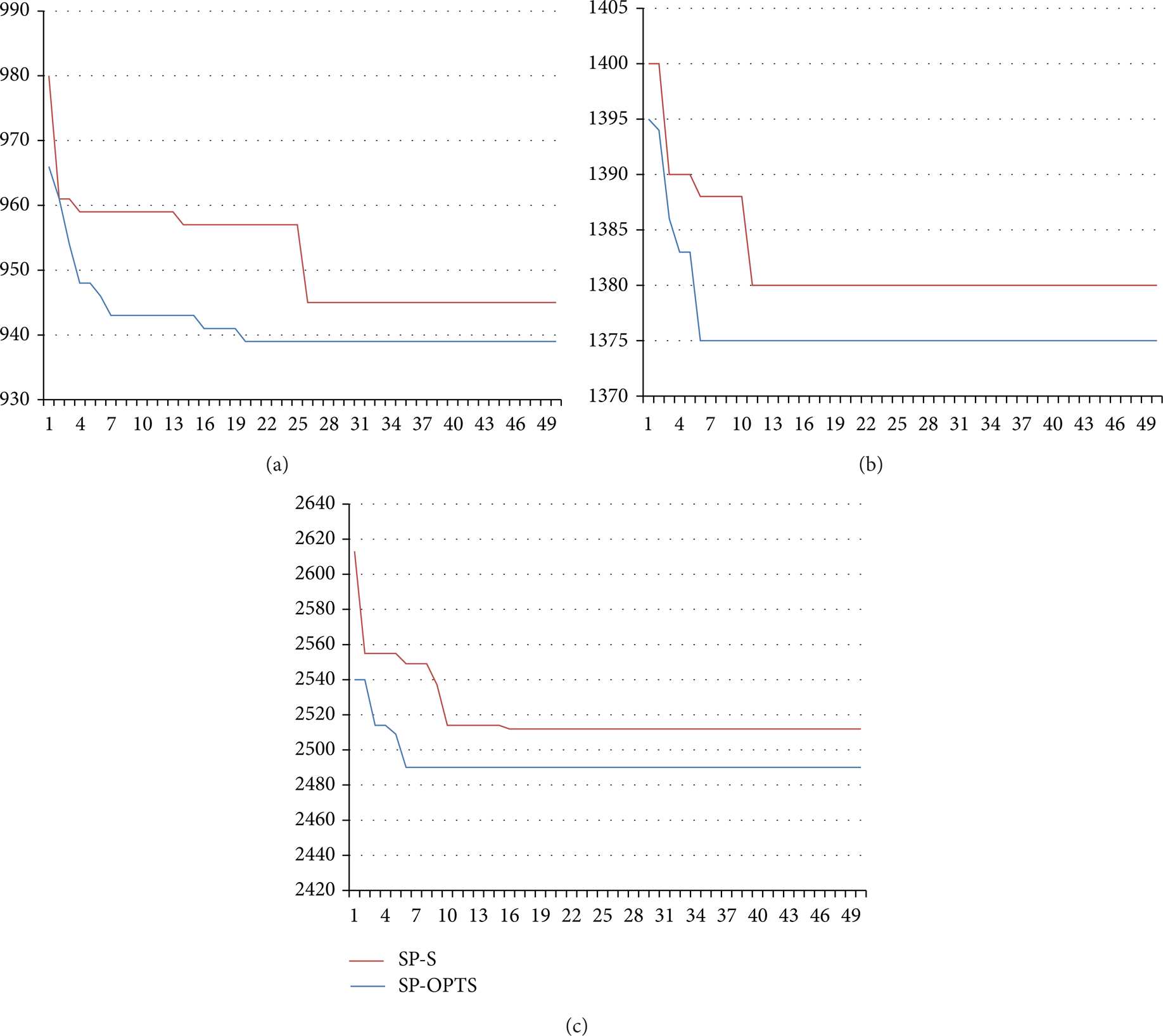
(a) Comparison of the convergence rate in the case 60*5. (b) Comparison of the convergence rate in the case 100*5. (c) Comparison of the convergence rate in the case 200*5.

7. Conclusions and Future Work

Dispatching rules are widely used to solve the HFS problem. In this study, an SP approach was developed to generate new dispatching rules automatically for each instance of the problem. Our proposed SP approach includes an enhanced local improvement method, namely, one-point traversal shaking. The simulation results show that our proposed algorithm outperforms other metaheuristic programming methods, such as GP and SP-S. The dispatching rules generated by our approach not only yield better results but also have the potential to be reused in new cases. The one-point traversal shaking search proposed in this paper is a local improvement method that can improve the rate of convergence.

In the future, reinforcement learning should be applied to the local improvement method in SP. Different machines at different stages play different roles in HFS. Hence, an enhanced SP for automatically generating different dispatching rules for each machine is required.

Conflict of Interests

The authors declare that there is no conflict of interests regarding the publication of this paper.

Footnotes

Acknowledgments

This study is supported by grants from the National Natural Science Foundation of China and Civil Aviation University of China (61039001) and Tianjin Municipal Science and Technology Commission (11ZCKFGX04200).

References

Gupta

J. N. D.

, “Two-stage, hybrid flowshop scheduling problem,” Journal of the Operational Research Society, vol. 39, no. 4, pp. 359–364, 1988.

Lee

G.-C.

and Kim

Y.-D.

, “A branch-and-bound algorithm for a two-stage hybrid flowshop scheduling problem minimizing total tardiness,” International Journal of Production Research, vol. 42, no. 22, pp. 4731–4743, 2004.

Wang

and Tang

, “A tabu search heuristic for the hybrid flowshop scheduling with finite intermediate buffers,” Computers and Operations Research, vol. 36, no. 3, pp. 907–918, 2009.

Naderi

Zandieh

, and Roshanaei

, “Scheduling hybrid flowshops with sequence dependent setup times to minimize makespan and maximum tardiness,” International Journal of Advanced Manufacturing Technology, vol. 41, no. 11–12, pp. 1186–1198, 2009.

Liu

, and Wu

, “A genetic algorithm for solving flow shop scheduling problems with parallel machine and special procedure constraints,” in Proceedings of the International Conference on Machine Learning and Cybernetics, pp. 1774–1779, IEEE, November 2003.

Koza

J. R.

, Genetic Programming: On the Programming of Computers by Means of Natural Selection, vol. 1, MIT Press, 1992.

Hedar

A.-R.

and Osman

M. K.

, “Scatter programming,” in Proceedings of the 2nd International Conference on Computer Technology and Development (ICCTD '10), pp. 451–455, IEEE, November 2010.

Dimopoulos

and Zalzala

A. M. S.

, “Investigating the use of genetic programming for a classic one-machine scheduling problem,” Advances in Engineering Software, vol. 32, no.6, pp. 489–498, 2001.

Geiger

C. D.

Uzsoy

, and Aytuğ

, “Rapid modeling and discovery of priority dispatching rules: an autonomous learning approach,” Journal of Scheduling, vol. 9, no. 1, pp. 7–34, 2006.

10.

Jakobović

Jelenković

, and Budin

, “Genetic programming heuristics for multiple machine scheduling,” in Genetic Programming, vol. 4445 of Lecture Notes in Computer Science, pp. 321–330, Springer, Berlin, Germany, 2007.

11.

Tay

J. C.

and Ho

N. B.

, “Evolving dispatching rules using genetic programming for solving multi-objective flexible job-shop problems,” Computers and Industrial Engineering, vol. 54, no. 3, pp. 453–473, 2008.

12.

Laguna

Marti

, and Martí

R. C.

, Scatter Search: Methodology and Implementations in C, vol. 24, Springer, Berlin, Germany, 2003.

13.

Ochoa

Vázquez-Rodríguez

J. A.

Petrovic

, and Burke

, “Dispatching rules for production scheduling: a hyper-heuristic landscape analysis,” in Proceedings of the IEEE Congress on Evolutionary Computation (CEC '09), pp. 1873–1880, IEEE, May 2009.

14.

Brah

S. A.

, “A comparative analysis of due date based job sequencing rules in a flow shop with multiple processors,” Production Planning and Control, vol. 7, no. 4, pp. 362–373, 1996.

Automatic Heuristic Generation with Scatter Programming to Solve the Hybrid Flow Shop Problem

Abstract

1. Introduction

2. Formulation of the HFS Problem

3. Related Work

3.1. Dispatching Rules for HFS

3.2. GP

3.3. SP

4. Solution Representation

4.1. Terminal Set

4.2. Function Set

5. Scatter Programming Framework

Pseudocode 1

5.1. Generation Method for the Initial and Reference Sets

5.2. Sub-Set and Children Generation Methods

5.3. Local Improvement Method

Pseudocode 2

5.4. Reference Set Updating Method

6. Performance Evaluation

6.1. Parameters and Simulation Environment

6.2. Instance Generation

6.3. Computational Results of Cases

Pseudocode 3

7. Conclusions and Future Work

Conflict of Interests

Footnotes

Acknowledgments

References