Energy-Efficient Node Selection Algorithms with Correlation Optimization in Wireless Sensor Networks

Abstract

The sensing data of nodes is generally correlated in dense wireless sensor networks, and the active node selection problem aims at selecting a minimum number of nodes to provide required data services within error threshold so as to efficiently extend the network lifetime. In this paper, we firstly propose a new Cover Sets Balance (CSB) algorithm to choose a set of active nodes with the partially ordered tuple (data coverage range, residual energy). Then, we introduce a new Correlated Node Set Computing (CNSC) algorithm to find the correlated node set for a given node. Finally, we propose a High Residual Energy First (HREF) node selection algorithm to further reduce the number of active nodes. Extensive experiments demonstrate that HREF significantly reduces the number of active nodes, and CSB and HREF effectively increase the lifetime of wireless sensor networks compared with related works.

1. Introduction

A wireless sensor network consists of spatially sensor nodes which are generally self-organized and connected by wireless communications [1]. Today such networks are used in many industrial and consumer applications, such as traffic data collection, vehicular monitoring and control, security surveillance, and smart homes. Each sensor node is equipped with a sensing device which can detect the environmental condition. The nodes are also powered by limited batteries and it is difficult or impossible to replace them in some special environments. It is why energy efficiency is always the most important criterion for such networks. One important approach to extend the network lifetime is to reduce the number of required packet transmissions in the network [2–5], such as clustering [6–11], in-network data aggregation [12–18], and approximate data collection [19, 20]. In these scenarios, all nodes in the network are considered active and the data are gathered from all nodes during the collecting process.

However, it is not an efficient way to collect all raw data from each node in some special applications which aim to collect information originated from the environment, such as temperature, humidity, and pressure. In these applications, it is fully tolerant if the final collected information is just within error threshold. The sensing data of each node is generally a noise version of the observed phenomenon and there is a deviation among them due to distance, location, or node sensitivity. Nodes are generally correlated if they are observing the same physical phenomena. Correlations between nodes are described in some simple ways such as the maximum or minimum value between nodes [21]. In this paper, correlation occurs if the sensing data of simple node can be obtained from the other nodes. Accordingly, a subset of active nodes can be selected to provide the required sensing service within error threshold, and the rest nodes can go to sleep and preserve energy. In this way, the active node selection strategy with correlation optimization not only prolongs the network lifetime, but also helps to solve other issues in dense wireless sensor networks [22], such as lower network throughput, serious node conflict, and excessive packet transmissions.

How to describe the correlation among the sensing data quantitatively is the key issue when achieving an efficient active node selection strategy. The distance function is generally considered as an important model to formulate the data similarity between nodes because the sensitivity is sometime related to the distance between the source and sensing device. Here we adopt Manhattan distance between sensing data as error metric [22]. Based on the observation that the sensing data are similar to each other if they are close enough, Kotidis [23] proposes Snapshot query in which only selected active nodes report their sensing data, and sensing data of one-hop nodes is computed by active nodes. Liu et al. [24] propose an EEDC algorithm which divides the nodes into disjoint cliques based on spatial correlation so that the nodes in the same clique have similar sensing data and can communicate directly with each other. Hung et al. [22] propose a DCglobal algorithm to determine a set of active nodes with high energy levels and wide data coverage ranges.

Figures 1(a) and 1(b) show the selected nodes with EEDC and DCglobal for a given wireless sensor network, where each circle denotes one node (the sensing data value is marked above the circle). The edge between a pair of nodes denotes that they can communicate directly with each other. Here we assume that Manhattan distance is used as the similarity function and the error threshold is 0.5. The selected active nodes are marked with black solid circle. The selected active node set with EEDC is $\{s_1,s_2,s_5,s_6,s_8,s_9,s_{12}\}$ , and it is $\{s_1,s_5,s_{10},s_{13}\}$ with DCglobal. According to Figure 1, the number of selected nodes with DCglobal is smaller than EEDC in this example.

Figure 1

An example to demonstrate different algorithms. (a) EEDC, (b) DCglobal, (c) CSB, and (d) HREF.

The concept of data coverage range is firstly introduced to describe the correlation among nodes and defined as a node set in which the distance between each element and the given node is within the error threshold [22]. In fact, it is a simple extension of one-hop data coverage [23]. Another issue of [22] is the efficiency of proposed node selection algorithm. The partially ordered tuple (residual energy, data coverage range) is used to select an active node set, which ensures that the selected nodes always have high reserved energy, but the number of selected active nodes is not minimized.

To address these problems, we introduce several new concepts, that is, cover set, active node, and covered node, and propose a new Cover Sets Balance algorithm (CSB) to choose a set of active nodes with wide data coverage range and high energy level by using the partially ordered tuple (data coverage range, residual energy) and build the corresponding cover set in sequence to ensure the selected active nodes have high residual energy. In this way, the set of final selection nodes generally owns larger residual energy and smaller size, which helps to extend the network lifetime. Figure 1(b) demonstrates the set $\{s_1,s_5,s_{10},s_{13}\}$ generated by DCglobal assuming that reserved energy is identical to all nodes in the network, which is similar to the partially ordered tuple (data coverage range, residual energy). Figure 1(c) demonstrates the result as $\{s_3,s_5,s_{10},s_{13}\}$ with the proposed CSB algorithm in this paper. $\{s_1,s_7,s_8\}$ is a cover set for node $s_3$ and each node in the set is a feasible candidate regarding $s_3$ .

In the following we show some nodes can be further removed from the selected active node set with CSB. As shown in Figure 1(c), the sensing data of $s_3$ , $s_5$ , $s_{10}$ is 35.5, 36.1, and 34.5, respectively, the average value of $s_5$ and $s_{10}$ is 35.3. The Manhattan distances between 35.3 and sensing data $s_1$ , $s_3$ , $s_7$ , and $s_8$ are 0.1, 0.2, 0.1, and 0.3 accordingly (they are all less than the error threshold 0.5). It means that the sensing data of ${\text{CS}}_3+\{s_3\}$ is computed by $s_5$ and $s_{10}$ . Accordingly, $s_3$ is removed and then we have a smaller active node set $\{s_5,s_{10},s_{13}\}$ , as shown in Figure 1(d). Following this observation, we introduce a novel concept Correlated Node Set (CNS) and then we propose a High Residual Energy First (HREF) node selection algorithm to reduce the number of active nodes. The main contributions of this paper are as follows.

• (i)

We propose a Cover Sets Balance algorithm (CSB) to select a set of active nodes with wide data coverage ranges and high energy levels. In each active node selection step, we use the partially ordered tuple (data coverage range, residual energy) to find an initial active node set and then balance the size of the cover sets in order to replace low-energy nodes.

(ii)

We propose a Correlated Node Set Computing algorithm (CNSC) to calculate the correlated node set with minimum set size and maximum geometric mean of residual energy of each node in the sensor network by following the observation that some nodes selected by CSB can be further removed.

(iii)

We propose a High Residual Energy First algorithm (HREF) to reduce the number of active nodes selected with CSB by removing nodes which can be computed by correlated node sets.

The rest of this paper is organized as follows. In Section 2, we describe the system model. Section 3 introduces CSB and HREF algorithms. The theoretical analysis of the algorithms is proposed in Section 4. In Section 5, we describe the simulation results and performance analysis. Section 6 presents the related works and Section 7 is conclusion.

2. System Model

A wireless sensor network generally consists of a set of stationary nodes $V=\{s_1,s_2,\dots ,s_n\}$ , and each node in the network has identical transmission radius r. The network is formulated as an undirected graph $G=(V,E)$ with V as the set of nodes and E as the set of links. Without loss of generality, both $s_i$ and i are used to represent one single node in the network. There is a link $(i,j)$ between node i and j if they communicate with each other directly.

The nodes are equipped with unreplaceable or unrechargeable batteries. The reserved energy for node i at time t is denoted by $e_i(t)$ . The collected data from one single node is a noise version of the practical phenomena. In these applications, the collected information from the sensor network is tolerant in case that it is within a given error threshold ɛ.

The notations used in this work are listed as the following:

•  

$V\text{:}$ Set of nodes in the network

  

n: Number of nodes in the network

  

ε: One given error threshold

  

$x_i(t)$ : Sensing data of i at time t

  

$d(x_i(t),x_j(t))$ : Distance between the sensing data of i and j

  

${\text{Energy}}_i(t)$ : Residual energy of i at time t

  

${\text{DCR}}_i$ : Data coverage range of i

  

${\text{CS}}_i$ : Cover set of i

  

${\text{CNS}}_i$ : Correlated node set of i

  

$\text{ANS}$ : Active node set

  

r: Transmission radius

  

$maxd$ : Maximal number of nodes in a correlated node set

  

${\text{Event}}_j(t)$ : Value of event j at time t

  

Interval: Interval to reselect a new active node set.

The correlation among sensing data especially in a dense wireless sensor network is helpful to extend the network lifetime. Some researchers studied the correlation between nodes and provided some models [25]. Among all these models, it is common to adopt distance function, such as Manhattan distance $d(x_i(t),x_j(t))$ to represent the correlation between sensing data $x_i(t)$ and $x_j(t)$ at time t [22], which is represented as $d(x_i(t),x_j(t))=|x_i(t)-x_j(t)|$ . Without loss of generality, we follow this correlation model in this paper. Note that our algorithms are adapted to any other correlation models with minor modification.

The sensing data of $s_j$ is called to be computed with the sensing data of $s_i$ if the sensing data has a high correlation level; that is, $d(x_i(t),x_j(t))\le \epsilon$ , where ɛ is the given error threshold. $S_j$ is also in the data coverage range of $s_i$ . The definitions are given as follows.

Definition 1 (data coverage range (DCR)).

Given an error threshold ε in the sensor network, the data coverage range ${\text{DCR}}_i$ of i is a subset of V, in which Manhattan distance from each node to i is no more than ε, and $i\notin {\text{DCR}}_i$ .

For the example in Figure 1(b), $\epsilon =0.5$ , ${\text{DCR}}_1=\{s_3,s_6,s_7,s_8\}$ , ${\text{DCR}}_3=\{s_1,s_4,s_7,s_8\}$ , and so on.

Definition 2 (active node set (ANS) and active node).

Given a sensor network $G=(V,E)$ , an active node set (ANS) is a subset of V, in which each $i\in V$ either belongs to ANS or one data coverage range ${\text{DCR}}_j$ , where $j\in \text{ANS}$ . Any node in ANS is named as an active node.

For the example in Figure 1(c), $\text{ANS}=\{s_3,s_5,s_{10},s_{13}\}$ and each node in the set is an active node.

Definition 3 (cover set (CS) and covered node).

Given a sensor network $G=(V,E)$ and according ANS, the cover set ${\text{CS}}_i$ for any given $i\in \text{ANS}$ is a subset of ${\text{DCR}}_i$ , and ${\text{CS}}_i\cap {\text{CS}}_j=\varnothing$ in case $i\ne j$ . Any node in ${\text{CS}}_i$ is named as a covered node.

For the example in Figure 1(c), ${\text{CS}}_3=\{s_1,s_7,s_8\}$ , $s_3$ is the active node, and $s_1$ , $s_7$ , and $s_8$ are covered nodes.

Sensor data is affected by the events in monitored region, and the influence of each event on a sensor is inversely proportional to their distance. Here we assume that correlation occurs among all active nodes in the sensor network.

Definition 4 (correlated node set ( $\text{CNS}$ )).

Given a sensor network $G=(V,E)$ and its corresponding $\text{ANS}$ , the correlated node set ${\text{CNS}}_i$ for $i\in \text{ANS}$ is a subset of $\text{ANS}$ , and the arithmetic mean $\stackrel{-}{s}$ for sensing data of nodes in ${\text{CNS}}_i$ satisfies the error threshold condition; that is, $d(x_j(t),\stackrel{-}{s})\le \epsilon$ , $j\in {\text{CS}}_i+\{i\}$ . The sensing data of ${\text{CS}}_i+\{i\}$ is said to be computed by ${\text{CNS}}_i$ .

For the example in Figure 1(d), ${\text{CNS}}_3=\{s_5,s_{10}\}$ , $\stackrel{-}{s}=35.3$ , $d(x_1,\stackrel{-}{s})=0.2\le \epsilon$ , $d(x_7,\stackrel{-}{s})=0.1\le \epsilon$ , $d(x_8,\stackrel{-}{s})=0.3\le \epsilon$ , $d(x_3,\stackrel{-}{s})=0.2\le \epsilon$ .

Definition 5 (CNS computing problem).

Given a sensor network $G=(V,E)$ , ANS, sensing data $X=\{x_1,x_2,\dots ,x_n)$ , cover sets $\text{CS}=({\text{CS}}_{\mathrm{1}},{\text{CS}}_{\mathrm{2}},\dots ,{\text{CS}}_n)$ , and reserved energy $\text{Energy}=\{e_1,e_2,\dots ,e_n\}$ , the CNS computing problem is to find a correlated node set ${\text{CNS}}_i$ for node $i\in \text{ANS}$ , and the size of $\left|{\text{CNS}}_i\right|$ is minimized while the geometric mean of residual energy $\widehat{e}$ is maximized, where $\widehat{e}=\sqrt[n]{e_{\mathrm{1}}{e}_{\mathrm{2}}\cdots e_n}$ .

Note that we adopt the geometric average of the residual energy in the correlated node set by following the observation that the average geometric averaging gives higher results for lower variations in the data values for a given data set with a fixed arithmetic [26].

Definition 6 (active node selection problem).

Given a sensor network $G=(V,E)$ , the sensing data $X=\{x_1(t),x_2(t),\dots ,x_n(t)\}$ , reserved energy levels $\text{Energy}(t)=\{e_1(t),e_2(t),\dots ,e_n(t)\}$ at time t and given threshold ɛ, the active node selection problem is to select a set of active nodes $\text{ANS}(t)$ at time t, where all sensing data in the network can be computed by their corresponding active nodes, and the network lifetime is maximized, that is, $\max \{t\}$ .

The active node selection problem is to find the active node set during each epoch and aim at maximizing the network lifetime. The problem is proven to be NP-hard by mapping it to the set covering problem or minimum dominating set problem [26–28]. In this paper, we design two heuristic algorithms, namely, CSB and HREF for this problem.

3. Heuristic Algorithms

3.1. CSB Algorithm

Most related works use the concept of data coverage range combined with energy to solve the active node selection problem. In this section we illustrate the Cover Sets Balance algorithm (CSB) based on the idea of data coverage range.

In data collection process, only active nodes are required to provide perception service, and the rest nodes are closed to preserve energy. An intuitive approach for the node selection process is to use the partially ordered tuple (data coverage range, residual energy) [23]. Another approach is to use partially ordered tuple (residual energy, data coverage range) to select active nodes with higher residual energy [22]. However, the number of selected nodes is generally larger than the former approach, which means that more energy consumption is necessary when providing perception service during the given epoch. Obviously, we need a balance between the two metrics, that is, the data coverage range and residual energy.

The basic idea of Cover Sets Balance (CSB) algorithm is described as the following: (1) generate an initial active node set and the corresponding cover sets through the previous data coverage range priority strategy; (2) replace active nodes with high-energy candidates. Note that the candidates must cover all nodes within the same cover set. For example, in Figure 1(b), ${\text{CS}}_1=\{s_3,s_6,s_7,s_8\}$ , $\text{C}{\text{S}}_{\mathrm{5}}=\{s_2,s_4\}$ , ${\text{CS}}_{10}=\{s_{11}\}$ , and ${\text{CS}}_{13}=\{s_9,s_{12}\}$ . It is seen that $s_1$ covers four nodes, namely, $s_3,\hspace{0.17em}{s}_6,\hspace{0.17em}{s}_7$ , and $s_8$ , and thus the candidate node for $s_1$ must cover the above four nodes too. However, if the cover set is too large, it is possible to find no candidate nodes. The case is similar when the cover set is too small. Obviously we need a new method to provide more candidate nodes so that the network lifetime is extended in an efficient way.

We adopt a cover set balance strategy to balance the set size by moving nodes from larger cover sets to smaller ones. The initial cover sets are sequenced in descending order of the set size, and then we check nodes in one cover set and try to move them to another with smaller size. This process continues until all sets are checked and finally they are balanced. This strategy is helpful to increase the number of candidate nodes with higher residual energy by cutting down the maximal deviation of each cover set in the balance progress.

The final step of the CSB algorithm is to replace the selected active nodes with candidates by order of reserved energy. In this way, we finally build an active node set with the same size as its initial version but higher residual energy, which is helpful to extend the network lifetime.

The CSB algorithm can be divided into three processes and pseudocodes are shown in Algorithm 1.

Algorithm 1: Pseudocodes for Cover Set Balance (CSB) algorithm.

Input: G = (V, E), ɛ , X = $\{x_1,x_2,\dots ,x_n\}$ , Energy = $\{e_1,e_2,\dots ,e_n\}$ ;

Output: ANS, CS.

(1) //Initialization_Process ( )

(2) Calculate DCR = {DCR₁, DCR₂, …, ${\text{DCR}}_n\}$

(3) Set the state of all nodes as Un-Covered;

(4) Sort nodes into sequence with partially ordered tuple $〈\text{data coverage range, residual energy}〉$ ;

(5) ANS ←∅, CS ←∅;

(6) for one maximal i in the sequnce with state as Un-Covered

(7)  ANS ← $\{i\}$ + ANS, and set i as Primary-Covered;

(8)  for each j∈ ${\text{DCR}}_i$   − ANS with state as Un-Covered

(9)    ${\text{CS}}_i\leftarrow \{j\}+{\text{CS}}_i$ , and set j as Primary-Covered;

(10)  end  for

(11) end  for

(12) //Cover_Set_Balance_Process ( )

(13) Sort CS into a sequence with decreasing order of the set size;

(14) for each ${\text{CS}}_i$ in the sequence

(15)  Sort nodes in ${\text{CS}}_i$ with decreasing order of their deviation to i;

(16)  for each j in the sequence

(17)   find out all k which satisfies $j\in {\text{CS}}_k$ and $\left|{\text{CS}}_k\right|<\left|{\text{CS}}_i\right|$ , select k with minimal cover set size;

(18)    ${\text{CS}}_i\leftarrow {\text{CS}}_i-\{j\}$ , ${\text{CS}}_k\leftarrow {\text{CS}}_k+\{j\}$ ;

(19)  end  for

(20) end  for

(21) //Node_Replace_Process ( )

(22) for each $i\in \text{ANS}$

(23)  for each $j\in {\text{CS}}_i$

(24)   if $d(x_j,x_k)\le \epsilon$ for any $k\in {\text{CS}}_i+\left\{i\right\}-\{j\}$ , then mark j as a candidate of i;

(25)  end  for

(26)  select a node m from all candidates of i with maximal residual energy $e_i$ ;

(27)  ANS ← ANS + $\{m\}-\{i\}$ ; ${\text{CS}}_m={\text{CS}}_i+\{i\}-\{m\}$ ;

(28) end  for

The Initialization_Process is used to build a primary active node set and corresponding cover sets. The basic steps are described as follows. There are two different states for each node in the network, namely, Primary-Covered and Un-Covered, which are used to mark whether it is within the cover set of one node in the active node set. The states for all nodes are initialized as Un-Covered (Line 3). Then we sort nodes with partially ordered tuple (data coverage range, residual energy) and initialize the active node set as empty set (Line 4-5). Finally, we check nodes in sequence with state as Un-Covered, and add them into the active node set if the required conditions are satisfied (Line 6–11).

The Cover_Set_Balance_Process aims at balancing the size of cover sets generated with the Initialization_Process. Firstly, the cover sets are ordered and checked accordingly to their set size (Line 13). Secondarily, nodes in a given cover set ${\text{CS}}_i$ are sorted into a sequence with descending order of their deviation to i (Line 15), and they are moved to another cover set with smaller size (Line 16–19). This process continues until all nodes in the cover set are checked (Line 14–20).

The Node_Replace_Process focuses on nodes exchange by replacing the low-energy active nodes with high-residual-energy candidates. All feasible candidate nodes of i are checked (Line 23–25), and we select the one (marked as m) with maximal residual energy among all these candidates (Line 26). Finally, the active node set is updated as well as the cover set for node m (Line 27).

The CSB algorithm follows the idea of replacing the active nodes with candidates with higher residual energy. However, it has the same number of active nodes compared with the approach which only uses the partially ordered tuple (data coverage range, residual energy). In the following we introduce a new HREF algorithm to further reduce the number of active nodes based on CNSC algorithm.

3.2. HREF Algorithm

We first introduce an algorithm for the CNS computing problem and then propose a High Residual Energy First node selection algorithm (HREF) for the active node selection problem.

3.2.1. CNSC Algorithm

The CNS computing problem is to find one subset ${\text{CNS}}_i$ for $i\in \text{ANS}$ and aim at minimizing ${\text{CNS}}_i$ as well as maximizing the geometric mean of residual energy $\widehat{e}=\sqrt[n]{e_{\mathrm{1}}{e}_{\mathrm{2}}\cdots e_n}$ . To find out the optimal ${\text{CNS}}_i$ , an intuitive way is to calculate the average value of sensing data for each subset ANS stored in a sequenced list L. Then, pick out the average values whose deviation is no more than ε and the corresponding correlated node set in the list. Finally, select the ${\text{CNS}}_i$ with minimized node set and maximum geometric mean of residual energy as the final correlated node set for i. Obviously, the above solution is to find the optimal result but has exponential time complexity $(O(2^{\left|\text{ANS}\right|}))$ .

To reduce the time complexity, we assume each ${\text{CNS}}_i$ has at most $maxd$ nodes, where $maxd$ is a given value depending on the network environment. The CNS computing problem is then converted to the problem of selecting at most $maxd$ number of nodes in ANS within the error threshold. Then, calculate each subset combined with the selected $maxd$ nodes and add its average value into L with the following iteration process: in the ith iteration, the average value for each subset of $\{x_1,x_2,\dots ,x_i\}$ is calculated based on the average value of subset of $\{x_1,x_2,\dots ,x_{i-1}\}$ . There are two basic operations in the iteration process, namely, $(L+x)$ and merge $L[L,L+x]$ . $\hspace{0.17em}(L+x)$ represents the new list by adding x into each element in the initial sequence L, as shown in Form. (1); and merge $L[L,L+x]$ represents the ordered list for the combined result of L and $(L+x)$ :

$$\begin{array}{cc}& L+x=\left\{\frac{L\left(i\right)\times L\_\text{count}\left(i\right)+x}{L\_\text{count}\left(i\right)+\mathrm{1}}:i\in L\right\},\end{array}$$

(1)

where $L(i)$ denotes the ith data in L, and L_count $(i)$ denotes number of nodes from which the average value is calculated.

Here we demonstrate an example to illustrate the two basic operations. Let $L=\{\mathrm{0},\mathrm{36.1},\mathrm{34.5},\mathrm{35.3}\}$ , and $L\_\text{count}=\{\mathrm{0},\mathrm{1},\mathrm{1},\mathrm{2}\}$ . Then, $L+\mathrm{36.9}=\{(\mathrm{0}\times \mathrm{0}+\mathrm{36.9})/(\mathrm{0}+\mathrm{1})$ , $(\mathrm{36.1}\times \mathrm{1}+\mathrm{36.9})/(\mathrm{1}+\mathrm{1})$ , $(\mathrm{34.5}\times \mathrm{1}+\mathrm{36.9})/(\mathrm{1}+\mathrm{1})$ , $(\mathrm{35.3}\times \mathrm{2}+\mathrm{36.9})/(\mathrm{2}+\mathrm{1})\}=\{\mathrm{36.9},\mathrm{36.5},\mathrm{35.7},\mathrm{35.83}\}$ . And merge $L[L,L+36.9]=\{0,36.1,34.5,35.3\}+\{36.9,36.5,35.7,35.83\}=\{0,34.5,36.1,35.3,36.9,36.5,35.7,35.83\}$ , $L\_\text{count}=\{0,1,1,2\}+\{1,2,2,3\}$ $=$ $\{0,1,1,2,1,2,2,3\}$ .

In the following we illustrate the CNS computing process for $s_3$ in Figure 1(c) by assuming that the residual energy is identical to all. The input for the CNS computing problem is described as ${\text{CS}}_3=\{s_1,s_3,s_7,s_8\}$ , $\text{ANS}-\{s_3\}=\{s_5,s_{10},s_{13}\}$ , and $X=\{36.1,34.5,36.9\}$ . Initially, $L=\{0\}$ , $L\_\text{count}=\{0\}$ , and the corresponding set list as $\{\{\varnothing \}\}$ .

• (1)

Consider the sensing data 36.5 of $s_5:L=\{0,36.1\}$ , $L\_\text{count}=\{0,1\}$ , and the corresponding set list as $\{\{\varnothing \},\{s_5\}\}$ ;

(2)

consider the sensing data 34.5 of $s_{10}:L=\{0,36.1\}+\{34.5,35.3\}=\{0,36.1,34.5,35.3\}$ , $L\_\text{count}=\{0,1,1,2\}$ , and the corresponding set list as $\{\{\varnothing \},\{s_5\},\{s_{10}\},\{s_5,s_{10}\}\}$ ;

(3)

consider the sensing data 36.9 of $s_{13}:L=\{0,36.1,34.5,35.3\}$ + $\{36.9,36.5,35.7,35.83\}$ $=$ $\{0,34.5,36.1,35.3,36.9,36.5,35.7,35.83\}$ , $L\_\text{count}=\{0,1,1,2,1,2,2,3\}$ , and the set list as $\{\{\varnothing \},\{s_5\},\{s_{10}\},\{s_5,s_{10}\},\{s_{13}\}$ , $\{s_5,s_{13}\},\{s_{10},s_{13}\}$ , $\{s_5,s_{10},s_{13}\}\}$ .

The deviation between 35.3 and the sensing data of nodes in set ${\text{CS}}_3+\{s_3\}$ is no more than 0.5, and it is similar to 35.7. Accordingly, the corresponding correlated node sets are $\{s_5,s_{10}\}$ and $\{s_5,s_{10},s_{13}\}$ located at the 4th and 7th positions in L. Finally, ${\text{CNS}}_3=\{s_5,s_{10}\}$ followed by $|\{s_5,s_{10}\}|<|\{s_5,s_{10},s_{13}\}|$ .

Algorithm 2 provides the pseudocodes for CNSC algorithm.

Algorithm 2: Pseudocodes for CNSC algorithm.

Input: ANS, ɛ, CS = $\{{\text{CS}}_1,{\text{CS}}_2,\dots ,{\text{CS}}_n\}$ , $X=\{x_1,x_2,\dots ,x_n\}$ , Energy = $\{e_1,e_2,\dots ,e_n\}$ ;

Output: ANS.

(1) for each i in ANS

(2)   ${\text{CNS}}_i=\varnothing$ ;

(3)  for each maxd nodes in ANS

(4)   placed them in node_vector;

(5)    $L[0]=\{0\}$ ;

(6)   for  j = 1 to $\left|node\_vector\right|$ , L = mergeL $(L,L+x_{node\_vector(j)})$ ;

(7)   for each l in $L[i]$

(8)    for each   $k\in {\text{CS}}_i+\{i\}$ if $\left|l-x{}_k\right|\le \epsilon$   then temp = L_pos(l);

(9)    for  k = $\left|node\_vector\right|$ − 1 to 0

(10)     if  temp > $2^k$ and temp ≤ $2^{(k+1)}$

(11)      Dset = Dset + {the kth node in node_vector}, temp = temp – $2^k$ ;

(12)     end if

(13)    end for

(14)    if ( $\left|Dset\right|$ < $\left|{\text{CNS}}_i\right|$ ) or ( $\left|Dset\right|$ = $\left|{\text{CNS}}_i\right|$ and ê( $\left|Dset\right|$ ) > ê( $\left|Dset\right|$ ), then ${\text{CNS}}_i$ ←Dset;

(15)   end for

(16)  end for

(17) end for

3.2.2. HREF Algorithm

For a given $i\in \text{ANS}$ , its sensing data is computed with the nodes in ${\text{CNS}}_i$ , which makes it possible to shut off to preserve energy. The basic idea of the HREF algorithm is described as follows: (1) build the active node set ANS with CSB algorithm; (2) for each $i\in \text{ANS}$ , calculate its correlated node set ${\text{CNS}}_i$ ; (3) remove certain active nodes from ANS. The pseudocodes are shown in Algorithm 3.

Algorithm 3: Pseudocodes for HREF algorithm.

Input: G = (V, E), ɛ , $X=\{x_1,x_2,\dots ,x_n\}$ , Energy = $\{e_1,e_2,\dots ,e_n\}$ ;

Output: ANS.

(1) Run CSB algorithm to obtain the initial ANS and CS;

(2) Run CNSC algorithm to obtain CNS;

(3) Mark all nodes in ANS as Un-Completed;

(4) Sort CNS with increasing order of their set size;

(5) for one minimal ${\text{CNS}}_i$ in the sequence with ${\text{CNS}}_i\subseteq \text{ANS}$

(6)  if   ${\text{CNS}}_i\ne \varnothing$ , and the state of i is Un-Completed, then

(7)  ANS ← ANS −   $\{i\}$ ;

(8)  for each j∈ ${\text{CNS}}_i$ , mark j as Completed;

(9)  end if

(10) end for

In Line 3, an active node set is generated with respect to the concept of data coverage range and corresponding correlated node set in ANS. Then we mark all active nodes as Un-Completed. There are two different states for each node in the active node set, namely, Completed and Un-Completed. In Line 4, we sort CNS with ascending order of their set size. In Line 5–10, we check whether if an active node can be removed from ANS and mark each node in ${\text{CNS}}_j$ as Completed.

4. Theoretical Analysis

Theorem 7.

The CSB and HREF algorithms correctly generate an active node set for a given wireless sensor network even in case that there are message losses.

Proof.

The cases with CSB and HREF are described as follows.

• (1)

Firstly, we prove that the sink node obtains all sensing data of the nodes in Closed state through the selected active node set. At the beginning of CSB and HREF, all nodes are active nodes. The state that whether one node is closed or not depending on the condition whether the sensing data can be fused by the corresponding correlated node set. In these algorithms, the node is removed from the active node set only in case the condition is satisfied. Thus it is sure that all sensing data can be obtained from nodes in ANS calculated via CSB and HREF.

(2)

Secondly, we prove that CSB and HREF correctly generate an active node set even in case that there are message losses. Note that our algorithms aim at shutting down certain nodes if they can be fused by other active nodes, which means that these nodes keep active if the above condition is not satisfied. It is obvious that the message losses never reduce the number of active nodes, and thus CSB and HREF correctly generate an active node set correctly in case of message losses.

Theorem 8.

The active node set size with CSB is at most $(1+\log n)\times \left|OPT\mathrm{1}\right|$ , where $OPT1$ is the optimal active node set with respect to the concept of data coverage range and n is the number of nodes in sensor network.

Proof.

The active node selection problem with respect to the concept of data coverage range is essentially a set covering problems [27]. We regard the problem of selecting a smallest size of active node set as the problem of selecting the minimum size of subset in set-covering issue [22]. Similar to the greedy approximation algorithm of set covering problem, CSB also takes the greedy strategy to maximize the size of data coverage range for each new added active node. Let δ be the size of selected active node set with number of nodes $\left|\text{OPT}\mathrm{1}\right|$ , and let $\{{\text{DCR}}_{\delta 1},{\text{DCR}}_{\delta 2},\dots ,{\text{DCR}}_{\delta \left|\text{OPT}1\right|}\}$ be the corresponding data coverage ranges of each active node. For each data coverage range ${\text{DCR}}_{\delta i}$ , the maximal number of selected active nodes is at most $(1+\log (\left|{\text{DCR}}_{\delta i}\right|))$ with the above greedy strategy. The total number of selected active nodes is

$$\begin{array}{l}{N}_{\mathrm{1}}\le {\displaystyle \sum }_{\mathrm{1}}^{\left|\text{OPT}\mathrm{1}\right|}\left(\mathrm{1}+\log \left(\left|{\text{CR}}_{{\delta }_i}\right|\right)\right)\\ \le \left|\text{OPT}\mathrm{1}\right|\times \left(\mathrm{1}+\log \left(\max \_\text{CR}\right)\right),\end{array}$$

(2)

where $\max \_\text{DCR}=\max \{\left|{\text{DCR}}_{\delta i}\right|\mid i\in V\}$ .

Due to $\max \_\text{DCR}\le n$ , the size of the active node set with CSB is at most $(\mathrm{1}+\log n)\times \left|\text{OPT}\mathrm{1}\right|$ .

Theorem 9.

The time complexity of CSB is $O(n^2)$ .

Proof.

The CSB algorithm is divided into three processes as mentioned.

In the Initialization_Process, it is easy to know that the time complexity of obtaining all node's data coverage range is $O(n^2)$ . The time complexity of sorting nodes with the partially ordered tuple is $O(n\log n)$ . The time complexity of selecting a node with maximal data coverage range in the sequence is $O(n)$ and the process runs $O(n)$ times. So the time complexity of Initialization_Process is $O(n^2)$ .

In the Cover_Set_Balance_Process, the time complexity for each covered node to find the active node is $(n-|\text{ANS}|)\times (|\text{ANS}|-\mathrm{1})$ , where $(n-|\text{ANS}|)$ denotes the number of covered nodes and $\left|\text{ANS}\right|$ denotes the number of active nodes. So the time complexity of the process is $O(n^2)$ .

In the Node_Replace_Process, the progress of selecting the optimized candidate active node and replacing the low-energy node is carried out simultaneously, and the time complexity is $O(n)$ .

So the time complexity of CSB is $O(n^2)$ .

Theorem 10.

The size of the active node set with HREF is at most $(1+\log ((1+\log n)\times \left|OPT1\right|))\times \left|OPT2\right|$ , where $OPT2$ is the optimal active node set and n is the number of nodes in the network.

Proof.

We adopt a greedy strategy HREF to solve the active node selection problem. The HREF is divided into two phrases: the first step is the CSB algorithm and the second phrase is to further reduce the number of active nodes selected by CSB.

Assume that the size of active node set with CSB is m. According to [28], the optimized number of active nodes has upper bound as $(\mathrm{1}+\log m)\times \left|\text{OPT}\mathrm{2}\right|$ , where OPT2 is the optimal node set with respect to the concept of correlated node set and depends on OPT1. According to Theorem 8, the maximal number of active nodes selected by CSB is $m\le (\mathrm{1}+\log n)\times \left|\text{OPT}\mathrm{1}\right|$ . Then the upper bound for the number of active nodes selected by HREF is $(\mathrm{1}+\log ((\mathrm{1}+\log n)\times \left|\text{OPT}\mathrm{1}\right|))\times \left|\text{OPT}\mathrm{2}\right|$ .

Theorem 11.

The time complexity of HREF is $O(n^2+m\times \left(\begin{array}{c}m\\ maxd\end{array}\right)\times 2^{maxd}+m^2)$ , where $m=(1+\log n)\times \left|OPT1\right|$ is the maximal number of active nodes selected by CSB.

Proof.

The time complexity of HREF includes three different phases: the first step runs the CSB algorithm, the second step runs the CNSC algorithm, and the third step shuts down certain nodes. The time complexity for the first step is discussed above as $O(n^2)$ . In the second step, each node $i\in \text{ANS}$ spends time $O(\left(\begin{array}{c}m\\ maxd\end{array}\right)\times 2^{maxd})$ to compute an optimized correlated node set from all its correlated node sets, where $\left(\begin{array}{c}m\\ maxd\end{array}\right)$ denotes the number of subsets and ${\mathrm{2}}^{maxd}$ denotes the time complexity of the sequence L. So all nodes totally cost $O(m\times \left(\begin{array}{c}m\\ maxd\end{array}\right)\times 2^{maxd})$ to calculate their corresponding correlated node set. In the third step, the process of shutting down redundant active nodes runs $O(m^2)$ times. Thus, the total time complexity of HREF is $O(n^2+m\times \left(\begin{array}{c}m\\ maxd\end{array}\right)\times 2^{maxd}+m^2)$ .

5. Simulation Results and Analysis

In this section, we demonstrate detailed simulation experiments to evaluate the actual performance of the above algorithms. Note that this paper focuses on the active node selection problem by exploiting correlations among nodes but has no concern with the aggregation operators or probabilistic models. We compare the proposed CSB and HREF algorithms with the DClocal, DCglobal [22], EEDC [24], and Snapshot [28] by running them in the same networks as well as the same parameters for the environment.

Here we adopt two main metrics for the algorithm performance, namely, the number of active nodes and the network lifetime. The number of active nodes is an important measurement since data coverage basically aims at minimizing the number of active nodes. We compare the related algorithms via this metric for a given data collection epoch. Meanwhile, the active node selection problem aims at maximizing the network lifetime, and thus network lifetime is adopted as the other metric for the performance comparison.

In this section, we first introduce the simulation environment, then compare the algorithms via the number of active nodes with different parameters, such as network size, error threshold, and number of events, and finally we compare them by the metric of network lifetime with different parameters as well as interval for each epoch.

5.1. Simulation Environment Setup

We adopt MATLAB as the platform tool which is popularly used in the simulation of wireless sensor networks. The network is set up by placing $\left|V\right|$ nodes in a random manner. The events are randomly deployed in the monitored region. The cost of information collection is assumed 0.1 units during each epoch.

We adopt the approach of generating synthetic sensor data on the monitored region. In the synthetic data set, h events are randomly generated as $\text{Event}=\{{\text{Event}}_{\mathrm{1}}(t),{\text{Event}}_{\mathrm{2}}(t),\dots ,{\text{Event}}_h(t)\}$ and they are also randomly deployed in the monitored region. The sensing data for a given node is affected by these events which is inversely proportional to their distance. The initial data of each event is randomly selected from [20, 40]. The value of an event ${\text{Event}}_i$ at time t is formulated as ${\text{Event}}_i(t)={\text{Event}}_i(t-interval)+Z$ where Z is a random variable that follows the normal distribution with mean 0 and variance 0.1, while ${\text{Event}}_i(0)$ is the initial value of the ith event. The data of node s at time t is computed by Formula (3):

$$\begin{array}{cc}& x_s\left(t\right)={\displaystyle \sum }_{i=\mathrm{1}}^m\frac{\mathrm{1}/\left(\mathrm{dist}\left(s,{\text{Event}}_i\right)\right)}{{{\displaystyle \sum }}_{j=\mathrm{1}}^m\left(\mathrm{1}/\left(\mathrm{dist}\left(s,{\text{Event}}_j\right)\right)\right)}\times {\text{Event}}_i\left(t\right),\end{array}$$

(3)

where $\mathrm{dist}(s,{\text{Event}}_i)$ denotes the square of the distance between node s and event ${\text{Event}}_i$ and h denotes the number of events.

In this paper we focus on the node selection process and its impact on the network lifetime, while the routing/path selection are both ignored. Readers are guided to other works for details about these issues [29–31]. The default values for the simulation parameters are listed in Table 1.

Table 1

Default values for the simulation parameters.

Parameter description	Default value
Target area size	100 m × 100 m
Network size	200
The location of sink	(50, 50)
Transmission radius	20 m
Number of events	10
Error threshold	0.5
maxd	8
Initial energy of each node	100 units
Energy cost for sensing during each epoch	0.02 units
Energy cost for transmission during each epoch	0.03 units
Fraction of alive nodes	75%
Interval for reselecting a new active node set	80 epochs

5.2. Comparison of Number of Active Nodes

In this part, we compare the performance of our algorithms with related works by various parameters, including network size, error threshold, and the number of events.

5.2.1. Impact of Network Size

The network size is set from 100 to 500 with increment as 100, and the simulation result is demonstrated in Figure 2. It shows that the number of the selected active nodes ascends with the network size when the network size is smaller than 400. However, this trend is not obvious when the network size is large enough $(n=500)$ . A certain number of active nodes are selected to perform the data collection process especially when the network is dense enough. This trend demonstrates the importance of active node selection with correlative optimization during the data collection process.

Figure 2

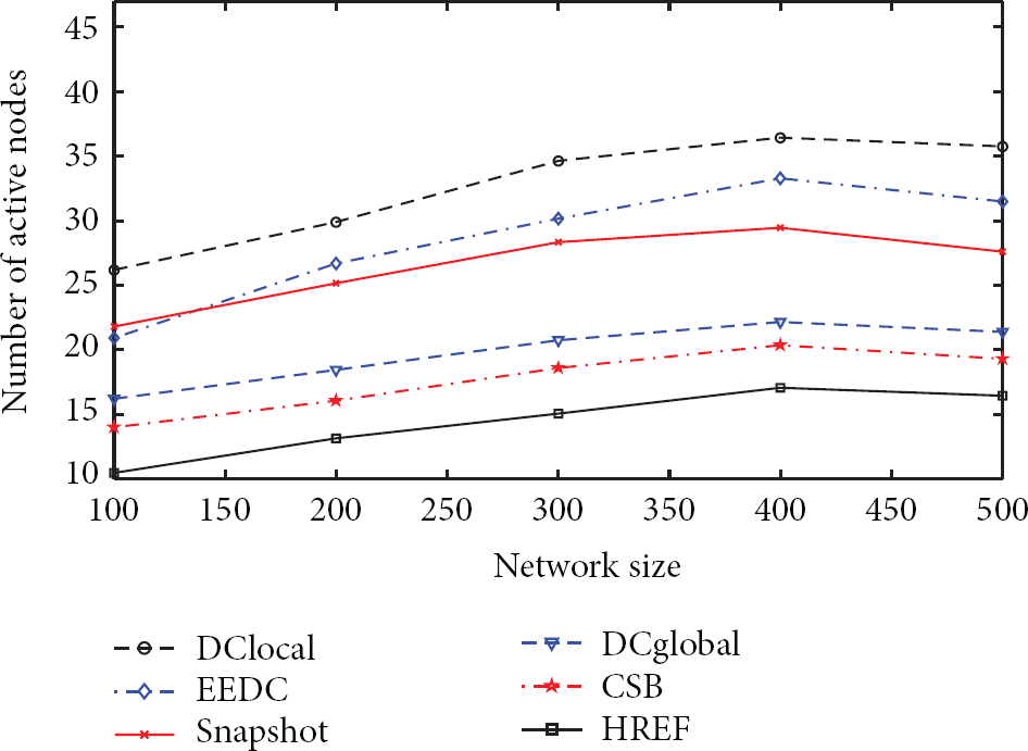
The impact of network size on the number of active nodes.

HREF always has better performance compared with CSB, as we can see from Figure 2. For example, the number of active nodes selected by HREF is only 80.91% of that by CSB in case that the network size is 300. It demonstrates that HREF is rather significant to reduce the active nodes by removing nodes which can be computed by the corresponding correlated node set with the help of CNSC algorithm.

In all cases, HREF and CSB have better performance compared with related algorithms, that is, EEDC, DCglobal, Snapshot, and DClocal. When $n=300$ , the number of selected node is 15.05, 18.6, 20.75, 30.15, 28.35, and 34.65 with HREF, CSB, DCglobal, EEDC, Snapshot, and DClocal.

5.2.2. Impact of Error Threshold

The error threshold varies from 0.1 to 1.15 with increment as 0.15 in the simulations. As shown in Figure 3, the number of active nodes selected by HREF is lower than other algorithms in all cases. As the error threshold increases in the range of [0.1, 0.55], the number of active nodes decreases significantly. However, it is not obvious in the case that the error threshold is larger than 0.7. Hence, it is helpful to reduce the number of active nodes if a larger error threshold is tolerant in some applications.

Figure 3

The impact of error threshold on the number of active nodes.

5.2.3. Impact of the Number of Events

The number of events varies from 5 to 40 with increment as 5 and the simulation result is demonstrated in Figure 4. It shows that the number of selected active nodes is independent of the number of events by using the data computing Formula (2). It can be seen that HREF and CSB have better performance compared with related algorithms regardless of the number of events.

Figure 4

The impact of the number of events on the number of active nodes.

5.3. Comparison of Network Lifetime

There are variations of measurement for network lifetime [27], such as the first node to die, the number of alive nodes, and the fraction of alive nodes. The measurement with the first node to die is not a good measure metric in practical applications, especially in the dense-deployed wireless sensor networks. This is because the redundancy among correlated nodes is helpful to illuminate the defect of single-node failure. The definition based on fraction of alive nodes regards that the network is alive when the fraction of surviving nodes remains above a given threshold [32]. The network lifetime is defined in this paper as the time period during which the fraction of alive nodes remains above a given threshold and they are also connected.

To measure the network lifetime, we have to determine the relay nodes forwarding the sensing data from active nodes by constructing a minimum Steiner tree [33]. The nodes selected by the minimum Steiner tree construction step are called Steiner nodes. Note that the relay nodes do not need to sense data. In the following experiments, we compared the network lifetime of our algorithms to related algorithms in various environmental parameters.

5.3.1. Impact of Network Size

The network size is set from 100 to 500 with increment as 100, and the simulation result is demonstrated in Figure 5. It shows that the network lifetime increases along with the network size increasing. This is reasonable because the number of selected nodes might be independent on the network size. When there is enough data redundancy among the sensing data, more redundant nodes are used to extend the network lifetime, as shown in Section 5.2.1, HREF and CSB have better performance compared with related algorithms regardless of network size. Especially, our algorithm works better when the network size is larger than 200.

Figure 5

The impact of network size on the network lifetime.

The HREF has significant improvement on the network lifetime compared with CSB too. For example, the lifetime has about 18.19% increment compared with CSB in case that the network size is 300. It is reasonable since we adopt not only node reduction but also node replacement strategies which are rather helpful to enlarge the network lifetime.

5.3.2. Impact of Error Threshold

The error threshold varies from 0.1 to 1.15 with increment as 0.15 in the simulations. As shown in Figure 6, the network lifetime increases along with the error threshold increasing. HREF and CSB have better performance compared with the related algorithms, that is, EEDC and DCglobal. CSB has a better performance compared with DCglobal especially when the error threshold is larger than 0.4. The network lifetime of HREF algorithm is longer than the other algorithms in all cases.

Figure 6

The impact of error threshold on the network lifetime.

5.3.3. Impact of Interval

The value of interval varies from 20 to 160 with increment as 20 in the simulations. In Figure 7, the network lifetime increases along with the interval when it is smaller than 80. However, this trend slows down when interval is large than 80. It means that it benefits to extend the network lifetime if a larger interval is tolerant in some applications. In addition, HREF and CSB have better performance compared with related algorithms regardless of the interval.

Figure 7

The impact of interval on the network lifetime.

5.3.4. Impact of Fraction of Alive Nodes

The fraction of alive nodes varies from 0.6 to 1 with increment as 0.05 in the simulations. In Figure 8, the network lifetime decreases along with the fraction of alive nodes increasing. The HREF has better performance compared with related algorithms. The network lifetime of CSB is longer than that of DCglobal when the fraction of alive nodes is smaller than 0.95. However the case changes when the fraction of alive nodes is larger than 0.95. This is because CSB balances between the data coverage range priority and the energy priority. As the data coverage range priority prefers to select nodes with larger data coverage ranges, these nodes with lower energy might be selected as well, which results in rapid node failure and a dying network. The similar conclusion is drawn in Section 3.1. However, as the measurement of the first node to die is not suitable measure metric for network lifetime evaluation in practical applications, the CSB is still better than DCglobal in this case.

Figure 8

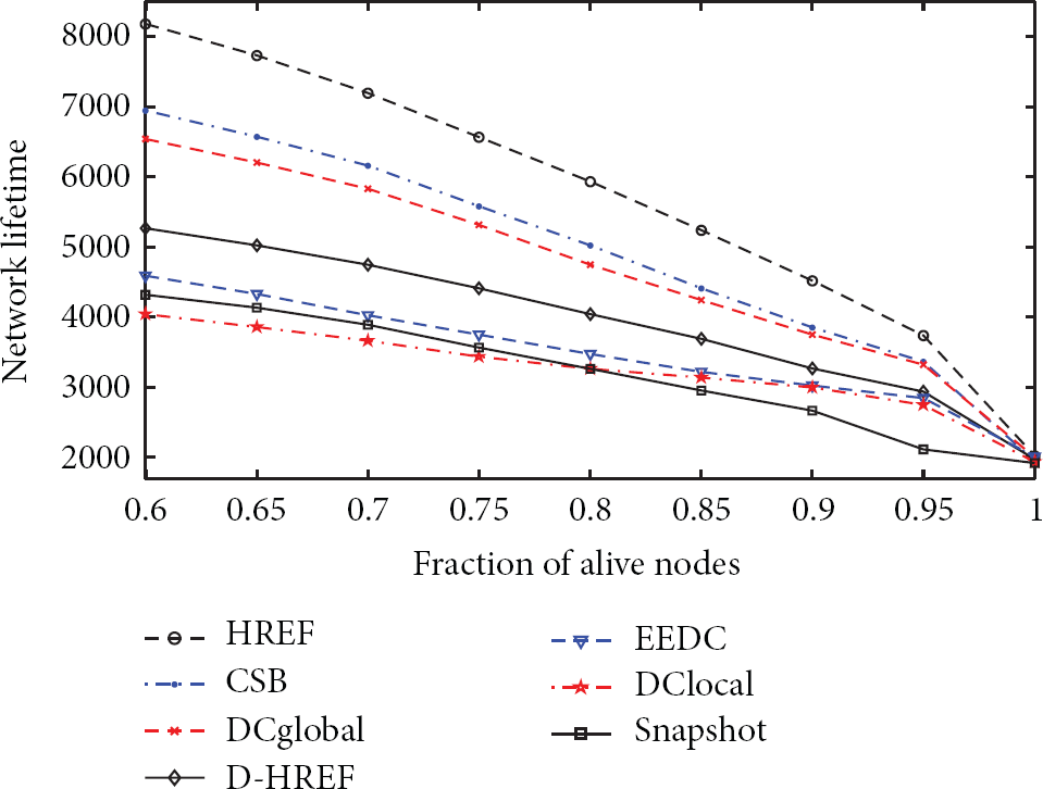
The impact of the fraction of alive nodes on the network lifetime.

5.3.5. Impact of Number of Events

The number of events varies from 5 to 40 with increment as 5 and the simulation result is demonstrated in Figure 9. It shows that network lifetime is independent of the number of events. However, HREF and CSB have better performance compared with related algorithms regardless of the number of events.

Figure 9

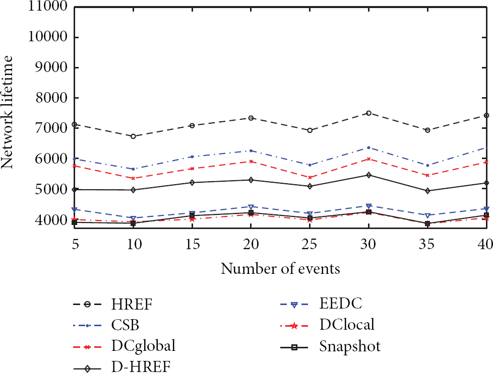
The impact of the number of events on the network lifetime.

6. Related Works

Energy efficiency is a critical design consideration in battery powered and densely deployed wireless sensor networks, which can be achieved by minimizing the number of messages transmitted during the data collection process. Related works include clustering, network coding, in-network data aggregation, and approximate data collection.

Clustering is proven to be an effective approach to provide better data aggregation and scalability for large wireless sensor network [6–11]. Recently, Aslam et al. [7] propose a novel multicriterion optimization technique based on energy-efficient clustering approach. This method takes multiple individual metrics as inputs in the cluster head selection process and simultaneously optimizes the energy efficiency of each individual node as well as the overall system. Karaboga et al. [8] propose an energy-efficient clustering mechanism based on artificial bee colony algorithm to prolong the network lifetime. The simulation results show that the artificial bee colony algorithm based clustering approach can be applied to routing protocols successfully. Naeimi et al. [9] classify routing protocols according to their different objectives and methods by addressing both the shortcomings and the strength of clustering process on each stage of cluster head selection, cluster formation, data aggregation, and data communication and summarized them into categories. Moreover, Lloret et al. demonstrated in [10] that cluster-based mechanisms allow multiple types of network topologies in order to have the most efficient network. Lehasini et al. [11] used clusters to improve the network coverage.

In-network data aggregation [12–18] is another approach to reduce the amount of data transmitted by the nodes and prolong the network lifetime. It performs data aggregation in network to reduce the amount of data transmission by constructing a routing tree. In [12, 13] we can find complete surveys on distributed database management techniques and data aggregation for wireless sensor networks. Al-Karaki et al. [14] present a Grid-based Routing and Aggregator Selection Scheme (GRASS), which achieves low-energy dissipation and low-latency without sacrificing quality. Seyin et al. [15] propose a localized and energy-efficient data aggregation tree approach called Localized Power-Efficient Data Aggregation Protocols (L-PEDAPs) for sensor networks. Gao et al. [16] jointly adopt the cooperative multiple-input-multiple-output and data-aggregation techniques to reduce the energy consumption per bit in wireless sensor network by reducing the amount of data for transmission and better using network resources through cooperative communication.

Approximate data collection is also an energy-efficient approach which is further divided into two subcategories. The first subcategory is approximate data collection via probabilistic models of sensing data collected from wireless sensor networks [19, 20]. Xua and Choi [19] propose a new class of Gaussian processes for resource-constrained mobile sensor networks and propose a distributed algorithm which achieves the field prediction by correctly fusing all observations. Min and Chung [20] present an approximate data gathering approach which utilizes temporal and spatial correlations for wireless sensor network and does not transmit the data to the sink if the data are accurately predicted. The second subcategory is approximate data gathering without probabilistic models. Kotidis [23] propose Snapshot queries for energy-efficient data acquisition in sensor networks. They constitute a network Snapshot through selecting a set of active nodes which is used to provide quick approximate answers to user queries and reducing the energy consumption substantially in wireless sensor network. Gupta et al. [28] design techniques that exploit data correlation among nodes to minimize communication costs incurred during data gathering in a wireless sensor network. They design distributed algorithms that can be implemented in an asynchronous communication model. They also design an exponential approximation algorithm that returns a solution within $O(\log n)$ of the optimal size. Liu et al. [24] propose a data collection approach based on a careful analysis of the sensor data. By exploring the spatial correlation of sensing data, they dynamically divide the nodes into clusters such that the sensors in the same cluster have similar sensing time series which can share the workload of data collection since their future data may likely be similar. Hung et al. [22] propose an algorithm to determine a set of active nodes with high residual energy and wide data coverage ranges. Here, the data coverage range of a node is the set of nodes that have sensor data very close to the particular node. They also develop an algorithm to further reduce the extra cost incurred in messages collection and transmission for selection of active nodes.

In previous work, we have studied the minimum-latency data aggregation problem and proposed a new efficient scheme for it [34]. The basic idea is that we first build an aggregation tree by ordering nodes into layers and then we proposed a scheduling algorithm on the basis of the aggregation tree to determine the transmission time slots for all nodes in the network with collision avoiding. We have proved that the upper bound for data aggregation with our proposed scheme is bounded by $(15R+\mathrm{\Delta }-15)$ for wireless sensor networks in two-dimensional space, where $\mathrm{\Delta }$ is the maximum degree and R is the network radius. We have also simulated the case in three-dimensional wireless sensor networks and proposed an aggregation tree construction algorithm based on maximum independent set [35]; the height of the spanning tree can be reduced to about 50%.

In previous work, we study the node selection problem with data accuracy guaranteed in service-oriented wireless sensor networks [36]. We exploit the spatial correlation between the service data and aim at selecting minimum number of nodes to provide services with data accuracy guaranteed. Firstly, we have formulated this problem into an integer nonlinear programming problem to illustrate its NP-hard property. Secondarily, we have proposed two heuristic algorithms, namely, Separate Selection Algorithm (SSA) and Combined Selection Algorithm (CSA). The SSA is designed to select nodes for each service in a separate way, and the CSA is designed to select nodes according to their contribution increment.

7. Conclusions

Due to the correlation and redundancy among the sensing data in wireless sensor networks, it is an important issue to develop an energy-efficient active node selection strategy, which not only improves the network lifetime but also is helpful to solve other problems, such as lower network throughput and serious node conflict in dense wireless sensor networks. In this paper, we concern with the active node selection issue and provided a formal definition for this problem. We propose the Cover Sets Balance (CSB) algorithm and High Residual Energy First nodes selection (HREF) algorithm aiming at extending the network lifetime of wireless sensor networks. We also propose a Correlated Node Set Computing (CNSC) algorithm to find the correlated node set for a given node. Experimental results on synthesized data sets show that HREF can significantly reduce the number of active nodes, and these algorithms are able to significantly extend the network lifetime compared with related works. In the future work, we are to further consider the temporal correlation among the sensing data and design an efficient node scheduling scheme with both spatial and temporal correlation.