Sage Journals: Discover world-class research

Abstract

Flow induced vibration due to the dynamics of rotor-stator interaction in an axial-flow pump is one of the most damaging vibration sources to the pump components, attached pipelines, and equipment. Three-dimensional unsteady numerical simulations were conducted on the complex turbulent flow field in an axial-flow water pump, in order to investigate the flow induced vibration problem. The shear stress transport (SST) k-ω model was employed in the numerical simulations. The fast Fourier transform technique was adopted to process the obtained fluctuating pressure signals. The characteristics of pressure fluctuations acting on the impeller were then investigated. The spectra of pressure fluctuations were predicted. The dominant frequencies at the locations of impeller inlet, impeller outlet, and impeller blade surface are all 198 Hz (4 times of the rotation frequency 49.5 Hz), which indicates that the dominant frequency is in good agreement with the blade passing frequency (BPF). The first BPF dominates the frequency spectrum for all monitoring locations inside the pump.

1. Introduction

For a water pump, the pressure fluctuation and unsteady dynamic forces induced by the complex and rotating inner turbulent flow are one of the main reasons causing vibration of pump components and hydraulic noises. With the more and more applications of pumps, the unstable operation problem caused by hydraulic excitation has been becoming increasingly prominent. Due to its crucial impact on pump design and operations, the investigation of pressure fluctuations in pumps is of continuous interest.

In the past, many experimental and numerical investigations have been carried out to capture the unsteady interactions between turbulent flow and solid structures in pumps and investigate the frequency characteristics of pressure fluctuations. The fast Fourier transform (FFT) method was often used to obtain the spectra of pressure fluctuations as a function of position and flow rate in the posttest data analysis [1]. Parrondo-Gayo et al. [2] investigated the unsteady pressure distribution existing in the volute of a conventional centrifugal pump by means of four piezoresistive pressure transducers mounted at 36 locations around the front side of the volute casing. Their experiments demonstrated a strong increase in the magnitude of dynamic forces and dipole-like sound generation in off-design conditions. It is principally a consequence of the interaction of nonuniform outflux from impeller to tongue [3, 4]. Barrio et al. [5] presented a study on the fluid-dynamic fluctuations in a centrifugal pump with different radial gaps between the impeller and the volute. For a given impeller diameter, the dynamic load increases for off-design conditions, especially for the low range of flow rates, whereas the progressive reduction of the impeller-tongue gap brings about corresponding increments in dynamic load. Wang and Tsukamoto [6] conducted a study on the unsteady phenomena under the off-design conditions of a diffuser pump. Solis et al. [7] studied numerically the influence of splitter blades and radial gap on the reduction of pressure fluctuation levels at the blade passage frequency in a volute type centrifugal pump. They employed unsteady Reynolds averaged Navier-Stokes (URANS) approach to solve the unsteady flow and pointed out the fact that assuming the flow close to a fully developed condition at outlet provides better results concerning the pressure amplitude levels. Spence and Amaral-Teixeira [8] explored the characteristics of pressure pulsations in a centrifugal pump, measuring in various positions the pulsations levels and finding strong amplitudes at the impeller outlet. Majidi [9] investigated by numerical simulations the unsteady periodic behavior of the flow in a classic pump, noticing that the flow was characterized with pressure fluctuations due to the interaction between the impeller and the volute casing.

Nowadays, the often used study approaches to pressure fluctuation caused by unsteady turbulent flow are computational fluid dynamics (CFD) numerical calculations, flow field measurement techniques such as particle image velocimetry, laser Doppler velocimetry, and so on, and signal test of pressure fluctuation. The flow field in an axial-flow pump, however, is difficult to be measured due to rotor-stator interaction. Thus, CFD numerical simulation technique, which has been testified to be a powerful and efficient way to study the characteristics of pressure fluctuation in water pumps, can be employed to resolve the internal turbulent flow field in the axial-flow pumps. In this paper, the three-dimensional (3D) unsteady turbulent flow in the full passage of a model axial-flow water pump was simulated using CFD technique, through which the pressure fluctuation characteristics at the locations of inlet and outlet of the impeller and the blade were studied. The obtained information from such investigations can be provided for further optimal design of the axial-flow pump, which is the motivation of the present study.

2. Numerical Simulation Procedures

2.1. Computational Domain and Conditions

The simulated target is an axial-flow water pump. Figure 1 shows a 3D solid perspective of the model pump. The inlet flow rate is Q_m = 305 kg/s; the head is H = 29.5 m; the rotating speed is n = 2970 rpm. The blade passing frequency $f = Z_{i} (n / 60)$ (where n,Z, and i are the rotating speed, the number of blades, and harmonic orders, respectively) of this model pump is calculated to be 198 Hz (the rotation frequency of 49.5 Hz multiplied by the number of blades).

Figure 1:

3D solid perspective of pump and sketch of the pump structured mesh.

The entire hydraulic passage of the model axial-flow pump was taken as the computational domain. In order to minimize the effects of boundary conditions and ensure numerical stability, appropriate extensions were processed at the inlet and outlet pipes. The inlet pipe of the solution domain is located approximately at the upstream of the inducer blade leading edge with 5 times the hydraulic radius; the outlet pipe is also roughly 5 times the hydraulic radius. The whole computational domain was divided into five zones including the inlet pipe, inducer, impeller, exit guide vane, and outlet pipe. Structured hexahedral cells were used to define all domains (Figure 1). Relatively fine grids were used near the hub, shroud, and blade surfaces, as well as near the leading and trailing edges. The resulting grid size used during the numerical simulations was determined after a grid independence analysis on the total head, with a simulation carried out in the steady regime. Finally, approximately 1.35 × 10⁶ cells were used for the numerical simulations, which assured no influence on the numerical results. The time step corresponds to the time when the rotator passes one degree, which is 5.61167 × 10⁻⁵'s.

2.2. Numerical Methods

Numerical simulations of the turbulent velocity field and pressure fluctuations in the axial-flow water pump model were carried out using a commercial CFD code, CFX. The finite volume method was used for the discretization of governing equations (continuity equation and momentum equation) in the space region. A constant axial velocity based on the mass-flow rate was specified at the inlet. The outlet was set as outflow boundary condition. The no-slip conditions for the boundary layers were imposed over walls. Due to the rotation of impeller, two interfaces between the rotor and stator were formed, one of which was between the inducer and the impeller, and the other was between the impeller and exit guide vane. In the steady calculations, based on the so-called multiple reference frame model, the inlet pipe, outlet pipe, inducer, and exit guide vane were set in stationary frame, while the impeller was set in rotary frame. The unsteady simulation was initialized from the solution of a steady calculation, whereby it was not performed until the steady convergence was reached. For the unsteady calculation, the sliding mesh technique was applied to simulate the rotor-stator interaction. The interfaces between two stationary components, rotary and stationary components, were set as general grid interface and rotor/stator interface, respectively. As for the discretization in the time domain, the second-order implicit format was adopted. The pressure-velocity coupling was performed using the SIMPLEC algorithm. Second-order format was used for pressure term and QUICK format for other terms. The criterion for convergence was considered to be 10⁻⁴, allowing an optimal number of iterations for each time step.

2.3. SST k-ω Turbulence Model

The unsteady flow was simulated using the shear stress transport (SST) k-ω model. The use of a k-ω formulation in the inner parts of the boundary layer makes the SST k-ω turbulence model directly usable all the way down to the wall through the viscous sublayer; hence, the SST k-ω model can be used as a low-Reynolds-number turbulence model without any extra damping functions [10]. The SST k-ω formulation also switches to k-ε behavior in the free stream and thereby avoids the common k-ω problem that the model is too sensitive to the inlet free stream turbulence properties. The SST k-ω model does produce a bit too large turbulence levels in regions with large normal strain, like stagnation regions and regions with strong acceleration, but this tendency is much less pronounced than that with a normal k-ε model. The transport equations for k and ω are as follows:

\begin{matrix} \frac{\partial (ρ k)}{\partial t} + \frac{\partial (ρ U_{j} k)}{\partial x_{j}} = \frac{\partial}{\partial x_{j}} [(μ + \frac{μ_{t}}{σ_{k}}) \frac{\partial k}{\partial x_{j}}] + P_{k} - β^{'} ρ k ω, \\ \frac{\partial (ρ ω)}{\partial t} + \frac{\partial (ρ U_{j} ω)}{\partial x_{j}} = \frac{\partial}{\partial x_{j}} [(μ + \frac{μ_{t}}{σ_{ω 1}}) \frac{\partial ω}{\partial x_{j}}] + (1 - F_{1}) 2 ρ \frac{1}{σ_{ω 2} ω} \frac{\partial k}{\partial x_{j}} \frac{\partial ω}{\partial x_{j}} + α_{1} \frac{ω}{k} P_{k} - β ρ k ω^{2}, \\ F_{1} = \tanh (ar g_{1}^{4}), \\ ar g_{1} = \min (\max (\frac{\sqrt{k}}{β^{'} ω y}, \frac{500 ν}{y^{2} ω}), \frac{4 ρ k}{C D_{k ω} σ_{ω 2} y^{2}}), \\ C D_{k ω} = \max (2 ρ \frac{1}{σ_{ω 2} ω} \frac{\partial k}{\partial x_{j}} \frac{\partial ω}{\partial x_{j}}, 1.0 \times 1 0^{- 10}), \\ μ_{t} = \frac{ρ α_{2} k}{\max (α_{2} ω, S F_{2})}, \\ F_{2} = \tanh (ar g_{2}^{2}), \\ ar g_{2} = \max (\frac{2 \sqrt{k}}{β^{'} ω y}, \frac{500 ν}{y^{2} ω}) . \end{matrix}

(1)

If Φ₁,Φ₂, and Φ₃ stand for k-ω turbulence model, k-ε turbulence model, and SST turbulence model, respectively, then Φ₃ = F₁Φ₁ + (1-F₁)Φ₂. In the above equations, y is the distance from the wall, ν is kinematic viscosity, P_k is the production rate of turbulence, and S is the strain rate tensor.

3. Results and Discussions

The total head predicted by SST k-ω turbulence model is slightly smaller than the design value, with discrepancy of only 3.4%. From this point of view, we can conclude that the rotating turbulent flow inside the simulated axial-flow water pump obtained with SST k-ω model is credible, and it can be used to analyze the internal pressure fluctuations induced by unsteadiness of the flow. Monitoring points for pressure fluctuations in the axial-flow model pump are shown in Figure 2.

Figure 2:

Monitoring points in the axial-flow pump. The 3 monitoring points P01–P03 are located at the impeller inlet from hub to shroud; P04–P06 are at the impeller outlet from hub to shroud; P07–P09 and P16–P18 are on the pressure and suction surfaces of the impeller blade near the inlet from hub to shroud, respectively; P10–P12 and P19–P21 are on the pressure and suction surfaces of the impeller blade in the middle from hub to shroud, respectively; P13–P15 and P22–P24 are on the pressure and suction surfaces of the impeller blade near the outlet from hub to shroud, respectively.

3.1. Analysis on Time Domain of Pressure Fluctuations

In the simulation of unsteady flow, the pressure fluctuation coefficient is defined by $C_{p} = (p - \bar{p}) / 0.5 ρ u^{2}$ , where p is the static pressure of monitoring points, $\bar{p}$ is the average static pressure, and u is the circumference speed of impeller. Figure 3 shows the time domain of calculated C_p on 3 monitoring points (P01–P03) at the location of impeller inlet. The pressure fluctuation amplitude is the largest at the monitoring point P02, a little smaller at P01 near the hub, and the smallest at P03 near the shroud. At the location of impeller outlet, as shown in Figure 4 for the time domain of calculated C_p on 3 monitoring points P04–P06, the pressure fluctuation amplitude is the largest at the monitoring point P04 near the hub and gradually decreases from the hub to the shroud (from P04 to P06). Comparing Figure 3 with Figure 4, it can be found that the pressure fluctuation amplitude at the impeller inlet is almost twice larger than that at the impeller outlet.

Figure 3:

Time domain of pressure fluctuation at the location of impeller inlet.

Figure 4:

Time domain of pressure fluctuation at the location of impeller inlet.

Figure 5 shows the time domain of pressure fluctuations on the pressure surfaces of the impeller blade. P07, P08, and P09 are monitoring points located near the inlet of impeller from hub to shroud; P10, P11, and P12 are in the middle between inlet and outlet; P13, P14, and P15 are near the outlet of impeller. It can be seen from Figure 5 that the amplitude of pressure fluctuations decreases from impeller inlet to impeller outlet, which means that the impact from the upstream flow decreases gradually. Meanwhile the amplitude of pressure fluctuations also decreases from hub to shroud for the 3 monitoring stations.

Figure 5:

Time domain of pressure fluctuation on the pressure surface of the impeller blade.

Figure 6 shows the time domain of pressure fluctuations on the suction surface of the impeller blade. P16, P17, and P18 are monitoring points located near the inlet of impeller from hub to shroud; P19, P20, and P21 are in the middle between inlet and outlet; P22, P23, and P24 are near the outlet of impeller. Overall, the amplitude of pressure fluctuations slightly increases from impeller inlet to impeller outlet. It means that the pressure fluctuation on the suction surface could be influenced by some factor produced by the turbulent flow and the influence of such factor increases from the upstream to the downstream. The vortex structure is the key element in any turbulent flows. Thus, we can naturally speculate that such influencing factor could be the vortex structures formed in the rotating turbulent flow in the simulated axial-flow pump. The vortex structures in the exit guide vane are then extracted by means of the Q-method [11], as shown in Figure 7. It can be seen that there are many coherent vortex structures in the exit guide vane region, which are rotating and unsteady with time (as visualized from the time-series animation, not provided here). The vortex structures in the exit guide vane influence the interface between the impeller and exit guide vane, which is transmitted to the domain of impeller.

Figure 6:

Time domain of pressure fluctuation on the suction surface of the impeller blade.

Figure 7:

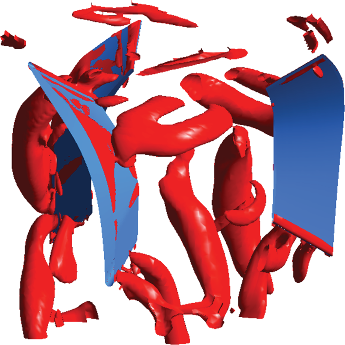
Extracted turbulent vortex structures in the exit guide vane.

3.2. Analysis on Frequency Domain of Pressure Fluctuations

The frequency domain (spectrum) of pressure fluctuations on each monitoring point is calculated by FFT. Figure 8 shows the frequency spectrum of pressure fluctuation at the location of impeller inlet. The x-coordinate of Figure 8 (also Figures 9 and 10) is the relative frequency normalized with the rotation frequency of 49.5 Hz and so represents the number of rotation rounds. Since the number of impeller blade is 4, the flow frequency and its harmonics caused by impeller are 4 times (so-called blade passing frequency, BPF) the rotational frequency and its harmonics, respectively.

Figure 8:

Frequency spectrum of pressure fluctuation at the location of impeller inlet.

Figure 9:

Frequency spectrum of pressure fluctuation at the location of impeller outlet.

Figure 10:

Frequency spectrum of pressure fluctuation on the pressure surface of the impeller blade.

The energy amplitude of pressure fluctuation is the largest on the monitoring point P02 at impeller inlet, smaller on P01 near the hub, and the smallest on P03 near the shroud. Due to the interaction of rotor and stator, the energy amplitude of pressure fluctuations at impeller outlet from the rim to hub is different from the impeller inlet, as shown in Figure 9. At impeller outlet, the energy amplitude of pressure fluctuation is the largest on the point P04 near the hub, smaller on P06 near the shroud, and the smallest on P05. Overall, the energy amplitude of pressure fluctuations at impeller outlet is smaller than that at impeller inlet. Meanwhile, low-frequency (less than 1 Hz) spectrum at impeller outlet becomes pronounced, as compared with that at impeller inlet. This phenomenon should be caused by the shedding of vortex structures in the exit guide vane, as shown in Figure 7, which can be transmitted to the domain of impeller.

Figure 10 shows the frequency spectrum of pressure fluctuation on the pressure surface of the impeller blade. Clearly, the dominant flow frequency caused by impeller is also the BPF. Similar to that happened to the impeller outlet, the energy amplitudes of pressure fluctuations at low frequencies (lower than the BPF) on the pressure surface of impeller blade are pronounced as well (Figure 10). Again, such phenomenon should also be caused by the coherent vortex structures existing in the rotating turbulent flow. Figure 11 shows an example of vortex structures in the impeller region extracted by means of the Q-method. The shedding of the complex vortices in the impeller region may result in additional pronounced pressure fluctuations at low frequency other than the dominant frequency. Similar phenomena can be seen on the suction surface of the impeller blade, as shown in Figure 12.

Figure 11:

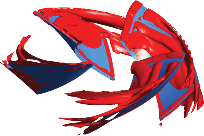
Vortex structures in the impeller region extracted by means of Q-method.

Figure 12:

Frequency spectrum of pressure fluctuation on the suction surface of the impeller blade.

The numerical simulation results about the characteristics of pressure fluctuations induced by the turbulent flow field in an axial-flow pump as elucidated above are of great importance in the optimal design of the pump as well as understanding the dynamics of the interactions between rotating turbulent flow and solid structure, and between rotor and stator. In addition to the energy of pressure fluctuation at the blade passing frequency (which is inevitable in the impeller driven pump), the spectrum at low frequencies on the impeller blade surface and at the impeller outlet induced by turbulent vortices is also obtained in the present calculations. One of the focuses during the optimal design of the pump should be, for example, on the modifications of impeller blade geometry, number of blades, arrangement of blades (such as changing attack angle), and so forth, in order to eliminate those vortex structures or weaken the strength of vortices.

4. Conclusions

Numerical simulations of the rotating turbulent flow in an axial-flow water pump have been carried out based on the Reynolds-averaged momentum equations and SST k-ω turbulence model. The pressure fluctuation characteristics at several typical locations, including the inlet and outlet of impeller and on the pressure and suction surfaces of impeller blade, are then particularly analyzed in time domain and frequency domain. The following main conclusions are drawn from this study.

The maximum amplitude of pressure fluctuation is in the middle between hub and shroud and the minimum is near the shroud at impeller inlet. At impeller outlet, the pressure fluctuation amplitude is the largest near the hub and decreases from the hub to the shroud.

Pressure fluctuation on the impeller blades decreases from hub to shroud. The presence of vortex structures has influences on the pressure fluctuation near the impeller outlet.

The dominant flow frequency, and in consequence the dominant frequency of pressure fluctuations, at the impeller inlet and outlet is the BPF, which equals 198 Hz (4 times of the rotation frequency 49.5 Hz). The energy amplitude of pressure fluctuation at impeller outlet is pronounced at low frequency smaller than the blade passing frequency as well, which is caused by the vortex structures existing in the rotating turbulent flow.

Conflict of Interests

The authors declare that there is no conflict of interests regarding the publication of this paper.

References

Lee

S.-H.

Wang

Y.-Q.

, and Song

J.-I.

, “Fourier and wavelet transformations application to fault detection of induction motor with stator current,” Journal of Central South University of Technology, vol. 17, no. 1, pp. 93–101, 2010.

Parrondo-Gayo

J. L.

González-Pérez

, and Fernández-Francos

, “The effect of the operating point on the pressure fluctuations at the blade passage frequency in the volute of a centrifugal pump,” Journal of Fluids Engineering, Transactions of the ASME, vol. 124, no. 3, pp. 784–790, 2002.

Dong

Chu

, and Katz

, “Effect of modification to tongue and impeller geometry on unsteady flow, pressure fluctuations, and noise in a centrifugal pump,” Journal of Turbomachinery, vol. 119, no. 3, pp. 506–515, 1997.

Choi

J.-S.

McLaughlin

D. K.

, and Thompson

D. E.

, “Experiments on the unsteady flow field and noise generation in a centrifugal pump impeller,” Journal of Sound and Vibration, vol. 263, no. 3, pp. 493–514, 2003.

Barrio

Parrondo

, and Blanco

, “Numerical analysis of the unsteady flow in the near-tongue region in a volute-type centrifugal pump for different operating points,” Computers and Fluids, vol. 39, no. 5, pp. 859–870, 2010.

Wang

and Tsukamoto

, “Experimental and numerical study of unsteady flow in a diffuser pump at off-design conditions,” Journal of Fluids Engineering, Transactions of the ASME, vol. 125, no. 5, pp. 767–778, 2003.

Solis

Bakir

, and Khelladi

, “Pressure fluctuations reduction in centrifugal pumps: influence of impeller geometry and radial gap,” in Proceedings of the ASME Fluids Engineering Division Summer Conference (FEDSM '09), pp. 253–265, Denver, Colo, USA, August 2009.

Spence

and Amaral-Teixeira

, “Investigation into pressure pulsations in a centrifugal pump using numerical methods supported by industrial tests,” Computers and Fluids, vol. 37, no. 6, pp. 690–704, 2008.

Majidi

, “Numerical study of unsteady flow in a centrifugal pump,” Journal of Turbomachinery, vol. 127, no. 2, pp. 363–371, 2005.

10.

Menter

F. R.

, “Two-equation eddy-viscosity turbulence models for engineering applications,” AIAA Journal, vol. 32, no. 8, pp. 1598–1605, 1994.

11.

Zhong

Huang

T. S.

, and Adrian

R. J.

, “Extracting 3D vortices in turbulent fluid flow,” IEEE Transactions on Pattern Analysis and Machine Intelligence, vol. 20, no. 2, pp. 193–199, 1998.