Evolutionary Optimization Algorithms for Sunlight-Based Positioning Sensor Networks

Abstract

The sunlight intensity-based global positioning system (SGPS) is able to geolocate outdoor objects by means of the sunlight intensity detection. This paper presents the integration of SGPS into a sensor network in order to improve the overall accuracy using evolutionary algorithms. Another contribution of the paper is to theoretically solve both global and relative positioning of the sensors composing the network within the same framework without satellite-based GPS technology. Results show that this approach is promising and has potential to be improved further.

1. Introduction

Nowadays global positioning is taken for granted and even more since the arrival of smart phones. However, the unique acceptable solution so far is the global positioning system (GPS) based on satellites [1]. Although it demonstrates a good accuracy, the main drawbacks of this system are often ignored. First, it is government-dependent so there is not any guarantee that it will always be publicly available.

Second, GPS are vulnerable to solar storms. As a matter of fact, the US Government reported that the solar storm which occurred in early March 2012 affected satellites communications “http://www.gps.gov/news/2012/03/solarstorm/ (Sep., 2013).” Although the solar activity of the following years is not expected to be that intensive, this still represents a serious threat for the GPS. In fact, the US Department of Homeland Security has carried out a study of the risks to US critical infrastructure from global positioning system disruptions “http://www.gps.gov/news/2013/06/2013-06-NRE-public-summary.pdf (Sep., 2013).” This serves as enough motivation to investigate satellite-independent global positioning systems.

Many different, satellite-independent approaches have been proposed: measuring sunlight intensity, irradiance, temperature, or magnetic field (see next section for a detailed state of the art). The accuracy of these systems is often hundreds of kilometers. Although none of them are yet a real substitute to satellite-based GPS, many applications could benefit from sunlight-based positioning methods: weather monitoring, ocean tides and wildlife tracking, and extraplanetary location. For example, current environmental research uses GPS-based wireless sensor networks to measure temperature, light, pollution, oceans temperature, tides, and so forth. However, the GPS limits the battery life so it is necessary to change the batteries every few days. This is especially challenging and expensive in wildlife and marine environments. The use of sunlight-based systems in sensor networks (or standalone intelligent sensors) would allow the system to run for months (or even years) without battery replacement.

In this paper, we focus on the sunlight-intensity based global positioning system (SGPS) presented in [2, 3]. SGPS is a novel global positioning system based on sunlight intensity detection able to provide the earth coordinates of an static object, without any GPS-based component by measuring the sunlight intensity of one day, with the only input of the date. The main advantage of SGPS (and most of the sunlight-based systems) is its low power consumption. It can run for months of years with a set of regular batteries. Or even small solar cells could be used as both power source and light intensity sensor. On the other hand, these systems suffer from a low positioning accuracy, limiting their practical uses.

Therefore, the research exposed in this paper aimed to enhance its accuracy by combining it with sensor networks. As this is the first approach to such problem, we focus on networks in which the distances among nodes are known [4]. This integration is able to solve three different problems using the same framework: $(1)$ relative positioning of the nodes in the network: for the case of WSN, this is a very active research field during the last years [5, 6]; $(2)$ global positioning of the nodes in the earth: in the literature this is done by GPS-based systems, where at least one of the nodes of the network has an integrated GPS or cellular-based localization system [7]; $(3)$ improvement of the positioning accuracy of the SGPS as a standalone system: the sensor network is built exclusively to improve the SGPS accuracy.

Although the tendency is to use wireless sensor networks (WSN), wired networks have been extensively applied in industry [8] and other fields [9, 10]. Also, hybrid configurations have been already proposed [11]. Along this paper we are assuming any kind of sensor network since we are focusing on how to combine data from different nodes.

The proposed framework, identified with the acronym SGPSNet, includes a probabilistic model of the error of SGPS, which allows us to compensate it by combining the individual SGPS results of the different nodes with the geometry of the sensor network.

The paper is organized as follows: next section provides the state of the art of satellite-independent geopositioning. In Section 3 the SGPS is introduced. Section 4 analyzes the error of the SGPS. Then, the SGPSNet framework is detailed in Section 5. Experimental setup is described in Section 6 and results and discussion are in Section 7. Finally, the conclusions are presented in Section 8.

2. State of the Art

Satellite-independent geopositioning systems have been studied for several years. The results obtained in terms of positioning accuracy have been a challenge [12]. However, it has been successfully applied to some problems, such as wildlife migratory movements tracking [13]. In fact, many interesting improvements were suggested. Sunrise and sunset times can be identified more accurately by taking into account the temperature together with the light intensity [14] since the temperature signal is more stable. Kalman filters help to decrease the positioning error through the days [15] when the object to geolocate is moving. A simple motion model is given, namely, the maximum distance a specific animal could travel in one day. Therefore, results are corrected when they are in conflict with the motion model.

Ekstrom [16] propose a complex analysis of the twilight for a template-fitting based approach to irradiance data with an estimation of the error [17].

The influence of weather, topography, and vegetation on the light intensity and its measurement have been studied [18]. Therefore, by combining sunlight intensity sampling with other sensors (altitude, humidity, atmospheric pressure, etc.) the location accuracy could be improved.

Other approaches to GPS-less geolocation have been also proposed. For instance, a simple webcam can be used to estimate geolocation by analyzing picture brightness [19, 20]. The magnetic field of the earth has been also tested as a mean to automatically geolocate objects [21, 22].

Statement of Contributions. A probabilistic error model for the SGPS is computed, which is a first in this field. Then, a methodology to combine SGPS solutions from different nodes within a sensor network taking into account an error model is proposed. This allows probabilistically improving the accuracy of the SGPS results for every node. To our knowledge, it is the first time a satellite-based geopositioning system is combined with a sensor network. State-of-the-art approaches are based on initial GPS measurements.

3. System Model

The SGPS is able to geolocate stationary outdoor objects (longitude and latitude coordinates) by measuring sunlight intensity. Since the basis of this system is deeply described in [3], only its outline is included in this paper.

The SGPS operation is presented in Figure 1. In the hardware side, the system is designed to be simple and inexpensive, hence comprising a light sensor and a microprocessor.

Figure 1

SGPS flowchart.

3.1. Sunlight-Based Global Positioning System

The mathematical model of the SGPS relies upon a celestial model which takes into account the rotation and translation movements of the earth. The daylight parameters are influenced by the longitude and latitude coordinates of a given place as shown in Figure 2.

Figure 2

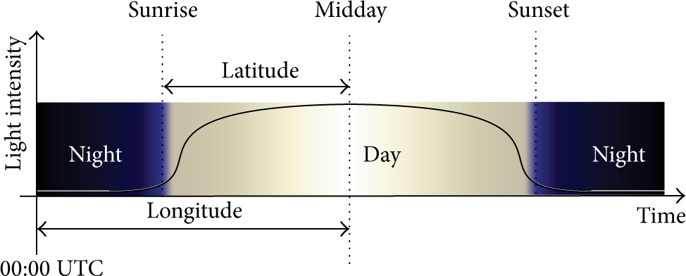
Schema of the mathematical model of the SGPS.

Hereafter, the following convention is going to be employed: times are measured in decimal hours, in the range from 0 to 23.99, and referred to the Coordinated Universal Time (UTC), avoiding daylight saving time issues. Days will be referred to from 1 to 365 (or 366 in a leap year) and angles are expressed in radians. Coordinates are given in radians. Degrees are only shown in the results in order to help the reader in interpreting them. For the longitude the range is from −180° to 180° with the zero reference in the Greenwich meridian and positive coordinates to the east. In the case of the latitude, the range is from −90° to 90° where zero represents equator and positive coordinates represent north.

From the sunlight intensity measurements for a given day d, the sunrise and sunset times ( $t_{\mathrm{sr}}$ and $t_{\text{ss}}$ , resp.) are identified (see Section 3.2). Therefore, the solar noon, $t_{\text{md}}$ , for that day is simply

$$\begin{array}{cc}& t_{\text{md}}=\frac{t_{\mathrm{sr}}+t_{\text{ss}}}{\mathrm{2}}.\end{array}$$

(1)

If $t_{\text{md}}<t_{\text{ss}}$ a fractional day occurs in which the sunset actually happened in the previous UTC day. In these cases, the computed $t_{\text{md}}$ corresponds to the midnight time. To solve this problem, the real noon time $t_{\text{md}}^{\prime }$ for a day d is approximated as follows:

$$\begin{array}{cc}& t_{\text{md}}^{\prime }=\mathrm{mod}\left(t_{\text{md}}+\mathrm{12,24}\right),\end{array}$$

(2)

where $\mathrm{mod}$ refers to the module operation.

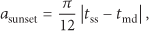
The next step is to compute the angular sunset $a_{\text{ss}}$ ,

$$\begin{array}{cc}& a_{\text{sunset}}=\frac{\pi }{\mathrm{12}}\left|t_{\text{ss}}-t_{\text{md}}\right|,\end{array}$$

(3)

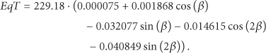
and the declination of the sun δ, approximated by a Fourier series [23]:

$$\begin{array}{l}\delta =\mathrm{0.006918}-\mathrm{0.399912}\cos \left(\beta \right)\\ \hspace{1em}+\mathrm{0.070257}\sin \left(\beta \right)-\mathrm{0.006758}\cos \left(\mathrm{2}\beta \right)\\ \hspace{1em}+\mathrm{0.000907}\sin \left(\mathrm{2}\beta \right)-\mathrm{0.002697}\cos \left(\mathrm{3}\beta \right)\\ \hspace{1em}+\mathrm{0.00148}\sin \left(\mathrm{3}\beta \right),\end{array}$$

(4)

where β is the fractional year, computed as

$$\begin{array}{cc}& \beta =\frac{\mathrm{2}\pi }{\mathrm{365}}d.\end{array}$$

(5)

Finally, the coordinates of the object can be obtained [24]. For the longitude λ,

$$\begin{array}{cc}& \lambda =\mathrm{2}\pi \frac{\mathrm{12}-t_{\text{md}}}{\mathrm{24}},\end{array}$$

(6)

and the latitude φ can be computed by numerically solving the following equation:

$$\begin{array}{cc}& \cos \left(a_{\text{sunset}}\right)=\frac{\sin \left(-\mathrm{0.0145}\right)-\sin \left(\delta \right)\sin \left(\phi \right)}{\cos \left(\delta \right)\cos \left(\phi \right)}.\end{array}$$

(7)

Note that these formulae are well known in astronomy. They are usually applied in a “forward” fashion, known as sunrise equation [24]. That is, given longitude and latitude, compute the sunrise and sunset times. In this case, we are solving the “inverse” problem, which is not trivially solved from the sunrise equation.

It is important to note that sensors usually work with UTC-referred civil times. However, SGPS celestial model is based on solar times. The conversion is straightforward:

$$\begin{array}{cc}& t_{\text{civil}}=t_{\text{solar}}+EqT,\end{array}$$

(8)

where $EqT$ refers to the equation of time. Concretely, the Spencer $EqT$ expression [23] is employed since it uses only information about the day d:

$$\begin{array}{l}EqT=\mathrm{229.18}·\left(\phantom{\left(\mathrm{2}\beta \right)}\mathrm{0.000075}+\mathrm{0.001868}\cos \left(\beta \right)\right.\\ \hspace{1em}\hspace{0.17em}\phantom{\text{hhhhhhhhhh}}-\mathrm{0.032077}\sin \left(\beta \right)-\mathrm{0.014615}\cos \left(\mathrm{2}\beta \right)\\ \hspace{1em}\hspace{0.17em}\left.\phantom{\text{hhhhhhhhhh}}-\mathrm{0.040849}\sin \left(\mathrm{2}\beta \right)\right).\end{array}$$

(9)

3.2. Experimental Results

In order to test the system with real measurements, data from the National Oceanic and Atmospheric Administration (NOAA) public FTP server “ftp://aftp.cmdl.noaa.gov/data/radiation/surfrad (August, 2013)” has been employed. In this case, a simple zero-crossing algorithm is enough to accurately detect the sunrise and sunset times. Also, the sunlight intensity value chosen was determined by using data only from two different days. This ensures a worst-case scenario since more sophisticated methods could be employed. In fact, the sunlight intensity cannot be negative but, due to the hardware employed, inverse currents provoke measures to be negative during night-time. This is the critical point of the system in terms of accuracy. However, the objective of this study is to improve accuracy by other means, since a deeper study of detecting sunrise and sunset is very hardware-dependent.

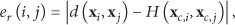
Figure 3 shows the results of the SGPS in a statistical way. They represent the current state of the art of sunlight-based geolocation. Note that these results contain data for almost every day during 10 years along 6 different stations. Although how different conditions affect the system has not been deeply evaluated, results show that they do not have a high impact on the error. How different conditions affect the system has not been evaluated. Clouds, for instance, affect the maximum sunlight value and therefore the rate of change of measures sunlight. However, at sunrise/sunset times there is still enough light to measure. Actually, results show that there were very few days in which the relative error is excessively high. Histograms for latitude and longitude relative errors are shown, computed as

$$\begin{array}{cc}& e_{\text{latitude}}\%=\frac{e_{\text{latitude}}}{\mathrm{180}}\mathrm{100},\hspace{1em}\hspace{1em}{e}_{\text{longitude}}\%=\frac{e_{\text{longitude}}}{\mathrm{360}}\mathrm{100}.\end{array}$$

(10)

Figure 3

System relative error histograms.

4. SGPS Error Analysis and Modeling

One critical part of the system in terms of accuracy is the sunrise and sunset detection. A bias of several minutes can result in error of hundreds of kilometers. Since it is not possible to accurately predict the error introduced by sunrise and sunset times, the error of the system is modeled in probabilistic terms. Note that the error model (and hence the rest of the framework) is hardware-independent because of the SGPS mathematical model. For a given calibration, it is not possible to have a larger error in longitude than latitude since they are highly correlated. Only the parameters of the error model would vary by sensor calibration. In any case, we are showing a worst-case scenario in which results are shown with a trivial calibration.

If all the errors of the previous experiments are merged and referred to as the global reference frame instead of their local frame (corresponding station), they can be plotted as a dispersion chart, as shown in Figure 4. Analyzing this plot, it is possible to see that latitude error is much larger than longitude error. However, a dispersion pattern is observed: errors are concentrated about the $(\mathrm{0,0})$ point. The farther we get from the origin, the less errors are found. This suggests that the error can be modeled by a standard bidimensional Gaussian distribution:

$$\begin{array}{cc}& f\left(\mathbf{x}\right)=\frac{e^{(-(\mathrm{1}/\mathrm{2}\left)\right(\mathbf{x}-\mathit{\mu }{)}^T{\mathbf{\Sigma }}^{-\mathrm{1}}(\mathbf{x}-\mathit{\mu }))}}{\mathrm{2}\pi {\left|\mathbf{\Sigma }\right|}^{\mathrm{1}/\mathrm{2}}},\end{array}$$

(11)

where $\mathit{\mu }$ is the means vector, representing the average value of the errors in both longitude and latitude, and $\mathbf{\Sigma }$ is the covariance matrix $(2\times 2)$ , symmetric and positive definite, giving the dispersion values in both axes. The variable is the vector composed of a pair longitude-latitude $\mathbf{x}=(\text{long},\text{lat})$ . Both $\mathit{\mu }$ and $\mathbf{\Sigma }$ are computed using standard methods.

Figure 4

Dispersion chart of the error and its Gaussian probabilistic model.

The parameters of the fitting (covariance matrix and means vector) depend on the hardware and signal processing techniques used during the measurement and sunrise and sunset identification processes.

5. SGPS Network Integration

The error model described in the previous section suggests that using more than one sensor to measure may improve the accuracy. In this fashion, errors can be decreased by combining the distance among two or more sensors with the output of the SGPS algorithm for each node.

The algorithm described in the following paragraphs aims to be integrated within any kind of sensor network. This paper focuses on networks in which the distances among nodes are known or can be accurately computed. It is also assumed that the nodes of the network are measuring sunlight intensity throughout all the day. In order to be as general as possible, let us assume that the localization is not the main task of the network, but it is required (e.g., data geotagging). Therefore, SGPS algorithm will run “in the background.” Network nodes will independently sample sunlight intensity throughout the day, from 00 hours UTC until 23.99 hours UTC. Once the day has finished, every node will analyze the data to identify sunrise and sunset times. For this, we employed a zero-crossing algorithm as detailed in Section 3.2. Note that this can be done in an online fashion so that no data is required to be stored. Longitude and latitude are computed for every node according SGPS formulae described in Section 3. Then, the SGPS solutions are combined probabilistically with the objective of improving the location estimates.

In case of an infrastructure-less network, where there is a lack of a central controller, one of the nodes could temporally act as central node in order to carry out the SGPS solution combination. As it will be explained, the proposed optimization algorithm is only based on summations and multiplications (also the optimization method chosen), meaning it does not require high computational capacity. Besides, the algorithm does not require to be computed in real time. Therefore computational limitations are not a problem. Also, the optimization parameters could be highly optimized in order to reduce the number of computations required in order to save energy.

5.1. Formulation as an Optimization Problem

The proposed approach formulates the problem as an optimization trying to minimize two factors: $(1)$ distance error among sensors and $(2)$ deviation of the candidate solution with respect to the initial SGPS location. Let us consider the scenario shown in Figure 5, composed of three nodes. “SGPS initial result” is the nonoptimized calculated position, while “candidate solution” is the optimized position.

Figure 5

Parameters influencing the fitness function evaluation for a given candidate solution ( $H_{\mathrm{1,3}}$ omitted for clarity).

Let us suppose a sensor network with n nodes, with a real distance among nodes $i,j$ of $d\left({\mathbf{x}}_i,{\mathbf{x}}_j\right)=d\left({\mathbf{x}}_j,{\mathbf{x}}_i\right)$ for all $i,j$ , which we assume to be known. The set of coordinates of the node i of the sensor network is denoted as ${\mathbf{x}}_i=(\text{lon}{\text{g}}_i,\text{la}{\text{t}}_i)$ . Consequently, ${\mathbf{x}}_{S,i}$ is the set of coordinates of the initial solution of the SGPS for that node. ${\mathbf{x}}_{c,i}$ is the candidate solution for every node i. Intuitively, the farther a candidate solution goes from the initial SGPS solution, the less likely it is (given the proposed error model). Therefore, we will use the Mahalanobis distance $D_M({\mathbf{x}}_{S,i},{\mathbf{x}}_{c,i})$ to compute the distance between the initial SGPS solution and the current candidate solution for node i. It computes the distance between two random variables subject to the same probability distribution: the probabilistic error model in our case, defined by $(\mathit{\mu },\mathbf{\Sigma })$ computed in Section 4. It is computed as follows:

$$\begin{array}{cc}& D_M\left({\mathbf{x}}_{S,i},{\mathbf{x}}_{c,i}\right)=\sqrt{{\left({\mathbf{x}}_{S,i}+{\mathbf{x}}_{c,i}-\mathit{\mu }\right){\mathbf{\Sigma }}^{-\mathrm{1}}\left({\mathbf{x}}_{S,i}+{\mathbf{x}}_{c,i}-\mathit{\mu }\right)}^T}.\end{array}$$

(12)

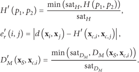
Since the error model is centered at ${\mathbf{x}}_{S,i}$ , $D_M({\mathbf{x}}_{S,i},{\mathbf{x}}_{c,i})$ expresses in terms of distance how likely the location of ${\mathbf{x}}_{c,i}$ is. The objective of the addition of the Mahalanobis distance is keeping the candidate solutions in the most probable places according to the error model.

On the other hand, let us define the distance error $e_r(i,j)$ as the comparison between the real distances between nodes $i,j$ and the distances of the candidate solutions for those nodes:

$$\begin{array}{cc}& e_r\left(i,j\right)=\left|d\left({\mathbf{x}}_i,{\mathbf{x}}_j\right)-H\left({\mathbf{x}}_{c,i},{\mathbf{x}}_{c,j}\right)\right|,\end{array}$$

(13)

where $H({\mathbf{x}}_{c,i},{\mathbf{x}}_{c,j})$ means the Haversine distance between candidate solutions for two different nodes. The Haversine is defined as the shortest distance between two points on a sphere expressed in terms of longitudes λ and latitudes φ. Using the earth's parameters (distances in kilometers and angles in degrees), the Haversine distance is computed as follows:

$$\begin{array}{cc}& H\left(p_{\mathrm{1}},p_{\mathrm{2}}\right)=\mathrm{6372.8}\times \mathrm{2}\times \text{atan}\mathrm{2}\left(\sqrt{h},\sqrt{\left(\mathrm{1}-h\right)}\right),\end{array}$$

(14)

where h is

$$\begin{array}{cc}& h=\sin {\left({\phi }_{\mathrm{2}}-{\phi }_{\mathrm{1}}\right)}^{\mathrm{2}}+\cos \left({\phi }_{\mathrm{1}}\right)\cos \left({\phi }_{\mathrm{2}}\right)\sin {\left({\lambda }_{\mathrm{2}}-{\lambda }_{\mathrm{1}}\right)}^{\mathrm{2}}.\end{array}$$

(15)

Finally, the following fitness function is defined:

$$\begin{array}{cc}& f={\displaystyle \sum }_{i=\mathrm{0}}^n‍\left(\alpha D_M\left({\mathbf{x}}_{S,i},{\mathbf{x}}_{c,i}\right)+\left(\mathrm{1}-\alpha \right){\displaystyle \sum }_{\forall j\ne i}‍e_r\left(i,j\right)\right).\end{array}$$

(16)

Intuitively, this fitness function is a weighting (with α as weighting factor) between the Mahalanobis distance among candidate locations and original SGPS locations and the total error of the distances nodes.

The magnitude orders of the components of the fitness function are different. The distance errors are usually around hundreds or thousands of kilometers. The Mahalanobis distance could reach such orders of magnitude, but once the optimal solution is being reached it is usually less than 1. Then, saturation is applied in order to ensure that outliers are not decisive when evaluating the fitness function. The saturation levels $\text{sa}{\text{t}}_H$ and $\text{sa}{\text{t}}_{D_M}$ are experimentally chosen because they enormously depend on the error model parameters. Once saturated, the fitness parameters are normalized to be between 0 and 1. Thus,

$$\begin{array}{l}{H}^{\prime }\left(p_{\mathrm{1}},p_{\mathrm{2}}\right)=\frac{\min \left(\text{sa}{\text{t}}_H,H\left(p_{\mathrm{1}},p_{\mathrm{2}}\right)\right)}{\text{sa}{\text{t}}_H},\\ e_r^{\prime }\left(i,j\right)=\left|d\left({\mathbf{x}}_i,{\mathbf{x}}_j\right)-H^{\prime }\left({\mathbf{x}}_{c,i},{\mathbf{x}}_{c,j}\right)\right|,\\ D_M^{\prime }\left({\mathbf{x}}_S,{\mathbf{x}}_{c,i}\right)=\frac{\min \left(\text{sa}{\text{t}}_{D_M},D_M\left({\mathbf{x}}_S,{\mathbf{x}}_{c,i}\right)\right)}{\text{sa}{\text{t}}_{D_M}}.\end{array}$$

(17)

Finally, the objective is to find the set of coordinates for all the nodes ${\mathbf{X}}_c=〈{\mathbf{x}}_{c,\mathrm{1}},\dots ,{\mathbf{x}}_{c,n}〉$ that minimizes:

$$\begin{array}{l}\underset{{\mathbf{X}}_c}{\min }J\left({\mathbf{X}}_c\right)\\ \hspace{1em}={\displaystyle \sum }_{i=\mathrm{0}}^n‍\left(\alpha D_M^{\prime }\left({\mathbf{x}}_{S,i},{\mathbf{x}}_{c,i}\right)+\left(\mathrm{1}-\alpha \right){\displaystyle \sum }_{\forall j\ne i}‍e_r^{\prime }\left(i,j\right)\right).\end{array}$$

(18)

Among all the existing optimization methods, the differential evolution (DE) algorithm [25] has been chosen. More specifically an implementation optimized to solve large-scale problems [26]. This choice is not critical in the performance, since a low computational time is not an objective. However, DE has proved to work efficiently in many applications [27] so it is robust enough to provide good results for the proposed approach.

6. Differential Evolution Algorithm Setup

In order to test the validity of the proposed optimization model, a subset of days among the NOAA database have been chosen, which are common for all the available stations, displayed in Figure 6. The SGPS algorithm was applied to every node individually and the aforementioned optimization was carried out. The test bench is composed by the application of the algorithm from 3 up to 6 NOAA stations.

Figure 6

Location of the 6 stations used in the experiments.

In the DE algorithm, the latitude and longitude values for every node are introduced as variables to optimize. Therefore, there are $\mathrm{2}n$ variables, where n is the number of stations included. As there is no information about the initial conditions, the first population is created using a uniform distribution within $[-\mathrm{90,90}]$ for latitude and $[-\mathrm{180,180}]$ for longitude. Each candidate, a vector composed of $\mathrm{2}n$ values (n latitudes and n longitudes), is evaluated according the fitness function (18). Longitude coordinates are enforced to lie within −180° and 180°. However, the candidates which have latitude values out of range are assigned an infinite fitness value. For instance, a latitude of 91° is not equivalent to any other latitude, while a longitude of 181° is equivalent to −179°. The population size is set to 100 individuals, with a maximum of 1000 iterations. The DE step size (known as parameter F) is set to 0.7 while the crossover probability (CR) is set to 1. This increases the speed of the optimization for the proposed optimization problem. Finally, the DE strategy employed is DE/local-to-best/1/bin, which means that the mutation takes a random element and the best element of the previous population. This strategy attempts a balance between robustness and fast convergence.

7. Results and Discussion

In first place the Gaussian distribution for the error model is computed as described in Section 4, for the data belonging to the first two years available in the NOAA dataset (1995-1996), totaling 2077 days. In this case the Gaussian is defined by the following parameters (given in degrees):

$$\begin{array}{cc}& \mathit{\mu }=\left|\begin{array}{c}{\mu }_{\text{long}}\\ {\mu }_{\text{lat}}\end{array}\right|=\left|\begin{array}{c}-\mathrm{0.0941}\\ \mathrm{1.8674}\end{array}\right|,\hspace{1em}\hspace{1em}\mathbf{\Sigma }=\left|\begin{array}{cc}\mathrm{2.4024}& \mathrm{0.6757}\\ \mathrm{0.6757}& \mathrm{190.73}\end{array}\right|.\end{array}$$

(19)

The means of the distribution are slightly north-biased since the data available in the NOAA FTP are only from the United States.

In our experiments, we simulated the sensor network using a computer as a central node in order to perform computations. SGPS was independently applied to all NOAA stations, obtaining a set of longitude and latitude estimates. Then, the optimization was proposed in Section 5 for each available day. Therefore, we assumed perfect communication among nodes and the existence of a central node (which can be any of the network nodes).

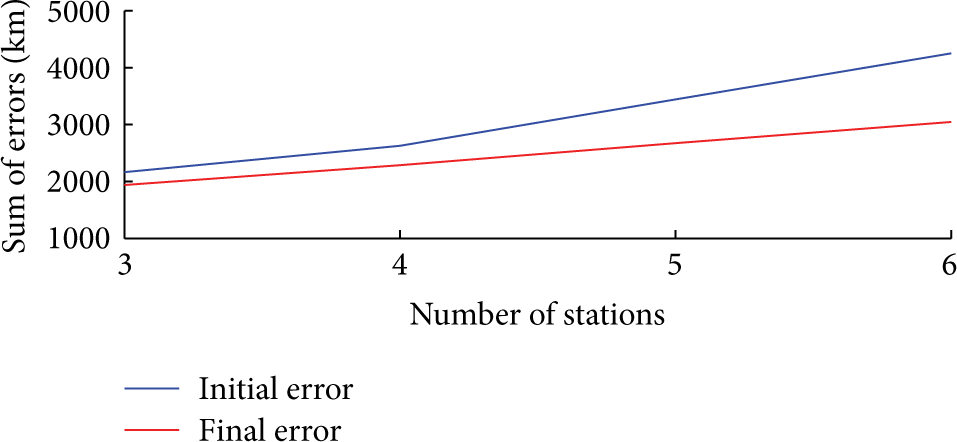
As the optimization procedure is stochastic it is possible for the final results to be worse than the initial results since a lower fitness value does not assure a better final result. Although this would seem counterintuitive, no other variables are available in the optimization. The initial error is considered as the sum for all the nodes of distances between the real locations of the nodes and the SGPS locations. The final error is defined as the sum of the distances between the enhanced locations and the real node locations. Table 1 shows the number of days in which the final results are improved. Figure 7 shows the mean of the initial and final errors plotted against the number of stations.

Table 1

Improvement of the SGPSNet method over the standard SGPS.

Number of stations	Number of days	Number of days improved	Number of days worsened	Improvement	Mean computation time (s)
3	3587	1820	1767	50.7%	22.65
4	2943	1428	1515	48.5%	28.44
5	2180	1273	907	58.4%	35.16
6	1730	1142	588	66%	41.97

Figure 7

Improvement of the means of the errors depending on the number of stations.

As can be seen from Table 1 and Figure 7, the improvement ratio increases with the number of stations. On average, the final error is reduced compared to the initial error. This means that, in case of improvement the accuracy gain is more significant that the worsening in the rest of the cases. Also this improvement increases as more stations are used in the algorithm. In Figure 8 a geometric representation of the results for a specific day is shown. While the final position for station 4 is worsened, stations 3, 5, and 6 are improved. Stations 1 and 2 remained on the surroundings of their initial position.

Figure 8

Geometric representation of the SGPSNet results.

In order to deeply analyze these results, let us divide the year into two different parts: central part, those days between the first equinox ( $d=\mathrm{81}$ ) and the second equinox ( $d=\mathrm{265}$ ), and lateral part, those days between the second equinox ( $d=\mathrm{265}$ ) and the first equinox of the following year ( $d=\mathrm{81}$ ).

In our case, the days in the central part of the year are favored due to the bias of the Gaussian error model. Table 2 and Figure 9 detail the same results as shown before, but only taking into account days of the central part of the year. The improvement ratios are higher. However, Figure 9 shows that the results in the worsened cases (mainly in the lateral part of the year) are almost the same as if no algorithm was applied, since the final error is near to that plotted in Figure 7. One possible solution is to fit two different Gaussian distributions, one for every part of the year. In any case the distribution chosen is enough to prove the validity of the proposed method.

Table 2

Improvement of the SGPSNet method over the standard SGPS on the central part of the year.

Number of stations	Number of days	Number of days improved	Number of days worsened	Improvement
3	1851	1691	160	91.4%
4	1439	1330	106	92.6%
5	1120	1082	38	96.6%
6	793	754	39	95%

Figure 9

Improvement of the means of the errors depending on the number of stations for the central part of the year.

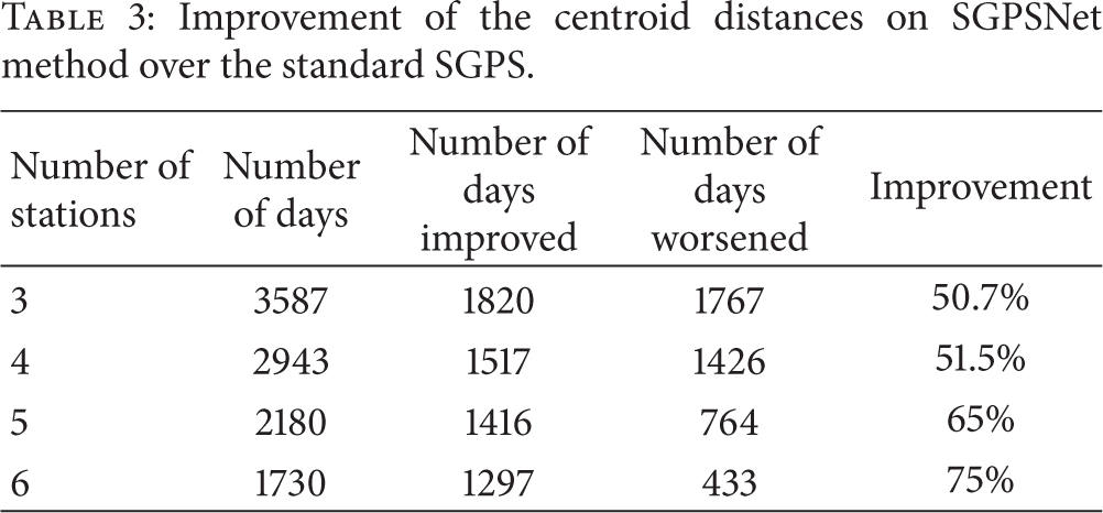
Next, the results are analyzed from the point of view of the centroid of the sensor network. In this case, the initial error is measured as the distance from the centroid of all the independent SGPS solutions to the real centroid. The final error is then computed as the distance from the centroid of all the enhanced SGPS positions to the real centroid. In Figure 10 and Table 3 these errors are depicted for the whole year. As seen in the figure, the final error is much lower for the centroid computed with the enhanced SGPS locations. Intuitively the progression of the graph is expected to decrease linearly, as in Figures 7 and 9. However, a possible explanation is that the same centroid can be obtained from infinite combinations of positions, giving a more stochastic character to these results. Although the proposed method does not explicitly optimize the centroid error, it improves the centroid error really well, which can be worthy to explore in the future work. Table 3 shows the improvement ratio of the centroid distances. Comparing the results with those shown in Table 1, it turns out that the algorithm works better for optimizing the centroid of the stations.

Table 3

Improvement of the centroid distances on SGPSNet method over the standard SGPS.

Number of stations	Number of days	Number of days improved	Number of days worsened	Improvement
3	3587	1820	1767	50.7%
4	2943	1517	1426	51.5%
5	2180	1416	764	65%
6	1730	1297	433	75%

Figure 10

Improvement of the means of the centroid errors depending on the number of stations for all year.

8. Conclusion

Throughout this paper various novelties have been included. First, the error of the SGPS has been modeled as a probabilistic function allowing us to leverage this model in order to improve the accuracy. A novel method based on the application of the SGPS to sensor networks to geolocate the nodes both globally and locally is proposed but focusing on the improvement of the global positioning accuracy. This SGPS-sensor network integration enhances the accuracy of the system by reducing the global positioning error of the SGPS that is also one of the main drawbacks of this system together with the refresh rate of the position. The proposed approach is modeled as an optimization problem. The accuracy is improved stochastically, but, thanks to the DE metaheuristic optimization method, an improvement is guaranteed for most of the cases.

Note that our proposed approach uses SGPS as an underlying system but any method capable of estimating global coordinates for an object fits the SGPSNet formulation. The only requirement is that the error model for those methods should be accurately modeled. Along this paper many assumptions were made. Namely, nodes were far away from each other and distances among them are known. Future work will focus on creating a more general methodology so that it can be applied to smaller networks (in terms of distances among nodes) in which the overlapping among probabilistic error functions is higher. Also, the application to WSN, in which the distances among nodes are unknown and have to be computed online by automatic methods, is one of the main points of the future work.