
Abstract
Structural and industrial environments use hundreds to thousands of bolts to hold parts together. For most mechanical systems, the bolts are critical components because they are subject to axial tension triggering various failures; for example, compromised screw threadsand/or vibration caused untightening. Severe damages can result injury of personnel, equipment damage, and even loss of life. Typically, monitoring mechanical tension of the bolts is visually performed with red dot bolts or manually inspected, but this process is expensive in terms of effort, time, and money; additionally, perhaps the accessibility of the bolt itself is very difficult. Changing this tedious monitoring process to automated, quick, and precise process is our concern in this work. Nowadays, wireless sensor networks (WSN) have wide range of applications especially in surveillance and monitoring systems. In this paper, we propose an efficient and power-aware technique to monitor bolted joints using wireless sensor networks. Also, due to the randomization placement of bolts in real world, our proposed mechanisms have been studied with different deployment node distributions (grid, uniform, normal, and exponential). Furthermore, we have investigated different scenarios with different probability of bolt failures to explore their effect on power consumption and network lifetime.
1. Introduction
Over the past decades, a great advancement has been achieved in wireless sensor networks on both hardware and software. The wireless sensor network consists of spatially distributed autonomous and battery-powered sensors to monitor physical or environmental conditions, such as temperature, sound, vibration, pressure, motion, or pollutants, and working cooperatively to pass their data through the network to a main location (i.e., base station or sink). In recent years wireless sensor networks have been used in a wide range of applications, such as battlefield surveillance, industrial process automation (monitoring and controlling), meteorological areas, home appliances, structural health monitoring (SHM), and human health applications [1]. However, wireless sensor nodes have limited resources in terms of processing, storage, power, and communication capabilities and use existing routing protocols for ad hoc networks is not efficient. Therefore, many power-aware routing protocols have been proposed and several surveys and comparison studies have been conducted [2–7].
These advancement stimulated a lot of attention on the research of structural health monitoring technology [8–12] since it provides a reliable, efficient, and economical approach to increase the safety and to reduce the maintenance costs of engineering structures. These structures range from aging fleets of aircraft and ship structure to civil structures, such as bridges, highways, and tall buildings [13]. Failure of bolted joints can lead to catastrophic events, such as leaking of poisonous material, train derailments, aircraft crashes. Most of these failures occur due to the reduction of the variation of the load, induced by mechanical vibration and temperature or human errors in the assembly or maintenance process [14]. Monitoring bolted joints in one of SHM techniques means developing a technique to reduce the likelihood of failure of structures due to loosening of bolted joints in an accurate way. The monitoring system is mainly targeted for collecting the measurements from sensors deployed within the mechanical structure and storing the measurement data within a central data repository. For guaranteed and reliable measurement and data collection, structural monitoring systems use coaxial wires for communication between sensors and the base station [15]. While coaxial wires provide a very reliable communication link, their installation in structures can be expensive and labor intensive. For example, structural monitoring systems installed in tall buildings have been reported in the literature to cost in excess of $5000 (USD) per sensing channel [16]. As structural monitoring systems grow in size (as defined by the total number of sensors), the cost of the monitoring system can grow faster than at a linear rate. For example, the cost of installing over 350 sensing channels upon the Tsing Ma suspension bridge in Hong Kong is estimated to have exceeded $8 million [15]. The high cost of installing and maintaining wires is not restricted only to civil structures. Others have reported similar issues with respect to the costs associated with monitoring systems installed within aircrafts, ships, and other large structural systems [17].
In this paper, we described our proposed mechanism to automate the process of monitoring bolted joints leading to more accurate and flexible monitoring process at low cost of time, money, and effort. In our smart bolt development we adopted the well-known routing protocol Low-Energy Clustering Hierarchy-Centralized Cluster Formation (LEACH-C) [18] to work with our mechanism. LEACH-C has been selected after conducting several simulations to select either LEACH or LEACH-C; the results showed that LEACH-C is performing better than LEACH in case of smart bolt applications. That is due to its centralized nature of cluster heads selection algorithm, where the base station is responsible for selecting the clusters every round. To verify our proposed mechanism we carried out intensive simulations with different variations of node location distributions, sparse and dense networks, central and corner base stations, day and week scenarios, and finally different probabilities for a bolt to be in poor condition (i.e., bolt tension is less than a predefined threshold). The energy consumption measurements are extracted from real experiments with Arduino sensor platform and injected into NS2 network simulator to enhance the practicality of our simulation. The performance metrics are focused on throughput, energy consumptions, and network lifetime, which are the most important measurements in WSN applications.
This paper is organized as follows; the literature review is introduced in the next section, then a detailed description of the smart bolt monitoring mechanism is followed, after that the simulation setup along with the simulation results analysis and discussion sections is presented, and finally we conclude with some conclusions and suggest future work.
2. Literature Review
A two-tier SHM architecture using wireless sensor network has been proposed by [19]. The proposed monitoring system distributes the monitoring functionality between the ordinary sensors and the cluster servers, where the sensors send the data to the clusters to be processed and analyzed and react based on the results. The system is composed of compact sensors (footprint size of 4–7.5 cm2) using Cygnal microcontroller. The microcontroller properties having 50 mW power consumption, 2 KB of RAM for data storage, and an Ericsson Bluetooth wireless transceiver are used for communication between wireless sensors and wireless data servers, operating on the 2.4 GHz radio band, and Bluetooth radio consuming 35 mW of electrical power. After data are collected by the wireless sensors, data can then be transferred wirelessly to wireless data servers (cluster nodes). Each cluster node has both a short-range radio for communication with wireless sensors in its cluster and a long-range radio for communication with other remote cluster nodes. The central cluster server is designed to both store and process the vast amounts of data collected from the cluster's wireless sensors. The cluster node is designed using a single board computer (SBC) running Microsoft Windows OS. MATLAB is installed in the node for processing measurement data for signs of structural damage. Although this technique provides complete hardware and software solution, the whole system seems to be not scalable and not portable because the cluster nodes are servers with heavy software and have different capabilities than the ordinary sensors.
Another wireless structural monitoring system proposed by researchers at MicroStrain is assembled from off-the-shelf electrical components resulting in a functionally rich platform [20]. At the core of the wireless sensor node is the 8-bit Microchip PIC16C microcontroller where embedded software is stored in the microcontroller's internal electrically erasable, programmable, and read-only memory (EEPROM). To allow for the interfacing of various sensors to the node, the Analog Devices AD7714 16-bit ADC is included in the node design. An attractive feature of the AD7714 ADC is the programmable voltage gain on the sensor inputs ranging from 1 to 128. To achieve wireless communication back to a remote data repository, a surface acoustic wave (SAW) radio operating on the 418 MHz frequency is selected. To modulate digital data upon the selected carrier frequency, the frequency shift keyed (FSK) pulse code modulation method is employed. This pulse code modulation technique permits the wireless nodes to detect errors in the wireless communication channel, thereby increasing the reliability of the radio. When fully assembled, the wireless node is 9 × 6.5 × 2.5 cm3 and is powered by two 1.5 V (3 V total) lithium-ion batteries.
Arms et al. [21] have reported a more recent improvement on the original wireless sensor proposed by [20]. The SAW wireless radio originally integrated with the wireless sensor represents a poor utilization of the wireless channel since only one sensor node can communicate at any one point in time. Instead, Arms et al. proposed the integration of the Chipcon CC1021 wireless transceiver with the wireless node. Operating on the 900 MHz radio band, multiple nodes can utilize the same wireless bandwidth through frequency division multiple access (FDMA) methods. In stark contrast to the original time division multiple accesses (TDMA) methods, the new radio allows 26 wireless sensors to communicate simultaneously on the 26 individual frequencies equally distributed from 902 to 928 MHz.
3. Smart Bolts Monitoring Mechanism
Smart bolt is one application of SHM mechanisms [22] that are used to monitor remote bolted joints and send alerts if any bolt loses its tension beyond a certain threshold. An intensive study on LEACH-C [18] was conducted by Baroudi et al. [23]; it showed that LEACH-C outperforms LEACH and it is suitable to be the routing protocol of our proposed smart bolt monitoring mechanism. LEACH-C is a robust and energy-efficient wireless communication protocol. In our proposed solution, two main mechanisms are developed; the first one is without real-time wakeup clock (RTC) and the second is with RTC. The second one is more efficient in terms of energy consumption; however, it has additional cost of adding the necessary hardware to all sensors (RTC wakeup clock).
3.1. A Brief Description of LEACH-C
LEACH-C uses centralized clustering algorithm where each node sends information about its current location (possibly determined using a GPS receiver) and energy level to the base station (BS). In addition to determining good clusters, the BS needs to ensure that the energy load is evenly distributed among all the nodes. To do this, the BS computes the average node energy, and whichever node has energy below this average cannot be cluster head for the current round. Using the remaining nodes as possible cluster heads, the BS finds clusters using the simulated annealing algorithm to solve the NP-hard problem of finding optimal clusters. This algorithm attempts to minimize the amount of energy for the noncluster head nodes to transmit their data to the cluster head, by minimizing the total sum of squared distances between all the noncluster head nodes and the closest cluster head. Once the cluster heads and the associated clusters are found, the BS broadcasts a message that contains the cluster head ID for each node. If the node's cluster head ID matches its own ID, the node is a cluster head; otherwise, the node determines its TDMA slot for data transmission and goes to sleep until time to transmit data. TDMA schedule is constructed by every cluster head; it is a schedule for its cluster nodes to transmit their data, and so one frame contains a number of slots equal to the number of nodes inside the cluster [18]. Figure 1 illustrates LEACH-C architecture where each bolt is attached to a wireless sensor that senses the tension of the bolt every predefined period of time and sends its readings to the cluster head if it is necessary (beyond certain threshold).
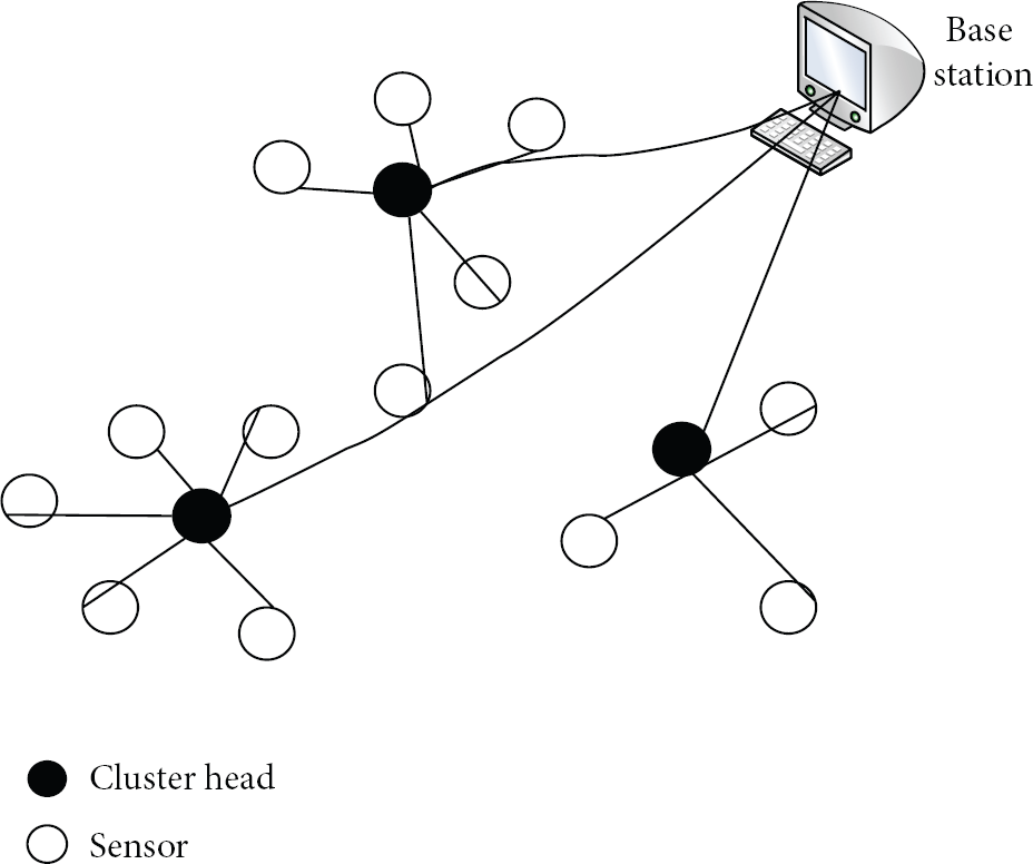
LEACH-C network architecture.
3.2. Smart Bolts without RTC (Sleep Mode)
This special application of monitoring the tension excreted on each bolt does not require extensive data transmissions. In fact, one reading per day is enough. Therefore, two main scenarios are suggested for monitoring the smart bolts: day and week. In the day scenario, each sensor sends one reading per day. The sensor wakes up at specific time each day, reads the bolt tension, sends it to the cluster head, and comes back to sleep mode to minimize energy consumption. The internal clock will trigger the processor to wake up, read, send, and sleep, and so on. Figure 2 depicts the finite state machine (FSM) diagram that illustrates the operations of the smart bolt sensor in the day scenario. Similarly, the cluster head will keep active until all sensor nodes transmit their data and then it aggregates the received data from all its children and sends the aggregated data to the base station and finally it goes to sleep mode. Let TA define the sensor active time slot during each frame and TS define the transmission/reception time; then, we can define the following operation parameters:
Sensor_Active_Time per frame = TA + TS;
Sensor_Sleep_Time per frame = 24 h − Sensor_Active_Time per frame;
C_Head_Active_Time per frame = (TA + TS) * (No. of Children per cluster) + TS;
C_Head_Sleep_Time per frame = 24 h − C_Head_Active_Time per frame.

FSM of the smart bolt sensor nodes in day scenario.
As explained above, considering the nature of the problem, it is not expected that the bolt tension changes daily. Therefore, to save energy, we proposed to report the bolt tension status to the base station every specific period of time (e.g., week, month, etc.). This period of time is determined based on the environment conditions where the smart bolts are deployed. Moreover, within this period the sensor takes multiple readings for bolt tension, and in case this reading exceeds a predefined threshold, it sends alert to its CH; otherwise, it goes again to sleep mode and sends a report at the end of the specified period.
In the following example, we consider the week-period as the necessary time for reporting the status. In the week scenario, the bolt-sensor will send its reading if an abnormal condition is detected (i.e., tension is beyond certain threshold); otherwise, it records the reading and goes to sleep mode again. If the bolt-sensor did not send any data for a week, it will send a report at the end of the week; that means at least one report will be sent per week. To perform this, a timer is adjusted and reinitialized every time the bolt-sensor sends an alert or a report. Figure 3 shows the FSM diagram for the sensor node in case of week scenario.

FSM of the bolt sensor nodes in week scenario.
To simulate the changes in the bolt tension, we assume that the defective nodes are distributed uniformly among the whole network nodes. For example, when we set the abnormal condition to be 0.25, we assume that 25% of the nodes are defective or the node during its lifetime needs to be maintained 25% of this time. Let TA define the sensor active time slot during each frame and TS define the transmission/reception time. Then,
Sensor_Active_Time per Frame = TA + TS * Prob (bolt not in normal condition);
Sensor_Sleep_Time = 24 h − Sensor_Active_Time per frame.
The active and sleep time for cluster head in week scenarios are the same as in day scenarios; that is because the cluster head must be active every day during the frame period expecting either abnormal or weekly reports. Figure 4 illustrates the procedure of week scenario, where AT stands for active time and SPC for sleeping period counter. In week scenarios the maximum period the sensor will not send reports to the cluster head is 7 days, where the sensor sends report even if there is no failure; otherwise, the cluster head will consider it as a dead node.

Week scenario procedure, using sleeping period counter (SPC) with maximum nonsending period of 7 days.
Most of the studies on WSN applications are assuming uniform distribution for the network nodes. However, in most of real applications the sensors might be deployed following different deployment scenarios. Therefore, we used in our simulations different distributions to make our study more realistic. Figure 5 shows the four distributions that we have used in our simulations; Figure 5(b) shows the grid distribution which represents the deterministic distribution and it is used in many WSN applications, for example, agricultural and environmental monitoring applications, due to its high performance, well-organized shape and ease of control. In grid topology, the nodes are placed in such a way where the distance between any two adjacent nodes is the same; that makes clustering calculations easier than random distributions which results in minimizing delay and energy consumption and maximizing network lifetime. Many of WSN applications do not allow deterministic deployment for sensors, such as in disasters and military conditions. In such cases, we use the other distributions such as normal or exponential.

Different deployment distributions with different BS locations: (a) uniform dist., (b) grid dist., (c) normal dist. with μ = 50 and σ = 25, and (d) exponential dist. with λ = 35.
The uniform distribution (Figure 5(b)) has been used in the most of the previous researches. Furthermore, we have added the normal (Figure 5(c)) where the majority of nodes are focused at the center of the field and the exponential distribution (Figure 5(d)) where the majority of the nodes are placed at the corner; the impact of base station location on these distributions has also been studied. For each distribution, we have examined two scenarios, namely, central base station (50, 50) and corner base station (5, 5). In this way we have simulated the all possible combinations of the distributions with base station locations.
3.3. Smart Bolt with RTC (Deep Sleep Mode)
From the sleep mode scenarios, it is clear that most of the energy is consumed during the sleep time. Figure 6 describes an example that clarifies the significant impact of sleep mode on the total energy consumption. In this example we supposed to have a cluster that consists of 3 noncluster nodes (sensors) and one cluster head (CH); the three sensors (S1, S2, and S3) will wake up for small period of time; for example, in case of S1 the period of active time will be AT (S1); in this period it will send the report to the CH and then go back to sleep mode again for long period of time (24 hours-AT (S1)). From our results, as we will see in the results analysis section, 95% of the energy is consumed during the sleep mode, where nearly 0.2 joule is consumed by each sensor per one day.
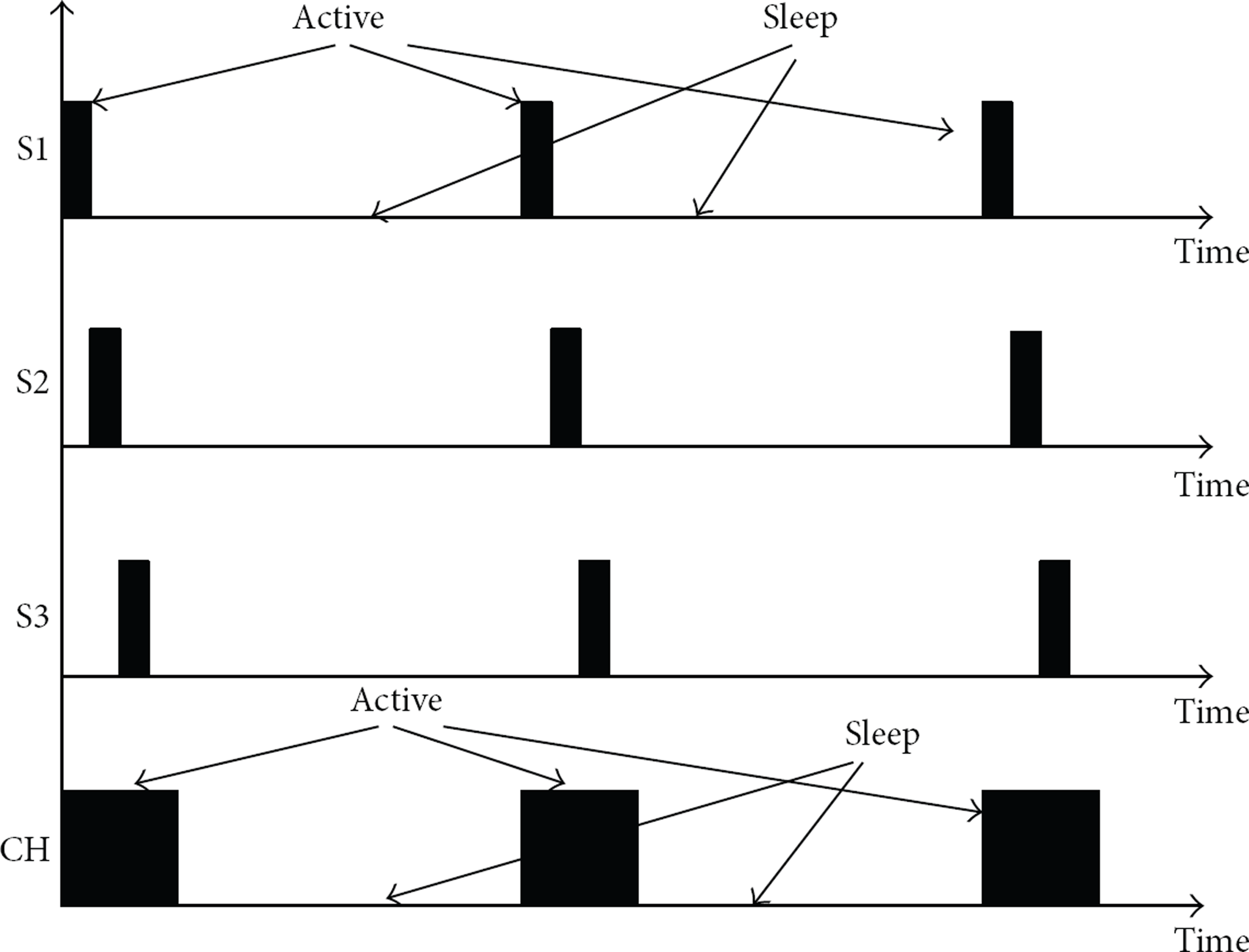
Active and sleep periods in sensors (noncluster heads, S1, S2, and S3) and cluster head (CH).
In this section we propose an enhancement to the smart bolt mechanism by adding a new mode to its sleep modes which was named as deep sleep mode. This enhancement is achieved by adding a real-time wakeup clock (RTC) to each sensor. In this scenario, the processor will alternate between active state and deep sleep where the processor will be almost dead and most of its activities are at hold. Hence, it consumes very little energy. However, to activate the processor again, we need an external interrupt that will be generated by the external clock. From our experiments, we noticed that this clock needs 200 nA to be alive; this value will be added to the current of the sensor in deep sleep mode which is equal to 100 nA, which makes the total 350 nA during deep sleep state, whereas it was 700 nA in the sleep mode scenarios.
In this scenario (deep sleep mode), the sensor and RTC are battery-powered as shown in Figure 7. After the sensor node sends its report to the cluster head, it reschedules its wakeup time and sends it to its RTC which later on will send a wakeup interrupt to the sensor node.

Energy powered node with RTC for wakeup interrupt; INT: interrupt signal, SWT: setting waiting time.
During the active state, the node reads data and processes it to see if it is beyond certain threshold or not. In case the reading exceeds the threshold, it will send a report to cluster head; otherwise, it just issues a command to the RTC on when to wake up next and go back to deep sleep so that more energy is saved. At the specified wake up time, the RTC asserts its interrupt pin, which wakes up the node (based on wake up on interrupt). The node now does any required activity (including synchronization if needed), issue wake up time command to the RTC, and go back to sleep and so on (see Figure 8).
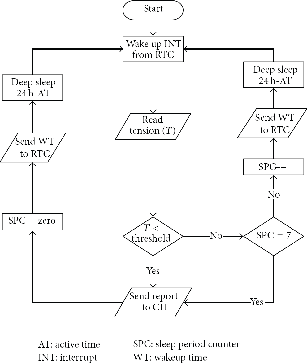
Week scenario with RTC enhancement.
4. Simulation and Results Analysis
The proposed mechanisms have been verified using NS2 simulation, with real energy consumption measurements. We evaluate the proposed mechanisms using the performance metrics as follows:
total energy consumption (Joule/day) which is calculated by computing the total energy consumption of all the network nodes during the whole day, except the base station that is assumed to have unlimited power;
network lifetime (NLT) which is defined as the total time the base station is able to communicate with at least one sensor node (based on the LEACH-C author [18]);
PKT/Joule, which is used to evaluate the energy utilization of the network/protocol. The higher the value, the better the network/protocol.
To ease the presentation of our results, we use the following notations:
CnNd: Leach-c with BS located at the center and normally distributed nodes,
CrNd: Leach-c with BS located at the corner and normally distributed nodes,
CnUd: Leach-c with BS located at the center and uniformly distributed nodes,
CrUd: Leach-c with BS located at the corner and uniformly distributed nodes,
CnEd: Leach-c with BS located at the center and exponentially distributed nodes,
CrEd: Leach-c with BS located at the corner and exponentially distributed nodes,
CnGd: Leach-c with BS located at the center and grid distributed nodes,
CrGd: Leach-c with BS located at the corner and grid distributed nodes.
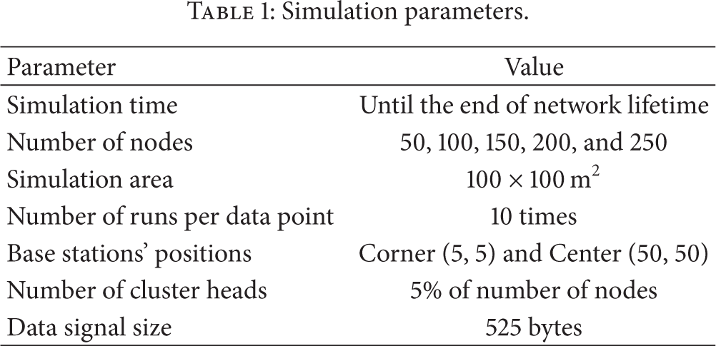
We have used the popular NS-2 simulator [24] to investigate our mechanism. The leach extension (a low-energy protocol simulator for wireless networks) has been integrated with NS using the tools in [25]. For the number of cluster heads in each scenario, we use 5% of the total number of nodes (this is based on LEACH published paper and also recommended by the NS-Leach code documentation). The energy model and other simulation parameters are summarized in Tables 1 and 2. To enhance the fidelity of our results, for each point in our curves, we have developed multiple random topologies for each distribution and then we averaged the collected results.
Simulation parameters.
Energy model parameters.

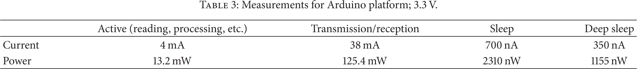
To make our simulations parameters more realistic, we have carried out several experiments on Arduino sensor platform to validate the data sheet energy consumption values during different modes of operation: transmitting/receiving, active and sleep modes. Table 3 presents our findings. These values are injected into NS2 simulator and the code is adapted to work accordingly. Thereby, the results become more meaningful; for example, the network lifetime is calculated by days and years.
Measurements for Arduino platform; 3.3 V.
In the day scenario, the noncluster sensors send one packet per day to the cluster nodes and the cluster head nodes aggregate these data and send them to the base station. As mentioned before, the number of cluster heads is 5% of number of nodes; that makes the average number of nodes per cluster 20. During TDMA phase, the time dedicated by the cluster head for each node to send their data is about 25.2 msec. Thus, approximately one day operation in real time is equivalent to one frame time (20 * slot time, which is 0.5 second) in simulation time.
In Figure 9, we present the day scenario with sleep mode for different sensors deployment strategies at the monitored area on our proposed mechanism. As we mentioned earlier, the deployment strategies that are examined here are the exponential, normal, uniform, and grid distributions; see Figure 5. Starting from the center base station location in Figure 9(a), we use PKT/Joule (packet per joule) measurement to measure the protocol efficiency in utilizing the network energy; it shows that grid and uniform distributions are almost close to each other and outperform the other distributions. In addition, we can observe that the difference in the performance increases as the number of deployed nodes increases. In Figure 9(c), we use J/day (joule per day) measurement which will reflect the total energy consumed per one day which is also a good indication about the network lifetime. And, from the same figure, we can conclude the same as in Figure 9(a), where the uniform and grid distributions still are the best. However, if the base station is located in the corner, the uniform distribution results in Figures 9(b) and 9(d) show the worst performance, which is probably because the base station at the corner is away from many nodes in the network, in contrast to the exponential distribution where most of the network nodes now are close to the base station, which makes it almost the best in case of corner base station location. In average, the grid distribution is the best over all the other distributions in case of sleep mode with packet/day data rate. Furthermore, the figure shows the effect of increasing the number of nodes on the network performance, where we increase the number of nodes in the 100 m2 area from 50 nodes (sparse) to 250 nodes (dense). It is clear that increasing number of nodes degrades the network performance, and that is due to the increasing interference that in turn increases the collisions and packet loss and hence more energy consumption.
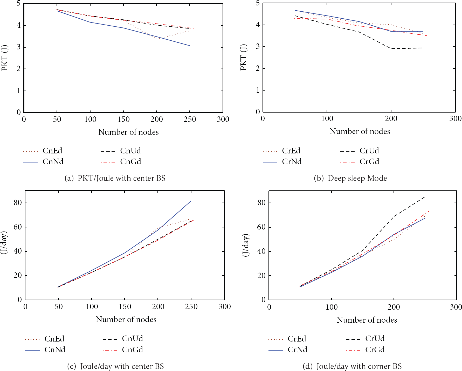
Different distributions deployment and base station location effect on sleep mode mechanism.
It is intuitive that the total energy consumption increases as the number of node increases as shown in Figures 9(c) and 9(d). However, we need to note that most of energy consumption occurs while the sensors are in sleeping mode, where the node consumes nearly more than 95% of its energy during its sleeping period. This approximation is based on the data in Table 3, where the sensor in sleep mode consumes 2310 * (24 hour-slot time) joule which is equal to 0.199 joule per day for each sensor. That means nearly 0.2 joule is consumed per one node every day and if we have 50 nodes, the consumption will be about 10 joule (from calculation) which is nearly the same as in Figure 9(d) plus additional energy that is used in other sensor functions such as sending and receiving. For this reason, the direct extension to enhance this mechanism is to minimize the energy consumption during the sleep period; thereby we came up with the deep sleep mode enhancement as explained above.
Further enhancement in the proposed mechanism is to decrease the amount of data sent to the base station by checking the bolt tension level. If the level is beyond a certain threshold, the sensor is assumed to be malfunctioning and it will send a report to the base station as discussed previously; otherwise, it goes to sleep mode. Figure 10 shows the effect of the likelihood of the bolt on the network performance in terms of PKT/Joule and Joule/day. Four scenarios were simulated; these scenarios are as follows.
Zero%. This is the baseline scenario, where the bolt sensor sends its report every week since the probability of malfunctioning occurrence during the week is zero. (The error means the bolt tension level is normal).
25%. The probability of error occurrence during the week is 25%; when error occurs the sensor will send a report to its cluster head and reset the week counter to zero.
50% and 75%. The same as 25% but with high probability of error occurrence. Of course, 100% represents the day scenario, which means every check (one per day) the sensor will detect an error and sends a report (day scenario).
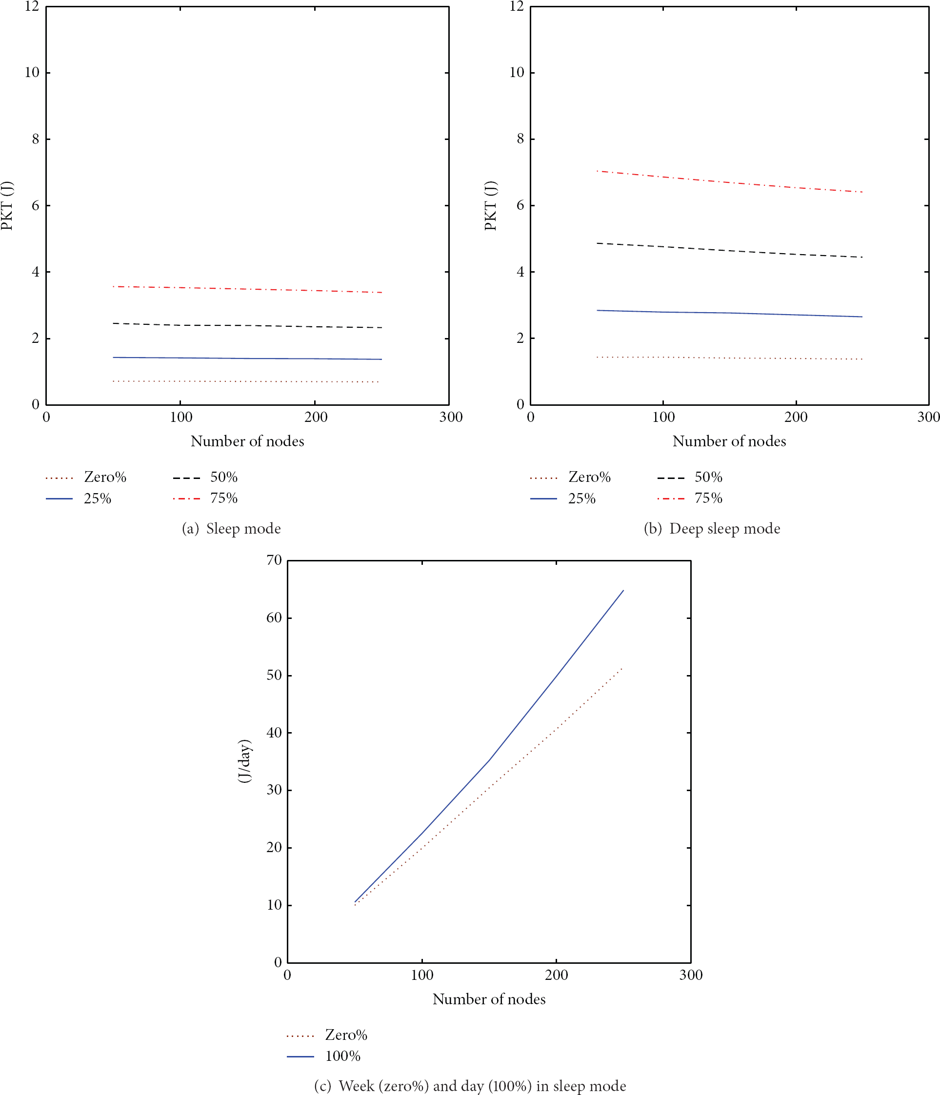
Week scenarios with different error probabilities using uniform deployment.
Figure 10(a) represents the results in sleep mode scenarios; it shows that as the bolt malfunctioning probability increases the packets sent per one joule increases. Comparing to Figure 10(b), the deep sleep mode utilizes the network energy better than sleep mode mechanism. In both cases (i.e., sleep and deep sleep), it is interesting to notice that the amount of packets transmitted per joule is insensitive to the number of nodes in the network. This can be attributed to the fact that the node is most of the time in the sleep/deep mode where the only cause of energy consumption is the internal consumption which makes the denominator very large (i.e., number of packets/total energy). This also explains the linear increase in energy consumption as Figure 10(c). In this figure, we are comparing the energy consumption per day for two extreme cases: the week scenario with perfect normal operation and the week scenario with all nodes malfunctioning, and, hence, they have to report their status every day. In general, as in Figure 10(c), the network lifetime increases as the malfunctioning probability decreases.
Network lifetime (NLT) is a very important measurement in WSN that is used to measure the enhancement in any new WSN algorithm. In Figure 11, we compare our proposed mechanisms in terms of NLT. In these scenarios we use 100 nodes with central base station and the results are taken by averaging 10 random runs’ results. The simulation stops when the number of alive nodes is less than the required cluster heads (5%). Mainly, in this figure we intend to compare the enhancement of deep sleep mode (DSM) versus sleep mode scenarios, where we clearly observe that the network lifetime is doubled for all deployment scenarios. In addition, the week scenarios demonstrated better performance by extending the overall network lifetime. Figures 11(a) and 11(c) show the results of sleep mode mechanism in day and week scenarios, respectively. In general, the week scenario extends the NLT by nearly 60 days (two months) since it sends only one packet per week where it saves the energy of sending and receiving packets during 6 days of the week. As a particular example, Figure 12(a) represents the NLT extension; in case of using uniform distribution the difference was exactly 51 days longer than day scenario. Considering the NLT starting from the first dead node in the network to the last one before the end of the simulation, the day scenario is going faster to the end of NLT than week scenario; that is because the sending rate in day scenario is nearly 7 times faster than week which means the energy consumption is faster. These findings emphasize the impact of energy consumption during the sleep/deep sleep modes for this special application. Therefore, the lifetime extension is fair. On the other hand, the deep sleep mode results, as depicted in Figures 11(b) and 11(d), show very clear enhancement as the NLT in deep sleep scenario is almost doubled compared to the sleep mode scenario. The enhancement of deep sleep mode is clearer in Figure 12(b).

Sleep and deep sleep mode network lifetime (NLT); 100 nodes with perfect operation.

Network lifetime for deep sleep and sleep modes for week/day scenarios under uniform node distribution.
Now, exploring more the NLT behavior of different deployment schemes for the four scenarios (i.e., day, week, SM, and DSM), we can observe the following, in addition to what mentioned above. Firstly, for day scenarios, the behavior of each deployment scenario is clearly distinguished from each other for the whole network life time span. Grid deployment shows the best, followed by the uniform deployment, and then the exponential deployment, and the worst is the normal distribution. Secondly, for the week scenarios, we can still observe the same outstanding performance for grid and uniform distributions for the first 600 days and 1200 days under sleep and deep sleep mode, respectively. However, after that the grid deployment dies quickly compared to other scenarios. This behavior is unexpected, but it can be attributed to the period during for the cluster formation process. It is known that LEACH-C cyclically rebuilds the cluster to ensure uniform energy consumption among all nodes. For week scenarios, the energy consumption during sleep mode is very huge compared to the day scenarios. Therefore, after long operation period, the cluster head nodes will have low energy which may be depleted (i.e., starvation) before the new cluster formation process starts and, hence, the generated data packet cannot be disseminated to the base station. This behavior requires optimizing the cluster head selection process to avoid this problem in special application. This explanation also applies to other deployments that die quickly such as the uniform distribution. Thirdly, it is interesting to note that, for exponential and normal distributions, their lifetimes are extended beyond the grid and uniform distributions and the number of live nodes is decreasing slowly. In exponential and normal distributions, most of the nodes are concentrated at the corner or the center, respectively. This concentration leads to a shorter internode distance and yields less energy consumption and, hence, the cluster head will rarely face the starvation problem before the end of its period and it will last longer.
5. Conclusion and Future Work
Health structure monitoring is getting high momentum and a lot of attention of concerned industries. In particular, automated monitoring of the health of bolted joints in large structure is very appealing as it saves lives as well as money. This work presents practical methods for monitoring “smart” bolts in large structures. Two main approaches based on the data dissemination rate were proposed: day and week scenarios. Moreover, to save the energy consumption more, we proposed two schemes, namely, sleep and deep sleep modes. In order to cover a wide range of industrial applications, we have considered different random deployments along with grid deployment. In addition, in our simulation, we used real energy consumption values based on Arduino platform. Extensive simulation experiments were conducted to evaluate the proposed approaches. The results have shown that the network throughput in small networks with 50 nodes size reaches 99%. Furthermore, we found that even when we forced the nodes to go to sleep mode, about 95% of the energy consumption is consumed during this phase. Therefore, we proposed the deep sleep mode to save more energy during sleep mode which has shown a doubled network lifetime. However, due to the nature of the considered application, the routing protocol (i.e., LEACH-C) needs to be optimized to further minimize the energy consumption during sleeping modes and hence extending the network lifetime. This issue will be considered as a future work. Also, further studies are needed to optimize the cluster selection process based on the deployment scenario.
Footnotes
Conflict of Interests
The authors declare that there is no conflict of interests regarding the publication of this paper.
Acknowledgment
The authors would like to acknowledge the support provided by King Abdul-Aziz City for Science and Technology (KACST) through King Fahd University of Petroleum & Minerals (KFUPM) for funding this Project no. 09ELE75804 as part of the National Science, Technology and Innovation Plan.