Numerical Study of Wave Overtopping Based on Local Method of Approximate Particular Solution Method

Abstract

In order to study the wave overtopping process, this paper establishes a two-dimensional numerical wave flume based on a meshless algorithm, local method of approximate particular solution (the LMAPS method), and the technology of momentum source wave. It calculates the climbing and overtopping process under regular waves on a typical slope, results of which are more consistent with the physical model test results. Finally, wave action simulation is carried out on six different structural forms of wave walls (vertical wave wall, 1/4 arc wave wall, reversed-arc wave wall, smooth surface wave wall with 1: 3 slope ratio, smooth surface wave wall with 1: 1.5 slope ratio and stepped surface wave wall with 1: 1.5 slope ratio). Numerical results of the simulation accurately describe the wave morphological changes in the interaction of waves and different structural forms of wave walls, in which, average error of wave overtopping is roughly 6.2% compared with the experimental values.

1. Introduction

Breakwater is an important project to protect coastal areas from tidal and wave invasion; once damaged, it will lead to serious consequences. Experience shows that overtopping is the main cause of damage on breakwater, so study on the phenomenon of overtopping has become an important content in breakwater design. In the 1950s, Saville [1, 2] and the others conducted systematic physical model tests about the climbing and overtopping process under regular waves on sloping dike. Thereafter, Owen et al. [3, 4], as the representatives of scholars, conducted detailed test about a variety of factors affecting breakwater overtopping and summed up the empirical formula as an important basis for design. However, with the complication of breakwater section and extreme of wave conditions, these formulas are increasingly difficult to be widely used. Designing specific physical model tests for different working conditions has become a costly but essential part in breakwater design.

With the development of computer technology, more and more researchers have begun to use the numerical method to simulate the interaction process of waves and the buildings. Kobayashi and Wurjanto [5] used the nonlinear shallow water equations to simulate wave overtopping on sloping dike and compare the numerical results with Saville's experimental data. Hu et al. [6] improved the shallow water equation for wave overtopping simulation. In general, the numerical simulation of overtopping on breakwater is mostly based on FLUENT software platform [7, 8], using Eular grid and VOF method to solve fluid model, but description of the strong nonlinear physical interaction process of waves and buildings in this model needs great effort. In recent years, the growing mesh-free approaches are being widely used in simulation of free surface fluid, especially suitable for large deformation and multiphase flow problems. The LMAPS method, as a new particle method for numerical solution, reflects astonishing superiority in terms of accuracy and speed. This paper ingeniously adopts this method to solve the N-S equations, combined with momentum source wave technology to build a two-dimensional numerical wave flume, in order to simulate the climbing and overtopping process under regular waves on sloping dike, and verifies the reliability of the numerical model comparing with the physical model.

2. Radial Basis Functions (RBF)

Interpolation approach based on RBF method is a meshless algorithm, which has advantages of simple form and clear concept. The characteristic of this method is that the solving program has nothing to do with spatial dimension. So it can be used for solving problems of irregular area under any dimension. Therefore, this method plays an important role in the process of solving partial differential equations [9, 10].

Presume that ϕ is a continuous function from R⁺ →R and ϕ(0)≥0. For any x _i ∈Ω, x_i is the interpolation point of the domain Ω. Therefore, define ${\varphi }_i(x)=\varphi (\parallel x-x_i\parallel )$ , in which ϕ becomes the RBF and $\parallel ·\parallel$ is the Euclidean norm.

Reference [10] has proved that as long as $\{x_i\}$ is mutually different from each other, then $\{\varphi (\parallel x-x_i\parallel )\}$ is linearly independent. Then $\{\varphi (\parallel x-x_i\parallel )\}$ can be thought as a set of base vectors in the solution space. When the number of $\{x_i\}$ reaches a certain density, a linear combination of $\{\varphi (\parallel x-x_i\parallel )\}$ may be used to approach any spatial functions.

3. RBF Interpolation Theory

Kansa [11] pointed out that the convergence order of calculation area, in which point density is h and spatial dimension is d, is O(h^{d + 1}); that is, when the number of spatial dimensions increases, the convergence order increases too. This means that compared to the conventional finite difference method, finite volume method, this method needs fewer calculation points to obtain the same accuracy.

RBF method can be summarized as the following procedure in the expression of original function in the calculation area.

Presuming nodes in the domain x∈Ω⊂R ^d , the original function can be approximated as a linear combination of RBFs, and the number of which is N:

$\begin{array}{c}f\left(x\right)\approx {\displaystyle \sum }_{j=\mathrm{1}}^N{\lambda }_j\varphi \left(\parallel x-x_j\parallel \right),\end{array}$

(1)

where N is the number of nodes in all areas and ϕ is the RBF and absolutely positive definite.

From the above equation, an N-order matrix can be built:

$\left(\begin{array}{c}f\left(x_{\mathrm{1}}\right)\\ f\left(x_{\mathrm{2}}\right)\\ \cdots \\ f\left(x_N\right)\end{array}\right)=\left(\begin{array}{cccc}{\varphi }_{\mathrm{1}}\left(x_{\mathrm{1}}\right)& {\varphi }_{\mathrm{1}}\left(x_{\mathrm{2}}\right)& \cdots & {\varphi }_{\mathrm{1}}\left(x_N\right)\\ {\varphi }_{\mathrm{2}}\left(x_{\mathrm{1}}\right)& {\varphi }_{\mathrm{2}}\left(x_{\mathrm{2}}\right)& \cdots & {\varphi }_{\mathrm{2}}\left(x_N\right)\\ \cdots & \cdots & \cdots & \cdots \\ {\varphi }_N\left(x_{\mathrm{1}}\right)& {\varphi }_N\left(x_{\mathrm{2}}\right)& \cdots & {\varphi }_N\left(x_N\right)\end{array}\right)\left(\begin{array}{c}{\lambda }_{\mathrm{1}}\\ {\lambda }_{\mathrm{2}}\\ \cdots \\ {\lambda }_N\end{array}\right),$

(2)

in which $\varphi (x_i)=\varphi (\parallel x-x_i\parallel )$ , as long as the coefficient matrix is ​​nonsingular, the unknown interpolation coefficients λ _i can be successfully solved.

4. MAPS Method

The MAPS (method of approximate particular solution) method is a special solution for solving differential equations using RBF. The solving process can be roughly explained by an elliptic partial differential equation, using the two-dimensional case as an example.

In the solving domains,

$\Delta u+\alpha \left(\mathbf{x}\right)\frac{\partial u}{\partial x}+\beta \left(\mathbf{x}\right)\frac{\partial u}{\partial y}+\gamma \left(\mathbf{x}\right)u=f\left(\mathbf{x}\right),\hspace{1em}\mathbf{x}\in \Omega .$

(3)

On the boundary,

$Bu=g\left(\mathbf{x}\right),\hspace{1em}\mathbf{x}\in \Omega ,$

(4)

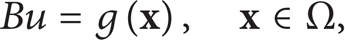
where x = (x,y) Δ is a second-order linear Laplace operator; α(x), β(x), γ(x), f(x), and g(x) are given functions; and B is the boundary differential operator.

Convert (3) into a Possion-type equation, moving the items other than the second-order partial derivative item to the right end of the equation:

$\Delta u=H\left(\mathbf{x},u,u_x,u_y\right)=-\alpha \left(\mathbf{x}\right)\frac{\partial u}{\partial x}-\beta \left(\mathbf{x}\right)\frac{\partial u}{\partial y}-\gamma \left(\mathbf{x}\right)u+f\left(\mathbf{x}\right).$

(5)

Utilize the interpolation of radial basis function ϕ, and H(x,u,u _x ,u _y ) can be approximately received:

$\begin{array}{c}\Delta u=H\left(\mathbf{x},u,u_x,u_y\right)\cong {{\displaystyle \sum }}_{i=\mathrm{1}}^n{a}_i\varphi \left(r_i\right),\end{array}$

(6)

where $r_i=\parallel \mathbf{x}-{\mathbf{x}}_i\parallel$ ${\{{\mathbf{x}}_i\}}_{i=\mathrm{1}}^{i=n}$ are the interpolation points; a_i is unknown coefficient; and ϕ is a unary function from R⁺ →R.

From (6),

$\begin{array}{c}u\left(\mathbf{x}\right)\cong {{\displaystyle \sum }}_{i=\mathrm{1}}^n{a}_i\Phi \left(r_i\right),\end{array}$

(7)

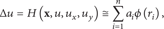
where ΔΦ = ϕ, ϕ is a given function, selected as function MQ in the MPS and expressed as $\sqrt{r^{\mathrm{2}}+c^{\mathrm{2}}}$ , where r is Euclidean distance, $r_j=\sqrt{{(x-x_j)}^{\mathrm{2}}+{(y-y_j)}^{\mathrm{2}}}$ , and c is a parameter with no theoretical recommended values until now. This paper chooses 8 times of mean particle spacing as c by trial.

So Φ can be obtained by repeated integral of ϕ [12, 13]. If function MQ is selected as the radial basis function, its special solution (MAPS) is expressed as follows:

$\Phi =\frac{\mathrm{1}}{\mathrm{9}}\left(\mathrm{4}{c}^{\mathrm{2}}+r^{\mathrm{2}}\right)\sqrt{r^{\mathrm{2}}+c^{\mathrm{2}}}-\frac{c^{\mathrm{3}}}{\mathrm{3}}\ln \left(c+\sqrt{r^{\mathrm{2}}+c^{\mathrm{2}}}\right).$

(8)

Partial derivative of Φ is

$\frac{\partial \Phi }{\partial x_k}=\frac{\mathrm{1}}{\mathrm{3}}\left[c^{\mathrm{2}}+\varphi \left(r^{\mathrm{2}}\right)-\frac{c^{\mathrm{3}}}{\varphi \left(r\right)}\right]\frac{x_k-x_k^j}{\varphi \left(r\right)},$

(9)

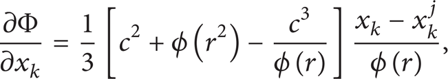
where x_k means the kth coordination direction.

From (3) and (6),

$\begin{array}{c}{{\displaystyle \sum }}_{i=\mathrm{1}}^n{a}_i\varphi \left(r_i\right)\cong -\alpha \left(\mathbf{x}\right)\frac{\partial u}{\partial x}-\beta \left(\mathbf{x}\right)\frac{\partial u}{\partial y}-\gamma \left(\mathbf{x}\right)u+f\left(\mathbf{x}\right).\end{array}$

(10)

Consider that the items on the right has this relation, $\partial u/\partial x\approx {\sum }_{i=\mathrm{1}}^n{a}_i(\partial \Phi /\partial x)(r_i)$ , $\partial u/\partial y\approx {\sum }_{i=\mathrm{1}}^n{a}_i(\partial \Phi /\partial y)(r_i)$ , so (10) can be simplified as

${{\displaystyle \sum }}_{i=\mathrm{1}}^n{a}_i\Psi \left(r_i\right)\cong f\left(\mathbf{x}\right),\hspace{1em}\mathbf{x}\in \Omega ,$

(11)

where

$\Psi \left(r_i\right)=\varphi \left(r_i\right)+\alpha \left(\mathbf{x}\right)\frac{\partial \Phi }{\partial x}\left(r_i\right)+\beta \left(\mathbf{x}\right)\frac{\partial \Phi }{\partial y}\left(r_i\right)-\gamma \left(\mathbf{x}\right)\Phi \left(r_i\right).$

(12)

In a similar way, the boundary condition is transformed as

${\displaystyle \sum }_{i=\mathrm{1}}^n{a}_{i}B\Phi \left(r_i\right)=g\left(\mathbf{x}\right),\hspace{1em}\mathbf{x}\in \partial \Omega .$

(13)

Finally, select two point sets, one for boundary point, while the other group for the interior points in the computational domain. Coefficients {a _i }_{i = 1} ⁿ in (11) and (13) can be derived by the collocation method, and thus approximate special solution $\widehat{u}$ can be worked out.

5. Localization of MAPS (LMAPS)

Because the MAPS is a meshless method based on the global RBFs, so the coefficient matrix is always a full matrix, sometimes even more ill-conditioned, which brings a lot of difficulty in solving large scale problem [14].

Inspired by the finite element method, as for the MAPS method, solve low order linear system of equations in the subdomain to obtain the linear combination coefficient. Then promote it to the global sparse matrix. This way avoids the problem of ill-conditioned matrix and guarantees the computational efficiency and accuracy [15, 16].

Presume for all x _p ∈Ω, and choose n_s nearest points (including the point itself) to build a support region Ω _p . Based on method of special solution, approximate solution of u(x _p ) can be expressed as linear combination as follows:

$u\left({\mathbf{x}}_p\right)\cong {{\displaystyle \sum }}_{i=\mathrm{1}}^{ns}{a}_i\Phi \left(\parallel {\mathbf{x}}_p-{\mathbf{x}}_j\parallel \right),$

(14)

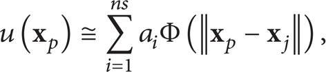
where {a _i }_{i = 1} ^ns is the required coefficient, all the problems focus on how to solve a_i, so a brief introduction is followed.

Ant point in the domain meets the relationship above, which can be written in matrix form:

$\left(\begin{array}{c}u\left({\mathbf{x}}_{\mathrm{1}}\right)\\ u\left({\mathbf{x}}_{\mathrm{2}}\right)\\ \cdots \\ u\left({\mathbf{x}}_N\right)\end{array}\right)\hspace{1em}=\left(\begin{array}{cccc}{\Phi }_{\mathrm{1}}\left({\mathbf{x}}_{\mathrm{1}}\right)& {\Phi }_{\mathrm{1}}\left({\mathbf{x}}_{\mathrm{2}}\right)& \cdots & {\Phi }_{\mathrm{1}}\left({\mathbf{x}}_{ns}\right)\\ {\Phi }_{\mathrm{2}}\left({\mathbf{x}}_{\mathrm{1}}\right)& {\Phi }_{\mathrm{2}}\left({\mathbf{x}}_{\mathrm{2}}\right)& \cdots & {\Phi }_{\mathrm{2}}\left({\mathbf{x}}_{ns}\right)\\ \cdots & \cdots & \cdots & \cdots \\ {\Phi }_{ns}\left({\mathbf{x}}_{\mathrm{1}}\right)& {\Phi }_{ns}\left({\mathbf{x}}_{\mathrm{2}}\right)& \cdots & {\Phi }_{ns}\left({\mathbf{x}}_{ns}\right)\end{array}\right)\left(\begin{array}{c}{a}_{\mathrm{1}}\\ a_{\mathrm{2}}\\ \cdots \\ a_{ns}\end{array}\right),$

(15)

where ${\Phi }_i(\mathbf{x})=\Phi (\parallel \mathbf{x}-{\mathbf{x}}_i\parallel )$ .

Define the coefficient matrix above as 𝚽 _ns ; namely,

${\mathbf{a}}_{ns}={𝚽}_{ns}^{-\mathrm{1}}{\mathbf{u}}_{ns}.$

(16)

Substitute (16) into (14),

$\begin{array}{c}u\left({\mathbf{x}}_p\right)\cong {{\displaystyle \sum }}_{i=\mathrm{1}}^{ns}{a}_i\Phi \left(\parallel {\mathbf{x}}_p-{\mathbf{x}}_j\parallel \right)={𝚽}_{ns}\left({\mathbf{x}}_p\right){\mathbf{a}}_{ns}={𝚽}_{ns}\left({\mathbf{x}}_p\right){𝚽}_{ns}^{-\mathrm{1}}{\mathbf{u}}_{ns}={𝚿}_{ns}\left({\mathbf{x}}_p\right){\mathbf{u}}_{ns}.\end{array}$

(17)

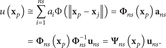
The formula above has simplified the solution of a_i into the calculation of known function Φ. Therefore, solving the vector {u _i }_{i = 1} ^ns turns easy.

Approximate function of partial differential equation like (11) can be written as

$f\left({\mathbf{x}}_p\right)={\mathbf{\Theta }}_{ns}{\mathbf{a}}_{ns}={\mathbf{\Theta }}_{ns}\left({\mathbf{x}}_p\right){𝚽}_{ns}^{-\mathrm{1}}{\mathbf{u}}_{ns},$

(18)

where

${\Theta }_{pj}=\varphi \left(\parallel {\mathbf{x}}_p-{\mathbf{x}}_j\parallel \right)+\alpha \left({\mathbf{x}}_p\right){\Phi }_x\left(\parallel {\mathbf{x}}_p-{\mathbf{x}}_j\parallel \right)\hspace{1em}+\beta \left({\mathbf{x}}_p\right){\Phi }_y\left(\parallel {\mathbf{x}}_p-{\mathbf{x}}_j\parallel \right)+\gamma \left({\mathbf{x}}_p\right)\Phi \left(\parallel {\mathbf{x}}_p-{\mathbf{x}}_j\parallel \right),\hspace{1em}\hspace{1em}\hspace{1em}\hspace{1em}\hspace{1em}\hspace{1em}\hspace{1em}\hspace{1em}\hspace{1em}\hspace{1em}\hspace{1em}\hspace{1em}\hspace{1em}\hspace{1em}j=\mathrm{1,2},\dots ,n_s.$

(19)

Now define 𝚿 _ns (x _p ) = Θ _ns (x _p )𝚽 _ns ⁻¹ = [C₁,C₂,…, C _ns ], so (18) can be simplified as

${𝚿}_{ns}\left({\mathbf{x}}_p\right){\mathbf{u}}_{ns}=f\left({\mathbf{x}}_p\right),\hspace{1em}{\mathbf{x}}_p\in {\Omega }_p.$

(20)

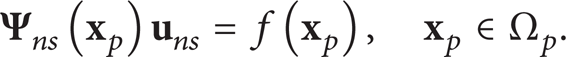
Referring to the prolongation method described in [13], add n-n _s zero element in the suitable position of vector 𝚿 _ns (x _p ) to form a sparse matrix. The process is similar as formation of overall stiffness matrix in FEM.

Similar to the above steps operating on (3), scatter (4) as follows:

$g\left({\mathbf{x}}_i\right)=B{𝚽}_n\left({\mathbf{x}}_i\right){𝚽}_n^{-\mathrm{1}}\left({\mathbf{x}}_i\right){\mathbf{u}}_n={\phi }_n\left({\mathbf{x}}_i\right){\mathbf{u}}_n.$

(21)

Finally, unite formulae (20) and (21) to get the n-order sparse linear equations as follows:

$\left[\begin{array}{c}{\Psi }_n\left({\mathbf{x}}_{\mathrm{1}}\right)\\ \cdots \\ {\Psi }_n\left({\mathbf{x}}_{ni}\right)\\ {\phi }_n\left({\mathbf{x}}_{ni+\mathrm{1}}\right)\\ \cdots \\ {\phi }_n\left({\mathbf{x}}_n\right)\end{array}\right]\left[\begin{array}{c}u\left({\mathbf{x}}_{\mathrm{1}}\right)\\ \cdots \\ u\left({\mathbf{x}}_{ni}\right)\\ u\left({\mathbf{x}}_{ni+\mathrm{1}}\right)\\ \cdots \\ u\left({\mathbf{x}}_n\right)\end{array}\right]=\left[\begin{array}{c}f\left({\mathbf{x}}_{\mathrm{1}}\right)\\ \cdots \\ f\left({\mathbf{x}}_{ni}\right)\\ f\left({\mathbf{x}}_{ni+\mathrm{1}}\right)\\ \cdots \\ f\left({\mathbf{x}}_n\right)\end{array}\right].$

(22)

By solving (22), the approximate values of any given point of function u can be obtained.

6. Discretization of N-S Equation Set

Generally speaking, N-S equations of incompressible unsteady fluid are written as

Continuity equation:

$\nabla ·\mathbf{u}=\mathrm{0}.$

(23)

Momentum equation:

$\frac{\partial \mathbf{u}}{\partial t}+\mathbf{u}·\nabla \mathbf{u}=-\nabla p+\frac{\mathrm{1}}{\mathrm{Re}}\Delta \mathbf{u}\mathbf{,}$

(24)

where p is fluid pressure; u is the flow velocity; and Re is the flowing Reynolds number.

It can be seen that the velocity u and pressure p in the above equation are coupled with each other, while the pressure p has no independent equations. Therefore, choose projection method to separate the pressure item for solution.

Projection method, also known as fractional method, is proposed by Chorin and Temam [17] in 1968. The specific steps are as follows.

Step 1. Compared to (24), use explicit difference method to calculate the temporary velocity u^*, in which u ⁿ is the calculated velocity in the nth step:

$\frac{\partial {\mathbf{u}}^{*}}{\partial t}=\frac{{\mathbf{u}}^{*}-{\mathbf{u}}^n}{\Delta t}=-{\mathbf{u}}^{*}·\nabla {\mathbf{u}}^{*}+\frac{\mathrm{1}}{\mathrm{Re}}\Delta \mathbf{u}\mathbf{.}$

(25)

Known from Step 1, temporary velocity needs to meet

$\frac{{\mathbf{u}}^{n+\mathrm{1}}-{\mathbf{u}}^{*}}{\Delta t}+\nabla p^{n+\mathrm{1}}=\mathrm{0}.$

(26)

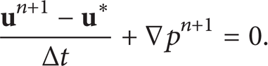
Taking the divergence of the above formula, combining the formula (23),

$\Delta p^{n+\mathrm{1}}=\frac{\nabla {\mathbf{u}}^{*}}{\Delta t}.$

(27)

Formula (27) is a typical Possion-type equation. It can be easily solved by the application of LMAPS method in the previous part.

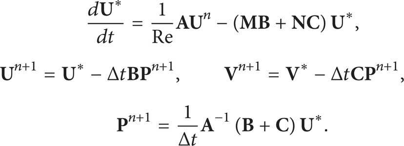
Step 2. For two-dimensional flow problems, three formulas above are dispersed as follows:

$\begin{array}{c}\frac{{\mathbf{u}}_i^{*}-{\mathbf{u}}_i^n}{\Delta t}=\frac{\mathrm{1}}{\mathrm{Re}}{{\displaystyle \sum }}_{n=\mathrm{1}}^{ns}{a}_{ij}{\mathbf{u}}_j^n-\left(u_i^n{{\displaystyle \sum }}_{j=\mathrm{1}}^{ns}{b}_{ij}{\mathbf{u}}_j^n+v_i^n{{\displaystyle \sum }}_{j=\mathrm{1}}^{ns}{c}_{ij}{\mathbf{u}}_j^n\right),\\ u_i^{n+\mathrm{1}}=u_i^{*}-\Delta t{{\displaystyle \sum }}_{j=\mathrm{1}}^{ns}{b}_{ij}{p}_i^n,\hspace{1em}\hspace{1em}{v}_i^{n+\mathrm{1}}=v_i^{*}-\Delta t{{\displaystyle \sum }}_{j=\mathrm{1}}^{ns}{c}_{ij}{p}_i^n,\\ \Delta p_i^{n+\mathrm{1}}=\frac{\mathrm{1}}{\Delta t}\left({{\displaystyle \sum }}_{j=\mathrm{1}}^{ns}{b}_{ij}{\mathbf{u}}_j^{*}+{{\displaystyle \sum }}_{j=\mathrm{1}}^{ns}{c}_{ij}{\mathbf{u}}_j^{*}\right),\end{array}$

(28)

where n represents the time step of solution; x_i (i = 1, 2,…, n _s ) is the node within the support region; and a _ij ,b _ij , and c _ij are the unknown coefficients, which can be solved by the method described in the previous section.

Step 3. Form the whole sparse matrix through the assembly of formula above,

$\begin{array}{c}\frac{d{\mathbf{U}}^{*}}{dt}=\frac{\mathrm{1}}{\mathrm{Re}}\mathbf{A}{\mathbf{U}}^n-\left(\mathbf{M}\mathbf{B}+\mathbf{N}\mathbf{C}\right){\mathbf{U}}^{*},\\ {\mathbf{U}}^{n+\mathrm{1}}={\mathbf{U}}^{*}-\Delta t\mathbf{B}{\mathbf{P}}^{n+\mathrm{1}},\hspace{1em}\hspace{1em}{\mathbf{V}}^{n+\mathrm{1}}={\mathbf{V}}^{*}-\Delta t\mathbf{C}{\mathbf{P}}^{n+\mathrm{1}},\\ {\mathbf{P}}^{n+\mathrm{1}}=\frac{\mathrm{1}}{\Delta t}{\mathbf{A}}^{-\mathrm{1}}\left(\mathbf{B}+\mathbf{C}\right){\mathbf{U}}^{*}.\end{array}$

(29)

Get the results of each time step in accordance with this order until the solution is completely done.

7. Wave Generation by Momentum Source

Wave generation technology for numerical wave flume can generally be divided into two types. First, the physical wave generation technology; that is to simulate the reciprocating motion of laboratory push-wave plate to impose forced displacement on water bodies to form waves. In the mathematical model, control signal of the numerical push-wave plate can be directly obtained from the physical wave machine. This technology is more traditional and more mature, but the incident wave will pass through the wave machine after the reflection by buildings, generating secondary reflection at the push-wave plate, resulting in the gradual accumulation of energy. It has ignorable impact on the experimental results. The results of the active wave absorption technology currently adopted are not ideal enough. Another technique is the momentum source wave generation technology, a purely numerical approach, which is a mandatory assignment of velocity of nodes in computational domain for the velocity of water particles in target wave, using a series of damping absorbing programs to eliminate reflected wave, thus eliminating the impact of secondary reflection at a great extent.

Israeli and Orszag [18] proposed the concept of source wave generation and subsequently carried out in-depth research. Currently, the source wave generation technology has been widely applied to build the numerical wave flume based on finite element method (FEM), finite volume method (VOF), and other methods. But the combination of source wave generation technology and the LMAPS method has no corresponding literature report at home and abroad until now. This paper proposed the source wave generation technology, suitable for the LMAPS method, to generate various kinds of waves as needed, which makes LMAPS method can be widely used.

In the momentum source wave technology, source function is derived firstly based on the governing equations. The meaning of source function can be seen as the momentum, changing periodically over time applied on fluid in wave zone; thus the numerical wave can be simulated. In addition, the reflection and the secondary reflection at the boundary cannot be ignored.

Based on the thought of analytical relaxation, this paper uses wave generation and wave absorption method to produce reasonable waves, which handles the wave reflection effects. As for the free surface flow simulated in this paper, modify the momentum equation (24) into the following form:

$\frac{\partial \mathbf{u}}{\partial t}+\mathbf{u}·\nabla \mathbf{u}=-\nabla p+\frac{\mathrm{1}}{\mathrm{Re}}\Delta \mathbf{u}+\mathbf{W}+\mathbf{I}\mathbf{,}$

(30)

where W is the gravity of fluid and I is the additional momentum source. Figure 1 shows the picture of wave maker principal.

Figure 1:

Schematic layout of numerical wave flume.

By the role of additional momentum source, assume that particle in wave generation area moves as follows:

$u_m=C{u}_{\mathrm{1}},\hspace{1em}\hspace{1em}{v}_m=C{v}_{\mathrm{1}},\hspace{1em}\hspace{1em}{p}_m=C{p}_{\mathrm{1}}.$

(31)

While particle in the damping layer moves as follows:

$u_m=C{u}_c+\left(\mathrm{1}-C\right)u_{\mathrm{1}},\hspace{1em}\hspace{1em}{v}_m=C{v}_c+\left(\mathrm{1}-C\right)v_{\mathrm{1}},\begin{array}{c}{p}_m=C{p}_c+\left(\mathrm{1}-C\right)p_{\mathrm{1}}.\end{array}$

(32)

In these formulae, C = C(x) is a spatial distribution function, which expresses the general shape of the flow velocity distribution with height. It can be linear function or other nonlinear functions. Take the above equation into the governing equation to get the two types of equations.

In the wave zone, the additional momentum source can be expressed as

$I_x=\left(\mathrm{1}-C\right)\left(\frac{\partial p_c}{\partial x}-\rho \frac{u_c}{\Delta t}\right)+\rho \left(\mathrm{1}-C^{\mathrm{2}}\right)\left(u_c\frac{\partial u_c}{\partial x}+v_c\frac{\partial u_c}{\partial y}\right),\begin{array}{c}{I}_y=\left(\mathrm{1}-C\right)\left(\frac{\partial p_c}{\partial y}-\rho \frac{v_c}{\Delta t}\right)\hspace{1em}+\rho \left(\mathrm{1}-C^{\mathrm{2}}\right)\left(u_c\frac{\partial v_c}{\partial x}+v_c\frac{\partial v_c}{\partial y}\right)-\rho g.\end{array}$

(33)

In the damping region, the additional momentum source can be expressed as

$\begin{array}{c}{I}_x=\frac{\rho }{\Delta t}\left(C-\mathrm{1}\right)\left(u_c-u_{\mathrm{1}}\right)+\rho \left(\mathrm{1}-C\right)\hspace{1em}\times \left(\frac{\mathrm{1}}{\rho }\frac{\partial p_c}{\partial x}+\frac{\partial u_c}{\partial t}+u_{\mathrm{1}}\frac{\partial u_{\mathrm{1}}}{\partial x}+v_{\mathrm{1}}\frac{\partial u_{\mathrm{1}}}{\partial y}\right)\hspace{1em}-\rho \{\left(C^{\mathrm{2}}-\mathrm{1}\right)\left(u_c\frac{\partial u_c}{\partial x}+v_c\frac{\partial u_c}{\partial y}\right)\hspace{1em}\hspace{1em}\hspace{1em}+\left(\mathrm{1}-C^{\mathrm{2}}\right)\left(u_{\mathrm{1}}\frac{\partial u_{\mathrm{1}}}{\partial x}+v_{\mathrm{1}}\frac{\partial u_{\mathrm{1}}}{\partial y}\right)+C\left(\mathrm{1}-C\right)\hspace{1em}\hspace{1em}\hspace{1em}\times \left[\left(u_c\frac{\partial u_{\mathrm{1}}}{\partial x}+v_c\frac{\partial u_{\mathrm{1}}}{\partial y}\right)+\left(u_{\mathrm{1}}\frac{\partial u_c}{\partial x}+v_{\mathrm{1}}\frac{\partial u_c}{\partial y}\right)\right]\phantom{\left(u_c\frac{\partial v_c}{\partial x}+v_c\frac{\partial v_c}{\partial y}\right)}\},\\ I_y=\frac{\rho }{\Delta t}\left(C-\mathrm{1}\right)\left(v_c-v_{\mathrm{1}}\right)+\rho \left(\mathrm{1}-C\right)\hspace{1em}\times \left(\frac{\mathrm{1}}{\rho }\frac{\partial p_c}{\partial y}+\frac{\partial v_c}{\partial t}+u_{\mathrm{1}}\frac{\partial v_{\mathrm{1}}}{\partial x}+v_{\mathrm{1}}\frac{\partial v_{\mathrm{1}}}{\partial y}-g\right)\hspace{1em}-\rho \{\left(C^{\mathrm{2}}-\mathrm{1}\right)\left(u_c\frac{\partial v_c}{\partial x}+v_c\frac{\partial v_c}{\partial y}\right)\hspace{1em}\hspace{1em}\hspace{1em}+\left(\mathrm{1}-C^{\mathrm{2}}\right)\left(u_{\mathrm{1}}\frac{\partial v_{\mathrm{1}}}{\partial x}+v_{\mathrm{1}}\frac{\partial v_{\mathrm{1}}}{\partial y}\right)+C\left(\mathrm{1}-C\right)\hspace{1em}\hspace{1em}\hspace{1em}\times \left[\left(u_c\frac{\partial v_{\mathrm{1}}}{\partial x}+v_c\frac{\partial v_{\mathrm{1}}}{\partial y}\right)+\left(u_{\mathrm{1}}\frac{\partial v_c}{\partial x}+v_{\mathrm{1}}\frac{\partial v_c}{\partial y}\right)\right]\phantom{\left(u_c\frac{\partial v_c}{\partial x}+v_c\frac{\partial v_c}{\partial y}\right)}\}.\end{array}$

(34)

8. Waves Climbing Verification

Accurate reproduction of waves climbing process is the premise of accurate study of wave overtopping. To verify the reliability of wave process simulation, based on the LMAPS method innovated by this paper, we quote the physical model test data conducted by Li et al. [19]. Describe the validity of the LMAPS model by comparing wave surface elevation on corresponding position both in the physical model and the mathematical model.

Gradient of the sloping dike used in the experiments is 1: 6, water depth at the toe is 0.7 m, wave height is 0.16 m, and trial wave period is 2's. Monitoring point WG1 is for measuring the wave height before climbing. Monitoring points WG2 and WG3 are located on the slope surface. The horizontal distance from the foot of the slope to these two points is 1.02 m and 2.81 m, respectively, shown in Figure 2. Figure 3 shows the wave surface's changing process over time in the monitoring points of WG2 and WG3. Solid line is the numerical simulation results by the LMAPS method, of while hollow circle is the physical model results done by Li et al. It can be seen from the figure that these calculation results agree well with the physical model results. Wave height, wave phase, and wave skewness all get better reflect.

Figure 2:

Test layout of waves climbing verification.

Figure 3:

Verification of waves climbing process.

9. Overtopping Calculation under Regular Waves

This paper employs the LMAPS method to solve N-S equations, in order to simulate the wave climbing and broken on sloping dike and other physical phenomena. It uses Shepard filter [20] to deal with nonphysical pressure shocks. Hu et al. [6] selected 20 test conditions from Saville's [1] physical model, analyzed, and summarized the formula of dimensionless overtopping:

$Q=\frac{q}{H_{\mathrm{0}}\sqrt{g{H}_{\mathrm{0}}}},$

(35)

where q is the average overtopping unit width (m³/(m·s)) and H0 is wave height for deep water, taken as 1 m in this test.

For the test conditions chosen by Hu et al., this paper uses the LMAPS method to establish particle model (parameters in Table 1). Figure 4 shows the test arrangement layout of overtopping on sloping dike in which d_t means the depth of the test flume; d_s means the water depth at the toe of the sloping dike; R _c is the ultrahigh of the sloping dike; and T _s is the wave period. The sloping dike is arranged on the top of a 1: 10 gentle slope. In Run 1∼Run 16, the gradient of the sloping dike is 1: 3, in Run 17∼Run 20, and it is 1: 1.5. Particle counter is set as 0.5 m away from the dike frontier. Calculate overtopping by monitoring, the total number of water particles right of the counter. The initial particle spacing in calculation is set as 0.005 m. Arrange four rows of particles as a fixed boundary. Total duration of the simulation is 40's.

Table 1:

Test condition parameters and particle number of regular wave overtopping [21].

m	dt (m)	ds (m)	R c (m)	H t (m)	T (s)	Particle number
Run 1	3.00	0.75	0.50	0.95	4.73	64656
Run 2	3.00	0.75	1.00	0.95	4.73	65048
Run 3	3.00	1.50	0.50	0.95	4.73	61747
Run 4	3.00	1.50	1.00	0.95	4.73	62155
Run 5	4.00	2.00	0.67	0.99	6.55	99154
Run 6	4.00	0.75	0.50	1.08	7.98	130392
Run 7	4.50	0.75	1.00	1.06	7.98	151554
Run 8	4.00	0.75	1.50	1.08	7.98	131434
Run 9	4.00	1.50	0.50	1.08	7.98	127045
Run 10	4.00	1.50	1.00	1.08	7.98	127305
Run 11	4.00	1.50	1.50	1.08	7.98	127767
Run 12	6.00	1.00	0.67	1.20	12.80	275857
Run 13	6.00	2.00	0.67	1.20	12.80	269804
Run 14	6.00	2.00	1.33	1.20	12.80	270724
Run 15	6.00	2.00	2.00	1.20	12.80	271548
Run 16	6.00	2.00	2.67	1.20	12.80	272425
Run 17	4.92	0.75	0.50	1.04	7.98	157508
Run 18	4.92	0.75	1.50	1.04	7.98	157947
Run 19	4.17	0.00	0.50	1.07	7.98	129441
Run 20	4.17	0.00	1.00	1.07	7.98	129699

Figure 4:

Test arrangement layout of regular wave overtopping.

Similar to physical model test, the first few waves are more unstable during wave generation process. So this paper chooses the 4th to 6th wave action process to get the average overtopping and compare the overtopping values with that of Saville [1], Kobayashi and Wurjanto [5], and Hu et al. [6], shown in Figure 5 in detail. It can be seen from Figure 5 that the numerical results by the LMAPS method are more consistent with the physical model test results. Compared to the physical test values, the average error is 22.0%, while for Kobayashi and Wurjanto [5], the average error is about 50.6%, for Hu et al., and the average error is about 34.5%, meaning that the LMAPS is methods more advantaged after comparison.

Figure 5:

Results comparison of regular wave overtopping.

10. Impact of Different Types of Wave Walls on Wave Overtopping

This paper refers to the physical model tests by Saville and selects six kinds of wave walls for overtopping simulation (vertical wave wall, 1/4 arc wave wall, reversed-arc wave wall, smooth surface wave wall with 1: 3 slope ratio, smooth surface wave wall with 1: 1.5 slope ratio, and stepped surface wave wall with 1: 1.5 slope ratio, shown in Figure 6). Arrangements adopted here are similar with the previous section, including a 1: 10 gentle slope, with a wave wall on the top of it. Water depth in front of the gentle slope d _t = 8.99 m, water depth at the toe of the wave wall d _s = 1.37 m, ultrahigh of the wave wall R _c = 0.91 m, regular wave height H₀ = 1.83 m, and period T = 6.40's.

Figure 6:

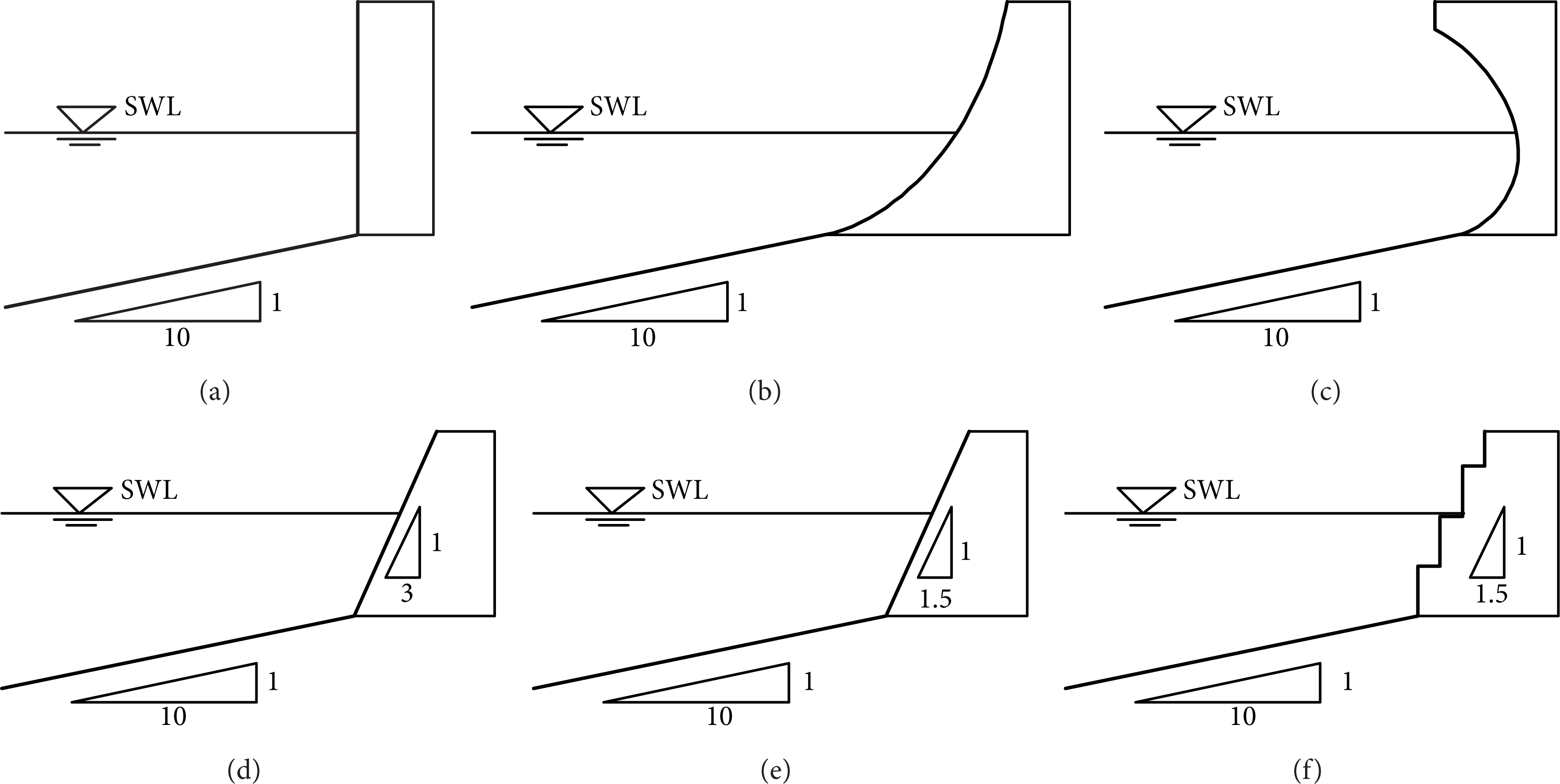
Scheme illustrations of six different structural forms of wave walls.

Figure 7 shows the wave feature when waves shock instantaneously on the six kinds of wave walls. Contours with different colors represent the absolute magnitude of the velocity of water particles. After shocking on the vertical wall (a), wave's velocity magnitude and direction change sharply in a very short time. Part of the water fly into the air, forming wave overtopping. Wave action process on 1/4 arc wave wall (b) and reversed-arc wave wall (c) are relatively more relaxed. Arc surface of the 1/4 arc wave wall leads waves to vertical upward flow: part of the water bodies falls back into the sea under gravity, and the other part gets over the crown, forming overtopping. As to the reversed-arc wave wall, most water bodies fall back again into the sea, and only a small part of it can climb over the top, so the overtopping volume of this type is the smallest between the six types. For (d), (e), and (f), three conditions, with the terrain slope being larger, wave steepness also becomes larger rapidly, and wave crest bends forward and also wave breaks. Broken wave climb along the wave wall up, eventually cross over it. Overall, the LMAPS method can relatively accurately simulate interaction results between waves and different types of wave walls.

Figure 7:

Wave feature on the overtopping moment with six kinds of wave walls.

Compare the calculated dimensionless overtopping in this paper with Saville's physical model results, shown in Figure 8. Both the data are very consistent, and the average error is about 6.2%. Compared with each working conditions, it can be found that the overtopping on sloping dike increases with the slowdown of gradient; the stepped surface can further hinder fluid climbing and help reduce overtopping; reversed-arc wave wall has the most significant force on wave overtopping control.

Figure 8:

Overtopping results comparison of different structural forms of wave walls.

11. Conclusions and Outlook

Based on the LMAPS method, this paper proposes source wave generation and wave absorption technology that is suitable for this particle algorithm and establishes a two-dimensional numerical wave flume. Afterwards, climbing and overtopping process under regular waves on particular sloping dike by 20 groups of different working conditions are simulated. The calculated results are compared with the experimental results and the results obtained by previous researchers. The average error of the average overtopping calculated by the LMAPS method is approximately 22.0% compared with the experimental values, less than that of Kobayashi and Wurjanto [5] and Hu et al. [6], indicating the stability and reliability of LMAPS.

Finally, numerical calculation results for overtopping under regular waves on six different structural forms of wave walls accurately describe the morphological changes when waves are interacted with different wave walls. The calculated average overtopping is within the control of 6.2% compared with the experimental value, and the overtopping on reversed-arc wave wall is significantly less than other types of wave walls.

Conflict of Interests

The authors declare that there is no conflict of interests regarding the publication of this paper.