Sage Journals: Discover world-class research

Abstract

Fish are very efficient swimmers. In this paper, we studied a two degree-of-freedom (DOF) propeller that mimic fish caudal fin like locomotion. Kinematics modelling and hydrodynamic CFD analyses of the two DOF propellers were conducted. According to the CFD simulation, we show that negative power was generated within the flapping cycle, and wake flow at different instant was demonstrated. Based on the dynamic model, we compared the thrust efficiency under different stiffness control method. The results show that the thrust efficiency was enhanced under moderate stiffness control strategy.

1. Introduction

Fish are very efficient swimmers. They have a number of swimming modes that are worth considering for emulation, but the locomotion that has long attracted the attentions of both biologists [1, 2] and engineers [3, 4] is the body/caudal fin undulatory kinematics. Many papers have addressed the live undulatory locomotion of fish over the past few years. But studying how fish generate the external fluid force to swim has proven to be difficult and is limited in the ability of controlling for parameters in a precise and repeatable manner. There still exist several important questions about kinematic effects on the hydrodynamics. In many previous studies of fish swimming, the fish undulatory body and flapping caudal fin kinematics are treated together as a derivable mathematical wave [2]. Nevertheless, recent biological findings indicate that the caudal fin undergoes complex kinematics independent of the body in lots of bony fish because of their stiffness. Both body undulation and caudal fin flapping play essential roles while a fish is swimming [5 –13]. How does the flexure stiffness affect the hydrodynamics of the fish swimming? To what extent does the stiffness contribute to the overall swimming performance? In addition, how is the wake flow generated as a function of the stiffness of the flapping caudal fin? The questions presented above are certainly not the only possible ones worth discussion but can serve as a starting point for thinking.

The lateral muscles of fish shorten and lengthen alternatively on either side. When the shortening muscles exert a contraction force, they do positive work. In other parts the muscles may be stretched while they exert a contracting force; there they do negative work. A fish's swimming strategy may involve an alternative contraction of all the lateral muscles on either side of the body. Fish swim with lateral body undulation waves running from head to tail; however, these waves run more slowly than the waves of muscle activation causing them, which reflect the effect of the reactive forces from the water [14, 15]. The phase relationship between the strain (muscle length change) cycle and the active period (when force is generated) determines the work output of the muscle. The posterior muscle of some fish, such as trout, saithe, and scup, generates negative power while swimming. In addition, biologists show that the swimming fish can use environmental vortices, which is likely to reduce the cost of locomotion [16]. The fish extracts energy and generates sufficient thrust to overcome its drag. Namely, energy extraction is achieved when the flexural stiffness of the swimming fish body interacted with water moderately and resonated in a natural mode with oncoming Karman Street eddies [17].

In this paper, we aim to investigate the stiffness effect on the unsteady fish-like propulsion by using simulation approach. More specifically, we implemented a bioinspired two degree-of-freedom propeller and programmed it with different flexure stiffness. Understanding how the stiffness of a propeller affects its thrust performance requires knowledge and data of the hydrodynamics. Simulation was implemented for obtaining quantitative torque, power, and wake flow of the propeller under dynamic condition. Based on the dynamic model, we compared the thrust efficiency of the propeller under different stiffness control methods.

2. Materials and Methods

2.1. Model and Parameters of Robotic Fish

In the 1970s, Lighthill proposed the function of fish body curve; he used a quadratic curve to match fish's body midline and the function is described as [18]

y (x, t) = (c_{1} x + c_{2} x^{2}) \sin (\frac{2 π}{λ} x + ω t),

(1)

where y is the distance between body midline and the x-axis of the model; c1 is linear coefficient of body curve; c2 is quadratic coefficient of body curve; λ is the wavelength described as λ = L_f/R; L_f is the length of the robotic fish; R is the number of body curve; ω is the frequency of body curve.

Two-joint robotic fish model consists of three parts: head and two joints. Figure 1 shows the two joints of the two-joint robotic fish model. The length of the model is L_f, the front 1/3 part of the model is head, the length of the first joint is L1, and that of the second joint is L2. In order to mimic live fish better, we need to optimize the length of robotic fish's body and tail. The principle of the optimization is to minimize the area S between the two joints and body midline of live fish. S can be described as

S = \sum_{i = 1}^{2} ‍ \int_{start_i}^{end_i} ‍ | f_{i} (x) - g_{i} (x) | d x,

(2)

where f_i(x) is the function of the joint of the robotic fish, g_i(x) is the function of the body midline of live fish, which is shown in Figure 1(c) with blue dot line. start_i is the start of the i joint and end_i is the end of the i joint. To mimic live fish, the parameters of the two joints should be set by the following conditions:

L₁ + L₂ + L_h = L_f;

S gets its minimum value.

Figure 1:

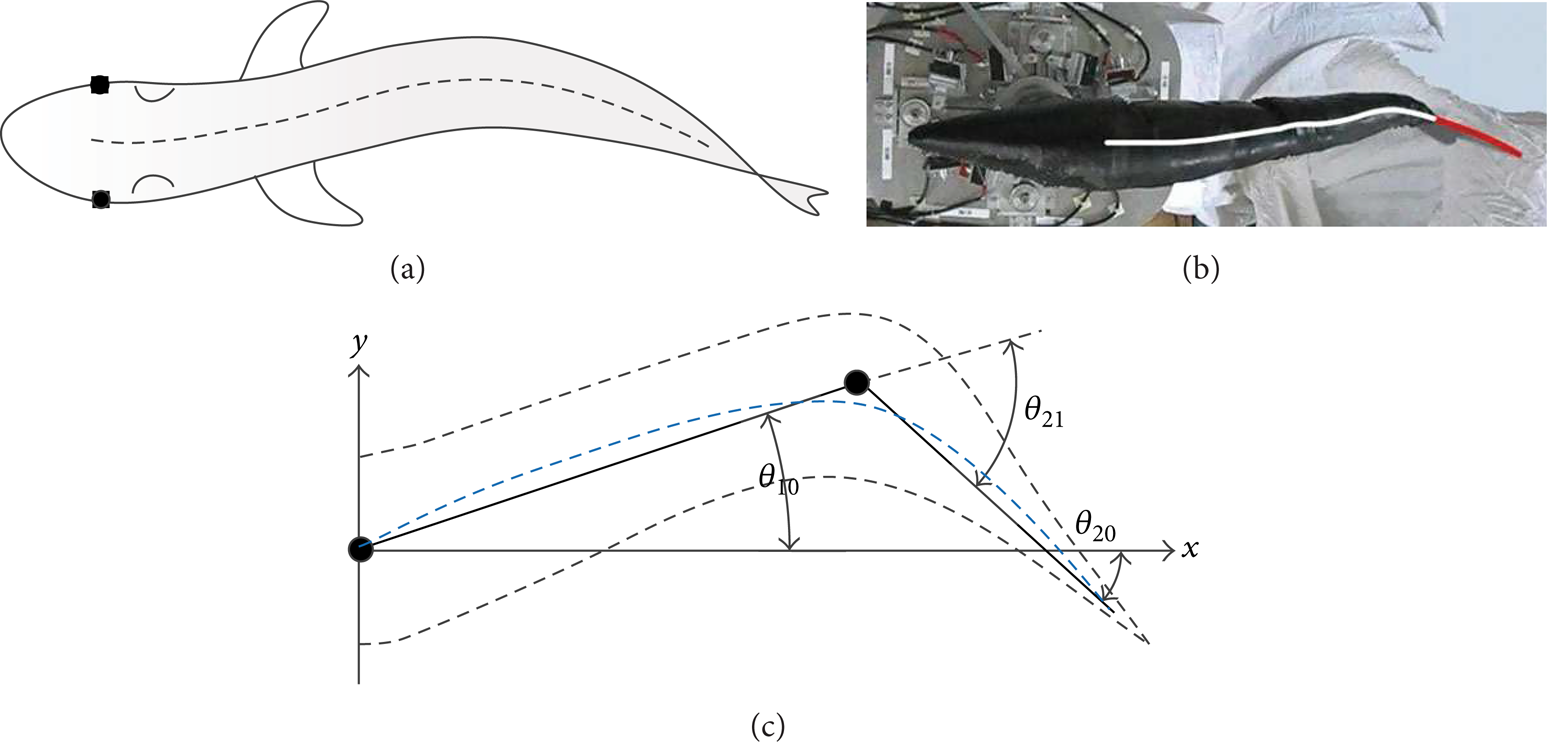
Fish model: (a) live fish outline; (b) robotic fish (Robotics Institute, Beihang University); (c) two-joint fish.

Wen et al. discussed the method to minimize S in [7].

Generally, joints of robotic fish are driven by motors; in order to mimic Lighthill's motion function, the angular function of each joint should be calculated. We can see from Lighthill's motion function that each point of the body midline is sinusoidal; we can get motion function of the two joints as shown in the following:

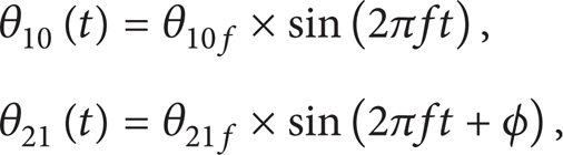
\begin{matrix} θ_{10} (t) = θ_{10 f} \times \sin (2 π f t), \\ θ_{21} (t) = θ_{21 f} \times \sin (2 π f t + ϕ), \end{matrix}

(3)

where θ₁₀(t) is the angle function between the first joint and x-axis, θ_10f is the amplitude of θ₁₀(t), θ₂₁(t) is the angle function between the second joint and the first joint, and θ_21f is the amplitude of θ₂₁(t). We can deduce from the motion function given by Lighthill that the phase difference of the two joints is

ϕ = \frac{2 π}{λ} Δ x .

(4)

The principle of determining θ_10f and θ_21f is that the end point of each joint coincides with the corresponding point of the body midline of live fish.

2.2. Dynamical Model

We use Lagrange-Euler method to analyze the dynamical model of the two-joint robotic fish.

Lagrange equation is shown as follows:

τ_{i} = \frac{d}{d t} [\frac{\partial L}{\partial {\dot{q}}_{i}}] - \frac{\partial L}{\partial q_{i}},

(5)

where τ_i is generalized force or torque of the system; q_i is system variable; ${\dot{q}}_{i}$ is the first derivative of the system variable; i is the number of system variables; L is Lagrange equation shown as follows:

L = K - P,

(6)

where K is kinetic energy of the system and P is the potential energy of the system. The potential energy of robotic fish system contains only gravitational potential energy; in our research the gravitational potential energy is constant as the robotic fish contains no vertical movement; therefore, the potential energy of the robotic system is zero; that is, P = 0.

Let L0 be the length of the head, let L1 be the length of the first joint, and let L2 be the length of the second joint.

We use concentrated forces F0, F1, and F2 to substitute the hydrodynamic force for simplification. There are three degrees of freedom in our system, the x-coordinate of the head X0, the angular between the head and the first joint θ₁₀, and the angular between the first joint and the second joint θ₂₁. We can get the dynamical model of the system as follows:

\begin{matrix} \frac{d}{d t} (\frac{\partial L}{\partial {\dot{θ}}_{10}}) - \frac{\partial L}{\partial θ_{10}} = Q_{1}, \\ \frac{d}{d t} (\frac{\partial L}{\partial {\dot{θ}}_{21}}) - \frac{\partial L}{\partial θ_{21}} = Q_{2}, \\ \frac{d}{d t} (\frac{\partial L}{\partial {\dot{X}}_{0}}) - \frac{\partial L}{\partial X_{0}} = Q_{3}, \end{matrix}

(7)

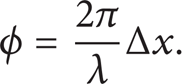
where Q1 is nonconservative force to generalized coordinate θ₁₀, Q2 is nonconservative force to generalized coordinate θ₂₁, and Q3 is nonconservative force to generalized coordinate X0. Liu talked about the formulas to calculate Q1 to Q3 which are described by the following equations [19]:

\begin{matrix} Q_{1} = {\vec{F}}_{1} \cdot (\begin{pmatrix} - L_{d 1} \sin θ_{10} \\ L_{d 1} \cos θ_{10} \end{pmatrix}) + {\vec{F}}_{2} \cdot (\begin{pmatrix} - L_{1} \sin θ_{10} - L_{d 2} \sin θ_{20} \\ L_{1} \cos θ_{10} + L_{d 2} \cos θ_{20} \end{pmatrix}) + M_{1}, \\ Q_{2} = {\vec{F}}_{2} \cdot (\begin{pmatrix} - L_{d 2} \sin θ_{20} \\ L_{d 2} \cos θ_{20} \end{pmatrix}) + M_{2}, \\ Q_{3} = {\vec{F}}_{0} \cdot (\begin{pmatrix} 1 \\ 0 \end{pmatrix}) + {\vec{F}}_{1} \cdot (\begin{pmatrix} 1 \\ 0 \end{pmatrix}) + {\vec{F}}_{2} \cdot (\begin{pmatrix} 1 \\ 0 \end{pmatrix}) . \end{matrix}

(8)

M₁ and M2 are the torques generated by the first and second joint; F0 is the resistance force of the fluid to the fish; F1 is the hydrodynamic force to the first joint; F2 is the hydrodynamic force to the second joint. Compared to resistant force, friction force on the body can be neglected. To simplify calculation, we use resistance force theory to calculate the hydrodynamic forces; therefore, the resistance force to the head can be calculated by the equation as follows:

F_{0} = \frac{1}{2} ρ C_{0} V_{0}^{2} A_{0},

(9)

where ρ is the density of the fluid, C0 is the resistance coefficient of the head, V0 is the velocity of the fish, and A0 is the area of the largest cross-section of the fish's head. In our research, we are interested in the propulsion method to improve the propulsion efficiency of the robotic fish, so we simplified the analysis of the forces and we used a fine stick to make the first joint; the hydrodynamic force caused by the first joint can be neglected; that is, F₁ = 0. We use a plate to make the second joint and the hydrodynamic force to the second joint is

F_{2} = \frac{1}{2} ρ C_{2} V_{c 2 ⊥}^{2} A_{2},

(10)

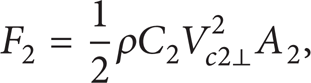
where C2 is the resistance coefficient of the second joint, V_c2⊥ is the velocity perpendicular to the plate, and A2 is the area of the plate which can be calculated when we got the velocity of each joint.

The resultant velocity of the center of gravity of the second joint is ${\vec{V}}_{c 2} = ({\dot{X}}_{0} - L_{1} \sin θ_{10} {\dot{θ}}_{10} - L_{c 2} \sin θ_{20} {\dot{θ}}_{20}, L_{1} \cos θ_{10} {\dot{θ}}_{10} + L_{c 2} \cos θ_{20} {\dot{θ}}_{20})$ , the normal vector of the second joint is ${\vec{I}}_{2} = (\sin θ_{20}, - \cos θ_{20})$ , and V_c2⊥ can be calculated by ${\vec{V}}_{c 2}$ and ${\vec{I}}_{2}$ we can get

V_{c 2 ⊥} = {\vec{V}}_{c 2} \cdot {\vec{I}}_{2} .

(11)

V_c2⊥ is a scalar, when V_c2⊥>0, and ${\vec{F}}_{2}$ is in the same direction of V_c2⊥; in this case, ${\vec{F}}_{2}$ is shown as follows:

{\vec{F}}_{2} = (\frac{1}{2} ρ C_{2} V_{c 2 ⊥}^{2} A_{2} \sin θ_{20}, - \frac{1}{2} ρ C_{2} V_{c 2 ⊥}^{2} A_{2} \cos θ_{20})

(12)

when V_c2⊥<0. ${\vec{F}}_{2}$ is in the opposite direction of V_c2⊥; in this case, ${\vec{F}}_{2}$ is shown as follows:

{\vec{F}}_{2} = (- \frac{1}{2} ρ C_{2} V_{c 2 ⊥}^{2} A_{2} \sin θ_{20}, \frac{1}{2} ρ C_{2} V_{c 2 ⊥}^{2} A_{2} \cos θ_{20}) .

(13)

We get the energy and forces by the above analysis; acceleration of the three variables can be calculated by the following equation:

\begin{matrix} (\begin{pmatrix} D_{11} & D_{12} & D_{13} \\ D_{21} & D_{22} & D_{23} \\ D_{31} & D_{32} & D_{33} \end{pmatrix}) (\begin{pmatrix} {\ddot{θ}}_{10} \\ {\ddot{θ}}_{21} \\ {\ddot{X}}_{0} \end{pmatrix}) + (\begin{pmatrix} D_{111} & D_{122} \\ D_{211} & D_{222} \\ D_{311} & D_{322} \end{pmatrix}) (\begin{matrix} {\dot{θ}}_{10}^{2} \\ {\dot{θ}}_{21}^{2} \end{matrix}) \\ + (\begin{pmatrix} D_{112} \\ D_{212} \\ D_{312} \end{pmatrix}) (\begin{pmatrix} {\dot{θ}}_{10} & {\dot{θ}}_{21} \end{pmatrix}) = (\begin{pmatrix} Q_{1} \\ Q_{2} \\ Q_{3} \end{pmatrix}) . \end{matrix}

(14)

2.3. Analysis of Negative Work

In one motion period, muscles of the fish and hydrodynamic forces generated by the fluid both do positive work and negative work as well. Altringham studied gadidae fish, he figured out that muscles of the body do positive work in most of the period; however, in the vicinity of the tail, proportion of negative work can reach as high as 50% under given conditions. Biologist John H. Long studied the relationship between thrust efficiency and negative work; he found that by adjusting the stiffness of the body in one period, muscles of the fish can use negative work better and hence improve thrust efficiency.

We used a model shown in Figure 2 to simulate the forces generated by fluid when fish swims using FLUENT software. The model has two joints; the body and motion parameters of the model are calculated by the principles mentioned above. Figure 3 shows four time-points of the pressure field and velocity field; the arrows in the figures show the direction and magnitude of velocity of the second joint. In the pressure field, red is high pressure and blue is low pressure; the result shows that pressure in the forward direction is higher than that of the backward direction; therefore, a resistance force is generated. The resistance force has a component in the direction of the fish swimming; hence, thrust force is generated. In the velocity field, behind the fish's tail, there are several green circles, that is, Karman vortex street. The red dash line connects the vortexes. Live fish acquire thrust force by the generated Karman vortex street and fish thrust the fluid generating vortexes; the rotation momentum of the vortex has reaction force to the tail of the fish; thus, fish acquire the thrust force to swim forward.

Figure 2:

FLUENT model of two-joint fish with mesh.

Figure 3:

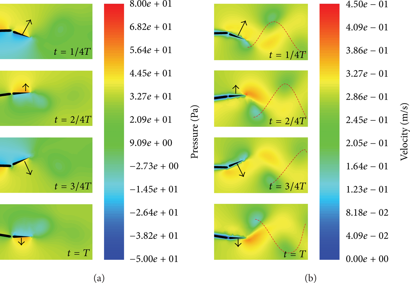
Simulation of the swimming under conditions f = 0.5 Hz and fluid velocity V_f = 0.27 m/s. (a) Pressure field; (b) velocity field.

By simulation, we got the forces generated to the tail of the fish, and we got the angular speed of the tail; hence, we can calculate the power of the fluid to the tail, which is shown in Figure 5. In one period, both positive and negative works are generated by the fluid to the tail. The area of the shaded parts in the figure shows the work made by the fluid, the area above the x-axis is the positive work, and that below the x-axis is the negative work. The total work in one period is positive, which can explain why fish swim forward.

Both positive work and negative work are generated by the two joints as well. In Figure 4 the torque and angular velocity of both the first and the second joint are given out; we can see from the figure that the torque and angular velocity have phase difference. Let the phase difference be ϕ; the power to drive the two joints is the product of the torque and angular velocity. Hence, the phase of negative work in one period is 2ϕ. In our model, the phases of negative work of the first and second joint are 194° and 44°. The phase difference of the first joint is much bigger than that of the second joint; one of the reasons is that the first joint drives both the first joint and the second joint and the second joint drives only the second joint; we also see from Figure 4 that the magnitude of the first torque is about 3 times higher than the second torque.

Figure 4:

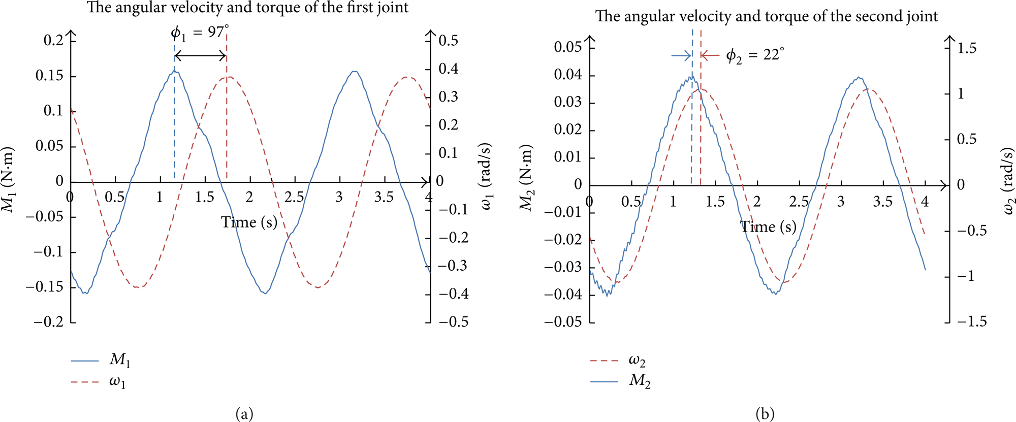
Torque and angular velocity of the two joints. (a) First joint; (b) second joint.

Figure 5:

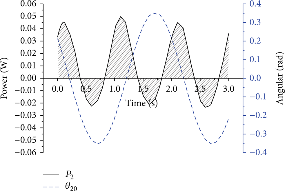
Power of the fluid to the second joint.

From the above analysis, we can get that both the muscles of the fish and hydrodynamics do positive work and negative work as well in one period; many researchers have figured out that fish improve thrust efficiency by utilizing negative work, which is much related to the stiffness of the fish; therefore, stiffness and control schemes should be discussed.

2.4. Stiffness and Control

Stiffness of the fish can be measured by Young's modulus, which is shown as follows [20]:

E = \frac{M R}{I} .

(15)

E is Young's modulus; M is torque to the point; R is the radius of the bent circle; I is section inertia. In a fish model, I is the decisive factor of Young's modulus. The section inertia of a dead fish is constant; however, in a live fish, the section inertia of a joint can be adjusted by muscles’ force. In our fish model, if the joint is not driven, the two sides of the joint will coincide; that is, R = 0, Young's modulus is zero.

A motor model is used for simulating the driving of the fish. The stiffness of robotic fish is basically decided by the materials the joint consists of; however, when the fish is driven by motors, the stiffness can be modified by adjusting the torque the motor generated. Using different control methods, we can get different torques; hence, we can adjust stiffness of the joint by adjusting control methods. It has been proved that the stiffness of a joint is proportional to the K_p factor of a PID position control method:

K_{p} \propto Stf .

(16)

In our research, the stiffness of each joint is constant as we used only one kind of material; however, the stiffness of the motors to drive the joints is not constant; we can adjust the stiffness of the motors conveniently by using proper control theory. In order to adjust the stiffness of the fish, we need to adjust the stiffness of the motors. This is an equivalent and convenient way to adjust the stiffness of the fish. As there is a linear relationship between the parameter of K_p and the stiffness of the system, therefore, we could use K_p to represent the stiffness of each joint.

Motion schemes of the two joints are shown in (3); there is position error of the real position and the schemed position and a specific torque value is calculated by PID position controller; the accelerations of the three variables are calculated by dynamic model shown in (7) and by double integral we can get the velocity of the three variables; then, the forces can be calculated by (9)–(13). By iteration, all the parameters we need are calculated.

2.5. Thrust Efficiency

Propulsion efficiency is the key problem we study in our research; it is defined as the proportion of the useful work to push the fish forward among the total work used to actuate the joints and other components of the robotic fish. In our research, the components that need to be actuated are two joints; the total work is the energy used on them. The total work in one period can be described as

W_{total} = \int_{0}^{T} ‍ (M_{1} (t) {\dot{θ}}_{10} (t) + M_{2} (t) {\dot{θ}}_{21} (t)) d t,

(17)

where M₁(t) is the torque of the first joint and M₂(t) is the torque of the second joint.

The useful work in one period can be described as

W_{useful} = \int_{0}^{T} ‍ (F_{p} (t) \cdot U (t)) d t,

(18)

where U(t) is the velocity of the fish and F_p is the component of the hydrodynamic force to push the fish forward; as we neglected the hydrodynamic force caused by the first joint, we can get F_p = F_2x, which is the x-axis component of the hydrodynamic force caused by the second joint.

The propulsion efficiency η is shown as follows:

η = \frac{W_{useful}}{W_{total}} = \frac{\int_{0}^{T} ‍ (F_{2 x} (t) \cdot U (t)) d t}{\int_{0}^{T} ‍ (M_{1} (t) {\dot{θ}}_{10} (t) + M_{2} (t) {\dot{θ}}_{21} (t)) d t} .

(19)

The thrust efficiency can reach 80–90% in live fish while that of the existing robotic fish is 40–50% [6, 8]; there is much room for improvement of robotic fish. Thrust efficiency is determined by many factors such as the parameters of the body curve, the number of the joints, the frequency and the amplitude of undulatory, and the stiffness of the fish's body. Many scholars have studied thrust efficiency of robotic fish; most of them focused on body parameters and undulatory parameters, but few paid attention to the effect of the stiffness of the fish's body to the thrust efficiency. Long Jr. et al. figured out that in the negative work period fish can adjust the body's stiffness to improve the velocity and other factors which can determine the thrust efficiency [21].

The direct way to change the stiffness of the robotic fish is to make fish using different materials with exactly the same body parameters and motion parameters; however, this is a huge task and making the parameters exactly the same is unrealistic, and further the stiffness is not a constant in one period, so we need to find out a way that the stiffness can be adjusted conveniently and the other parameters can be kept exactly the same.

2.6. Different Control Methods

When the K_p of the first joint is constant in one period, we did some trials by increasing and decreasing the K_p of the first joint. When the K_p of the first joint is variable in one period, we used different methods to control the laws that K_p should obey. We did some trials using the following method:

K_p of the first joint is normal;

increasing K_p of the first joint;

K_p of the first joint varies in inverse proportion to hydrodynamic force;

K_p of the first joint varies in proportion to hydrodynamic force;

K_p of the first joint varies in proportion to a given sine curve.

3. Discussion

3.1. Constant Stiffness

The propulsion efficiency should be calculated in stable period; Figure 6 shows the thrust efficiency of constant K_p in one period using Matlab; we can deduce from the results that when K_p is given a normal value, the thrust efficiency is low, by increasing the K_p of the first joint, thrust efficiency gets its peak value, and when K_p is given the value of 70 and when K_p is given bigger values, the thrust efficiency gets a slight descent.

Figure 6:

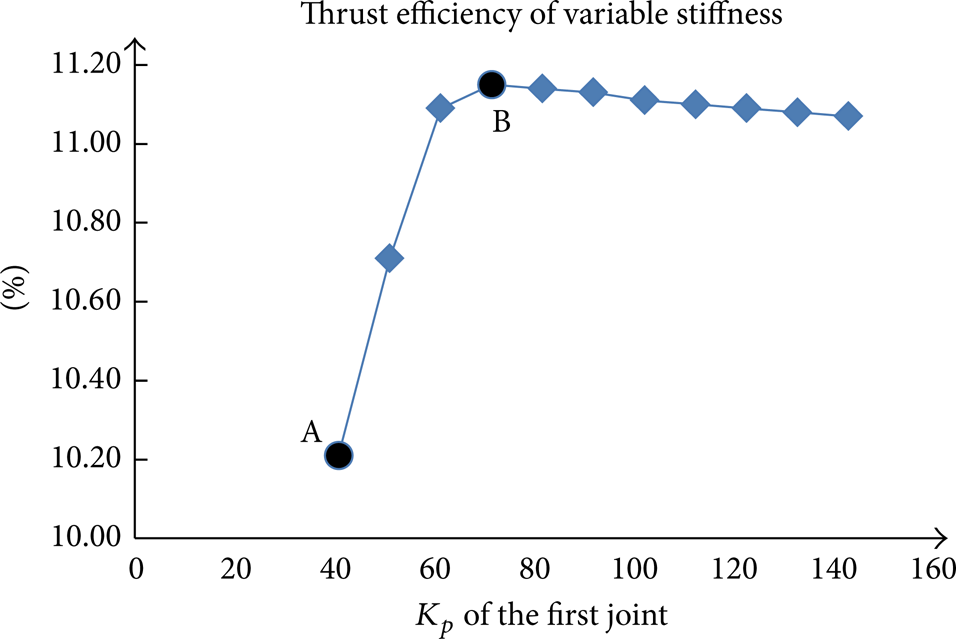
Thrust efficiency of constant stiffness. Point A is the thrust efficiency when K_p is a normal value and point B is the highest thrust efficiency when K_p is increased.

3.2. Adjusting Stiffness

We used the methods shown in Section 2.6 to improve thrust efficiency of the robotic fish, and the simulation results of the thrust efficiency using the methods above are shown in Figure 7. The number on the x-axis represents the methods and the height of the columns represents the thrust efficiencies.

Figure 7:

Thrust efficiency of different methods; the numbers on the x-axis represent the methods shown in Section 2.6.

As shown in Figure 7, the original thrust efficiency of the robotic fish is 10.2%; by increasing K_p of the first joint, thrust efficiency gets 11.2% which is 1% higher than the original thrust efficiency. Methods (3), (4), and (5) use variable stiffness in one period; thrust efficiency of methods (4) and (5) is higher than original efficiency but lower than efficiency of method (2); robotic fish gets the highest propulsion efficiency using method (3).

The result shows that thrust efficiency gets higher by increasing stiffness of the first joint, and by adjusting stiffness properly in one period thrust efficiency gets its highest level.

4. Conclusions

In this paper, a simplified model of robotic fish is implemented; kinematic model and dynamic model of the robotic fish are analyzed and we discussed the method of evaluating the propulsion efficiency. Preliminary simulating experiments were conducted to investigate the high efficient propulsion method with stiffness control. By comparing the propulsion efficiencies of robotic fish using different stiffness control methods, we found that when the hydrodynamic force does positive work, the stiffness of the fish robot should be reduced to couple with the hydrodynamic force. While the hydrodynamic force does negative work, the stiffness of the fish should be increased to a moderate value, thus, to obtain better swimming efficiency.

Conflict of Interests

The authors declare that there is no conflict of interests regarding the publication of this paper.

Footnotes

Acknowledgments

This work is supported by the National Nature Science Foundation of China (under Grant nos. 61203353 and 61333016) and China Scholarship Council (under Grant no. 201206025009).

References

Shadwick

R. E.

and Lauder

G. V.

, Eds., Fish Physiology: Fish Biomechanics: Fish Biomechanics, Academic Press, San Diego, Calif, USA, 2006.

Tytell

E. D.

and Lauder

G. V.

, “The hydrodynamics of eel swimming: I. Wake structure,” Journal of Experimental Biology, vol. 207, no. 11, pp. 1825–1841, 2004.

Triantafyllou

M. S.

Triantafyllou

G. S.

, and Yue

D. K. P.

, “Hydrodynamics of fishlike swimming,” Annual Review of Fluid Mechanics, vol. 32, no. 1, pp. 33–53, 2000.

Anderson

J. M.

Streitlien

Barrett

D. S.

, and Triantafyllou

M. S.

, “Oscillating foils of high propulsive efficiency,” Journal of Fluid Mechanics, vol. 360, no. 1, pp. 41–72, 1998.

Wen

and Lauder

, “Understanding undulatory locomotion in shes using an inertia-compensated apping foil robotic device,” Bioinspiration & Biomimetics, vol. 8, no. 4, Article ID 046013, 2013.

Wen

Liang

, and Li

, “Hydrodynamic experimental investigation on efficient swimming of robotic fish using self-propelled method,” International Journal of Offshore and Polar Engineering, vol. 20, no. 3, pp. 167–174, 2010.

Wen

Wang

T. M.

G. H.

, and Liang

, “Hybrid undulatory kinematics of a robotic Mackerel (Scomber scombrus): theoretical modeling and experimental investigation,” Science China Technological Sciences, vol. 55, no. 10, pp. 2941–2952, 2012.

Wen

Wang

, and Liang

J. H.

, “Quantitative thrust efficiency of a self-propulsive robotic fish: experimental method and hydrodynamic investigation,” IEEE/ASME Transactions on Mechatronics, vol. 18, no. 3, pp. 1027–1038, 2013.

Wen

Liang

Shen

Bao

, and Zhang

, “Hydrodynamic performance of an undulatory robot: functional roles of the body and caudal fin locomotion,” International Journal of Advanced Robotic Systems, vol. 10, 2013.

10.

Wen

Wang

T. M.

G. H.

, and Liang

J. H.

, “Hydrodynamic investigation of a self-propelled robotic fish based on a force-feedback control method,” Bioinspiration & Biomimetics, vol. 7, no. 3, Article ID 036012, 2012.

11.

Wen

Wang

Liang

, and Wang

, “Novel method for the modeling and control investigation of efficient swimming for robotic fish,” IEEE Transactions on Industrial Electronics, vol. 59, no. 8, pp. 3176–3188, 2012.

12.

Liang

Wang

, and Wen

, “Development of a two-joint robotic fish for real-world exploration,” Journal of Field Robotics, vol. 28, no. 1, pp. 70–79, 2011.

13.

Wang

Wen

Liang

, and Wu

, “Fuzzy vorticity control of a biomimetic robotic fish using a flapping lunate tail,” Journal of Bionic Engineering, vol. 7, no. 1, pp. 56–65, 2010.

14.

Wardle

C. S.

, “Limit offish swimming speed,” Nature, vol. 255, no. 5511, pp. 725–727, 1975.

15.

Coleman

and Wilson

D. S.

, “Shyness and boldness in pump-kinseed sunfish: individual differences are context-specific,” Animal Behaviour, vol. 56, no. 4, pp. 927–936, 1998.

16.

Ziegler

Homann

Carbajal

J. P.

, and Pfeifer

, “Varying body stiffness for aquatic locomotion,” in Proceedings of the IEEE International Conference on Robotics and Automation (ICRA '11), pp. 2705–2712, 2011.

17.

Triantafyllou

M. S.

and Triantafyllou

G. S.

, “An efficient swimming machine,” Scientific American, vol. 272, no. 3, pp. 40–48, 1995.

18.

Liu

and Hu

, “Biological inspiration: from carangiform fish to multi-joint robotic fish,” Journal of Bionic Engineering, vol. 7, no. 1, pp. 35–48, 2010.

19.

Liu

Y.-X.

Chen

W.-S.

, and Liu

J.-K.

, “Research on the swing of the body of two-joint robot fish,” Journal of Bionic Engineering, vol. 5, no. 2, pp. 159–165, 2008.

20.

McHenry

and Pell

, “Mechanical control of swimming speed: stiffness and axial waveform in undulating fish models,” Journal of Experimental Biology, vol. 198, no. 11, pp. 2293–2305, 1995.

21.

Long

J. H.

Jr. Adcock

, and Root

R. G.

, “Force transmission via axial tendons in undulating fish: a dynamic analysis,” Comparative Biochemistry and Physiology A: Molecular and Integrative Physiology, vol. 133, no. 4, pp. 911–929, 2002.

A Stiffness-Adjusting Method to Improve Thrust Efficiency of a Two-Joint Robotic Fish

Abstract

1. Introduction

2. Materials and Methods

2.1. Model and Parameters of Robotic Fish

2.2. Dynamical Model

2.3. Analysis of Negative Work

2.4. Stiffness and Control

2.5. Thrust Efficiency

2.6. Different Control Methods

3. Discussion

3.1. Constant Stiffness

3.2. Adjusting Stiffness

4. Conclusions

Conflict of Interests

Footnotes

Acknowledgments

References