
Abstract
In this paper, we introduce a mobility aware and energy efficient congestion control protocol “time sharing energy efficient congestion control (TSEEC) for mobile wireless sensor network.” TSEEC is based on hybrid scheme of time division multiple access protocol (TDMA) and statistical time division multiple access (STDMA) protocol that inform the sensor nodes when to wake up and to go to listening state so as to save energy. This management helps in minimizing congestion and improving network energy conservation through its load based allocation (LBA) and time allocation leister (TAL) techniques. LBA is typically based on STDMA that uses sensor node information for assignment of dynamic timeslots to the sensor, nodes, whereas TAL targets the mobility management of sensor nodes that further comprises three main strategies of cluster member node that is, joining cluster, leaving cluster, and absence of data/redundant data with extricated time allocation (ETA), shift back time allocation (SBTA), and eScaped Time Allocation (STA) subtechniques. In addition, TSEEC protocol introduces the mobility pattern to control the mobile sensor node (MSN) movement to enable the protocol to effectively adapt itself to change the traffic environments and mobility. Mathematical analysis and NS2 simulation show that TSEEC outperforms SMAC in terms of energy consumption and packet deliver ratio. Furthermore, a comparative analysis of TSEEC with various well-known related MAC protocols is also given.
1. Introduction
Wireless sensor network consists of autonomous sensors and uses a shared medium for monitoring physical environment like temperature, sound, pressure, or vibration and shares this data with a base station. These are surveillance devices that are of three basic elements: sensing subsystem, processing subsystem, and storage.
The advancement in static WSN along with distributed robotics [1] has led to a new set of Mobile WSN (MWSN). MWSNs have same network architecture as WSNs have; however they are provided with explicit or implicit mechanisms that provides mobility to these sensor nodes to move in space (e.g., terrestrial robotic car, underwater, or air current) over time [2]. In addition, MWSNs are able to derive their coordinates through relative means (localization techniques [3]) or absolute means (e.g., geographic positioning system (GPS)). There are quite a few classes of MWSN that can be plainly categorized into the following classes: (i) highly mobile; in this scenario, devices can move at a velocity such as human, cars, and airplanes, (ii) mostly static; in this scenario, the devices can move at a very low velocity such as moving robots, and (iii) hybrid, in this scenario, we have both classes, that is, highly mobile and mostly static, such as moving cars having sensors installed in it [2].
MWSN application has perceptibly diverse characteristics as well as requirements from traditional wireless network applications that pose some exceptional challenges, that is, energy efficiency and congestion. An MSN in MWSN environment is equipped with battery and recharging or changing the battery frequently is very difficult, and in some scenarios, it is almost not possible. Therefore, energy conservation is measured as the vital design confront in MWSN, which is essential for prolonging network lifetime than such other performance parameters such as latency, throughput, and bandwidth. Consequently, majority of the ongoing research on MWSN aims to minimize the energy consumption ratio. Apparently, radio functions such as sending, receiving, or idle listening to the channel drain the energy a lot. On the other hand, congestion is another key factor that affects the energy conservation. Congestion usually arises when there is simultaneous transmission of data from multiple nodes to the sink node resulting in packet loss. The lost packets require retransmission of the same data packet that minimizes the overall energy efficiency of the network. In order to minimize the energy consumption ratio, an efficient MAC protocol that allocates medium resources shared by different sensor node in MWSN is required.
Due to aforementioned constraints, this research study is to implement a novel mobility aware energy efficient MAC protocol for MWSN. The scheduling (awake/listening states) algorithm developed for the proposed MAC is aiming to achieve relative better energy efficient for time-critical application traffics. Next is to accomplish the minimization of lower energy consumption. TSEEC uses mobility pattern that enables protocol to robustly adjust the mobility pattern, making it suitable for sensor environments suitable for both high and low mobilities. TSEEC assumes that MSNs know their location information by using any localization technique [2]. This location information is used to predict the mobility pattern by using [4].
In the proposed scheme, we have classified cause of congestion into two classes, that is, (i) node level congestion (NLC) and (ii) link level congestion (LLC). The NLC is caused by the buffer overflow whereas LLC is caused by large data being pumped into the channel by various neighboring nodes at the same time. Therefore, in this paper, a protocol is designed based on STDMA that improves performance in both NLC and LLC and ultimately results in energy efficiency of the network. With the help of STDMA, each MSN shares its statistical information in Hello Packet with cluster head (CH). This Hello Packet contains unique ID, battery information, and location information in the cluster. The CH then uses MSN feedback and uses a modified TDMA technique of timeslots allocation to its MSNs in specific cluster. This innovative statistical technique in TDMA provides energy efficiency to network and also minimizes congestion at sink node in MWSN. The technique works in a scenario wherein the mobile node may or may not sense any environmental physical quantity and leaves or joins new cluster and so on, while CH remains as the coordinator throughout this span of communication. Deficiencies in the static WSN [5, 6] are also handled by mobile sensor nodes.
The rest of the paper is organized as follows. Section 2 briefly describes review of some related work. Section 3 presents the proposed protocol (i.e., TSEEC). Section 4 shows the energy model for TSEEC. Finally, we present simulation results and discussions in Section 5, followed by conclusion in Section 6.
2. Related Work
Existing protocols that controls energy conservation, end-to-end network delay, and congestion in MWSNs are few among many of the issues. Congestion at the cluster head can lead to more overheads that consume a considerable amount of energy as well as packet loss and delay in the network.
In [5], randomized coordination algorithm that improves sensor networks efficiency and energy is described. This algorithm makes decision to sleep and wake up. The sensor node that wakes up is responsible to serve as a coordinator. The preference is given to hop-to-hop communication (short range) over direct communication (long range), which saves the network capacity. The number of coordinators should, however, be kept as minimum as possible to achieve maximum network life time. In [7] GAF scheme is proposed that uses geographical location information related to division of area into fixed square grids with constant size has been provided. All sensor nodes should follow the scheme of sleep and awake state to minimize the battery usage, but one sensor node should always be in awake state in order to route the data.
An algorithm PCAP is a MAC protocol based on CSMA which uses existing handshake mechanism of RTS and CTS which helps in avoiding collision in the network [8]. While waiting for CTS, PCAP permits the nodes to perform other tasks. The maximum throughput of PCAP is about 20%. CSMA technique however increases delay in the network since it uses RTS and CTS packets. To avoid congestion, various techniques and algorithms are used in WSN like CSMA/CA in IEEE 802.15.4 for CD-WPAN. This technique is used to introduce the beacon enable mode [9]. Sharing of information is done through cross-layer communication. This technique may however prove not so useful to avoid congestion in the network and loss of source packet. Key reason of dropping of packets is many-to-one communication under heavy traffic load.
One major concern of congestion on sink node is due to transmission of packets to common receiving node. This congestion is controlled by robust routing algorithm with fair congestion control (RRA-FCC) [10]. Typical wireless sensor network has 1 or 2 sink nodes, but there are numerous research scenarios where tens to hundreds of sink nodes are deployed in WSN region.
A scheme is proposed using mobile sink or minisink in WSN to avoid congestion [11]. Minisink is responsible for retrieving data from the sensor nodes. After retrieving data from nodes, aggregation function is applied to reduce the number of node's packets carried out on the network. Reduction in number of packets transmitted and limiting the number of hops in conservation of energy during transmission. WSN runs on batteries and if deployed in a region where reviving these batteries is impossible, then there is a great chance of failing of WSN. For such problems, TRAMA is suited protocol which can be used for energy conservation and for avoiding congestion [12]. It is a TDMA technique that divides the timeslots into two parts. One is random access protocol and the other is scheduled access period. The main drawback of this technique is cutting off the long communication process which results in dropping of packets.
A scheme is proposed based on zone based routing based on modification of adhoc on demand distance vector routing protocol (AODV) [13]. This scheme is capable of reducing network segment error as well as reducing the amount of control information. This can be obtained by the effect of path finding and also addresses various problems of reliability, improved error control mechanism, and link repair with minimum overhead in mobile sensor networks. In this protocol, the member node transmits data to zone head in three phases, that is, mobility factor and zone head selection, route maintenance and node mobility.
A location based scheme is proposed based on routing protocol in which the concept of greedy forwarding on the basis of cost function for each node has been used [14]. This cost is close to the Euclidean length of the shortest path from sensor node to the base station. After a few hops when the greedy routing is not possible, the packet uses the high-cost-to-low-cost rule and forwards it to coordinator/sink node.
The original AODV protocol suffers from performance degradation in mobile environment, but it performs well in static environment [15]. Moreover, there is no mechanism in AODV protocol to derive the cost and willingness of a node to be a part of data transmission.
DMAC considers congestion on the sink node that consumes extra energy [16]. Robust routing algorithm with fair congestion control (RRA-FCC) [17] is proposed along with time-driven or event-driven models. RRA-FCC is not only to minimize the congestion and maximize energy efficiency in the network.
In WSN environment, the energy conservation depends on the distance between sensor nodes, The greater the distance between two nodes, the greater the energy consumption and vice-versa. In addition, another vital cause of sensor node's energy wastage is the state of the sensor node, that is, idle listening, collision, over hearing, central packet overhead, and overmitting [17]. To cope with the said problem, there are other schemes that generally minimize the energy consumption of a sensor node, that is, duty cycling and data-driven technique. But these schemes still needed better time allocation technique that helps in minimizing congestion in the WSN [17], CCP [18], SPAN [19], HEED [20], ECODA [21], and LCM [22] well-known protocols that are used to minimize congestion. However, the said schemes do not cope with the delay arise in the network. Therefore, based on these reservations, the proposed hybrid protocol “TSEEC” has been used to effectively circumvent all these constraints. (MICA2 Mote) is a basic example whose energy consumption is given in Table 1 [23]. Different techniques to compress data for energy conservation are discussed [24–27]. Due to compression, WSNs omit important data, which can be a loss for data manipulation.
MICA sensor specification.

In order to collect data information in an efficient manner, several algorithms that are used for efficient collection of data from WSN environment are proposed. These schemes use clustering approach that is based on residual energy. The cluster head rotating mechanism is also in introduced that enhance network life time. However, most of the algorithms have not yet considered the expected residual energy that is predicted the residual energy for being selected the cluster head. To avoid such problems, a fuzzy-logic based clustering approach along with extension of energy prediction is proposed. This scheme is used for prolonging network life by means of evenly distribution of workload amongst various sensor nodes [28].
However, given brittle conditions of a mobile WSN, where link breakage is quite high among various mobile sensor nodes due to their abrupt movement, TSEEC technique works well by introducing mobility factor along with the scheduling technique. Furthermore, it also helps in minimizing the time required for mobile sensor node long communication period with CH which results in dropping of packets.
3. Proposed Solution
Application Scenario. Due to broadcast nature of WSN, it is a difficult job to incorporate congestion control at sink node. Therefore, a new MAC protocol is required to design focusing on energy efficiency and congestion control. The designed protocol results in prolonging network lifetime and enhancing network efficiency. In mobile network, there are two phases of a node: (i) mobility phase: node moves from one location to another location in the network and (ii) stagnant phase: between two mobility phases, there is stagnant phase where node stays at same location for some time interval. In the scenarios, where stagnant phase does not exist or at least exists for very short time, there the time sharing based algorithm is not possible to implement. In our underlying scenario for the designing of TSEEC, stagnant phase is long enough for a node to stay in some cluster that time sharing based algorithm can be used without any objection. Moreover, node location information is used for decision making of mobility model in our algorithm as shown in Figure 1. Hence, time sharing based algorithm can be implemented over the underlying scenario.

Typical working of TSEEC.
3.1. Overview
Consider an MWSN composed of n number of MSNs, that are deployed in x and y coordinate plane. The deployed nodes grouped together to form their respective cluster. In each cluster, they have their static cluster head (CH) as shown in Figure 2.

Deployment of sensor nodes along with cluster head.
Formation of cluster is described in Section 3.1.1. CH assigns timeslots to its joined MSNs with the help of STDMA. The STDMA acquires MSN's statistical information, that is, unique ID, battery information, and location information. After getting statistical information from each MSN, the CH evaluates this statistical information and assigns dynamic timeslots to each MSN.
TSEEC comprises two main strategies which deal with delay in a network. This delay is caused by freeing up of assigned timeslots and other issues which have been mentioned above. These strategies are load based allocation (LBA) and time allocation leister (TAL). Figure 3 summarizes the process of TSEEC.

Working of TSEEC.
3.1.1. Cluster Head Formation
Cluster Head (CH) is based on self-capability of organizing sensor nodes. Assume that all the MSNs know there location as well as their neighbors in its vicinity head (VH). We use the term vicinity for neighboring area of a sensor node, that is, signal range of a sensor node. However, the terminology vicinity head (VH) can be relevant to CH. The deployment of sensor nodes is settled on; thus, at the beginning, selection of CH is on hand. Since the nature of MSN is homogenous, therefore, the MSN with maximum neighboring nodes is selected as CH. After the selection of CH, each MSN attaches to the CH on the basis of received signal strength (RSSI). In case an MSN receives request from neighboring CH (CHs which are nearer to this node), then the following algorithm is followed:
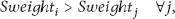
If


If

3.1.2. Load Based Allocation
In this phase, CH assigns timeslots to each mobile cluster member node. The process of assigning timeslots works as follows: each MSN send a Type-I Hello Packet to the CH. The format of the Hello Packet consists of different information, that is, Type-I_Broadcast_msg{node ID, battery information, location information, propagation time}.
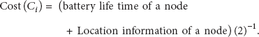
The CH computes the distance between MSN and itself using time of arrival (TOA). After calculating distance, the CH assigns weight to each MSN on the basis of distance and the information available in Type-1_Broadcast_msg. Similarly, TSEEC uses the weighted value and broadcast_msg as a metric for assigning timeslots to each MSN in the network. The weighted value is calculated by using (5)

The algorithm for assignment of timeslots is shown in Algorithm 1.
Mobile_sensor_node MSN node_ID, Battery_life, Location_Info, time_of_sending Hello_Packet(){ node_ID = MSN Battery_life = MSN Location_info = MSN Location_info = MSN while(!total_mobile_sensor_nodes) MSN Hello_ Packet() to CH TOA(){ distance_MSN = mobile_sensor_node e-MSN CH assign Weights to MSN End while
Algorithm 1
After calculating the weighted value for each MSN, this information is broadcasted in the cluster in Type-II_broadcast_msg. The format of the Type_II broadcast message is as follows: Type-I_Broadcast_msg{node id's, starting time of cycle, scheduling information, dynamic timeslots}. Upon receiving Type_II broadcast message, each node becomes aware of each MSN's information that is in same cluster.
To elaborate the assignment of dynamic timeslots based on their statistical information, an example scenario is illustrated in Figure 4. In this scenario, we have considered a single cluster having five MSNs (n 1, n 2, n 3, n 4, and n 5) and one cluster head (CH1). Assume that all MSNs broadcast Type-I message for the CH1. Upon receiving Type-I message by CH1, CH1 calculates weight by using two types of information, that is, (i) the information of all nodes based on information inside the header of the broadcast message and (ii) the distance calculated by using ToA mechanism. The following metric Table 2 is assumed after calculating Type-I broadcast message information.
Example scenario of calculated weighted value.

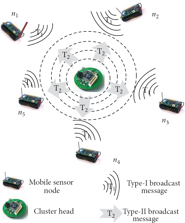
Scenario illustrating the Type-I and Type-II broadcast messages to calculate weight for each MSN and assign dynamic timeslots to all mobile sensor nodes.
The information available in Table 2 is broadcasted by CH1 in the cluster in Type-II broadcast message. Upon receiving Type-II broadcast message by all five MSNs, all the MSNs get the information of starting time of the data communication cycle and scheduling information along with other node's information. This mechanism helps in providing efficiency in time synchronization among all the MSNs that is, the (n
4) which is in communication with the CH1, and the rest of MSNs (
After completing one cycle, the same mechanism continues for next cycle.
The strategy LBA, which is based on STDMA, helps in acquiring statistical information from different MSNs and assigns timeslots after the evaluation of statistical information. However, mobility aware TAL technique deals with the exploitation of free timeslots that is done after node's joining or leaving the cluster or absence of data in that particular sensing region. TAL mainly comprises three basic loops of joining, leaving and absence of data in the scenarios: extricated time allocation (ETA), shift back time allocation (SBTA), and eScaped time allocation (STA) as shown in Figure 5.

Sharing of timeslots among different mobile nodes.
3.1.3. Time Allocation Leister
The rapid change in the location of sensor node results in modification in the network topology. The abrupt change in topology as well as location of different sensor nodes influences the MWSN's scheduling process and affects the allocation of timeslots in the network. The problem of rapid change in topology as well as location (joining and leaving of the sensor node from cluster to another cluster) is handled by TAL mobility model. The three prongs of TAL are extricated time allocation (ETA), shift back time allocation (SBTA) and escaped time allocation (STA).
ETA. In this scenario, when there is absence of data, the allotted timeslots should be unutilized by that sensor node. In this technique, the MSN senses the same data which we call it “redundant data” or, sometimes, it does not sense data at all. After that, MSN broadcasts the free timeslot message for its neighboring MSN to shift back there timeslots as per free time timeslots kept over. Moreover, when new MSN enters in the cluster, the CH assigns that free timeslots to the new entrant MSN. This free timeslot must mull over two scenarios for its further utilization in order to provide efficiency to the mobile WSN as shown in Figure 5.
In first scenario, CH assigns free timeslot to those MSNs that recently enter into new cluster. Secondly, assignment of free timeslots to the neighboring in that cluster by CH takes place (neighboring node will shift back its timeslot). SBTA. This is the case in which MSN leaves its current cluster. Initially, it broadcasts its timeslots as well as leaving status. The neighboring nodes in the cycle shift back its timeslot as per free timeslots which are kept over by the departed MSN. STA. STA comprises both ETA as well as SBTA. In this technique, MSN has no data to sense or has redundant data and other MSN for leaving the cluster.
Mobility Model for TAL. TSEEC uses location information to predict the performance of a mobile sensor node. However, localization technique is well studied in WSN [4]. However, most of the work assumes that the physical location of a sensor node is known. Therefore, TSEEC assumes that every MSN in the network knows their location information by using [29].
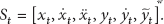
Let
In the proposed scheme, we used AR-1 model [4] that is used for MSN mobility pattern prediction. The state of the MSN at time t is defined by a column vector
Hence, AR-1 model [4] provides

In this equation, A represents a 6
Hence, at any given time t, the mobility state information of MSN 
After estimating mobility of MSN, it is now required to broadcast the mobility information in the cluster. For this procedure, modification in the MAC header that contains the information about mobility of MSN has been done. Let
After calculating the value of
Algorithm 2 represents the working of TSEEC.
N = node Number of nodes = 50 Z = Zone (z1, z2) Cluster Head = CH1, CH2 Loop i← 0 to 24 z1 = node[i] Z1 = z1 + CH1 Loop i = ← 25 to 50 z2 = node Z2 = z2 + CH2 Loop j = 0 to 24 Node Loop j = 25 to 50 Node[j] ← Proc TAL Loop i← 0 to 24 If (payload_node = = 0) // condition 1 CH1← message ← node[i] then New_arr_node[i] ← else // condition 2 CH1← leave_msg ← node[i] Node[ CH1 → shiftback T of other nodes by a factor of else combine (condition 1 + condition 2) Repeat procTAL for zone 2
Algorithm 2
4. Hop-by-Hop Performance Evaluation in Mobile WSN
We have used the probabilistic approach for evaluating energy efficiency between two MSNs. We have classified our evaluation into three broad categories, that is, Probability of packet reception

In (10), R is the number of packets which are received by a node and N is the number of data packets which are propagated.
For the measurement of average delay between two nodes deployed in wireless sensor network, the following equation is used:
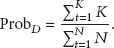
In (11), t is the time required to deliver K amount of packets successfully, N is the total number of packets which are transmitted and to be delivered in time t.
Retransmission consumes much energy. When packet is lost or delivered erroneously, that packet must be retransmitted. The node sends negative acknowledgment (NACK) to sender in its existing timeslots. While receiving NACK, the sender will retransmit that packet again. The probability of retransmission (by sender) can be found through the below equation:
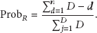
In (12), d is the sum of all packets, which are received by destination node, D is number of delivered packets, and d is the number of lost packets.
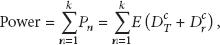
We next investigate how TSEEC reduces energy consumption. TSEEC plays a dominant role in consuming less energy due to time sharing TDMA based on STDMA. Let 
5. Energy Model
In TSEEC, an assumption has been made, that is, each MSN sends and receives data packets with an equal battery power, that is, sending and receiving. Therefore, the energy used by an MSN is autonomously depending on distance between adjacent MSNs. Consequently, we assume the below energy model to calculate power consumption for MSN in MWSN

Let 
In this paper, we assume that all MSNs forward data in multihop to a CH. Equation (16) describes the relationship between the total amount of data received by all nodes and the sum of hops

Based on (16), the total energy consumption can be expressed in terms of the total sum of all hops from all member nodes to their CH as follows:
6. Experimental Results and Discussions
To study the evaluation performance and comparison of TSEEC protocol with other protocols and scheduling techniques, we have used NS2 simulator.
6.1. Simulation Environment
Mobile wireless sensor nodes were randomly deployed within an area of 1000 m
The distances between MSNs are not kept constant variable and hence totally depend on the mobility pattern of each MSN in the given cluster. In the scenario of 50 MSNs, we have two clusters, each having a static CH. However, in the 100 MSNs scenario, there are 3 static clusters instead with the same ratio of one static CH in each cluster. The initial energy of each MSN was set to 15 Joules. In addition, we have used MAC type 802.11n in order to minimize network delay. 802.11n is used only by CH that avails frame aggregation technique [33] to deliver data packets at surface station. Each MSN generates data packets using constant bit rate (CBR), while hello packet is used only once at the start of the communication.
6.1.1. Message Interval Time (MIT)
Figures 6(a) and 6(b) show the MIT of TSEEC with and without using periodic active/listening scheduling technique. In Figure 6(a), we have 50 MSNs with two clusters. Each cluster has 1 CH, that is, CH1 and CH2; both CH1 and CH2 have 25 members each. The scheduling technique with periodic active/listening scheduling technique consumes less energy as compared to the one without it. When periodic active/listening scheduling is being used, MSNs, waiting for their turn to start communication with the respective CH, switch their radios on to a listening mode. This technique helps consume least energy, that is, 35 Joules, only for listening without the need to transmit any data packets. However, without active/listening scheduling technique, all MSNs turn their radios to full active mode and sense the environment. For instance, when there are 50 sensor nodes, TSEEC without periodic active/listening technique consumes 68 Joule of energy. To reduce this energy consumption, TSEEC with periodic active/listening scheduling technique is preferred as it inactivates the extra sensing of an MSN. Hence, the active/listening scheduling technique consumes 35 Joule of energy throughout the communication period. On the other hand with an increase in the number of MSNs to 100, as shown in Figure 6(b), the amount of energy consumed by MSN also increases in without periodic active/listening, that is, 118 Joule of energy consumption. This is the result of additional packet losses due to poor allotment of timeslots to all MSNs. However, TSEEC gives us satisfactory results while used with periodic active/listening scheduling technique if the number of MSNs increases, that is, 43 Joules of energy consumption.

Interarrival time in seconds under low traffic load.
6.2. Energy Level of Mobile Sensor Nodes
Figure 7 shows the energy consumption of both of the protocols, that is, TSEEC and SMAC. For comparison purpose, we implement SMAC in MWSN and compare its results with TSEEC. In SMAC, there is a long but same schedule during sleep/listen period that drops extra amount of data packets during sleep state. The protocol like SMAC is not suitable for MWSN, as the latter has abrupt movement of sensor nodes that affects the scheduling process. In mobility aware WSNs, the data frame advertising a mobile node's location information could be dropped by a node which is in sleep state. As a result, the node in sleep state would not have the information about the mobility pattern of all nodes in a given cluster. In terms of the overall effect on energy consumption of the MWSN, whenever there is a fixed sleep/listen schedule, a network having mobile nodes is affected considerably. As shown in Figure 7(a), the SMAC consumes maximum energy of 9 Joules per single cycle (if we have 50 nodes in a network, that is, 25 nodes in each cluster). On the other hand, TSEEC consumes considerably lower energy as it uses a periodic with active/listening scheduling technique. For instance, if we increase the number of MSNs as shown in Figure 7(b), the performance of SMAC is considered worse (consumes 14.5 Joules of energy) as compared to TSEEC (consumes 11.5 Joules of energy).

Calculating energy level at every mobile sensor node.
6.3. Delivery Ratio
Figures 8(a) and 8(b) show the packet delivery ratio of both protocols. In SMAC, the long listen/sleep period results in energy saving. But, in this case, traffic load and the mobility pattern of MSNs result in dropped data packets. Since MSNs are unable to receive data packets (mobility information and timeslot allotment of other nodes), that leads to deficient information about the cluster environment.

Calculated packet delivery ratio under low traffic Load (LTR).
This mechanism affects the overall data transmissions; hence, maximum amount of data packets is dropped due to lack of cluster information. As shown in Figure 7(a), increase in the speed of MSNs affects the scheduling process of SMAC; hence, delivery ratio decreases to 0.5%. However, TSEEC has 0.69% delivery ratio. For instance, if we increase the number of MSNs to 100 nodes as shown in Figure 7(b), the delivery ratio drastically decreases to 0.4%. However, TSEEC is not affected by increase in number of nodes in the cluster and has delivery ratio of 0.3%.
6.4. 802.11n Energy Level
Figure 9 shows the implementation of 802.11n at back end, that is, at the cluster head. There are various tests by employing scheduling techniques on CH, that is, idle listening, transmitting state, listening state and receiving state. It is noticed that CH in receiving state consumes less energy, that is, 2 Joules per one complete cycle of communication. In transmitting state, CH consumes 4.2 Joules of energy, since it uses the 802.11n aggregation technique (see [33] for more details) to deliver data to surface station. In listening state, the CH consumes negligible energy, as CH is always in listening and transmitting state. At the start of a communication period, it listens for member MSNs to get statistical information and assign timeslots. Since the CH cannot be kept in an idle state, it uses its radio throughout the communication period consuming 0.2 Joules of energy. The total consumed energy can be calculated as


Energy status of IEEE 802.11n.
7. Comparative Analysis with Existing MAC Protocols
In Table 3, we compared our protocol with the existing protocol in terms of synchronization, communication pattern, protocol type, and adaptively changes to atmosphere. In the given table, two S-MAC protocols, namely, T-MAC and DSMAC have same features with S-MAC. Cross-layer MAC protocols are not considered in this comparison. However, WiseMAC and TRAMA have different characteristics. It is a TDMA based protocol which increases the use of TDMA in the context of energy efficiency. This protocol follows random allotment of time to different nodes. It uses high ratio of sleep time due to which less collisions take place in the network vis-à-vis the CSMA protocol. However, wireless sensor MAC (WiseMAC) for the downlink of infrastructure WSN which is based on synchronized preamble sampling focuses on low traffic. WiseMAC is not a useful remedy for high traffic scenarios. SIFT protocol is used for event-driven sensor network and is used in the network when an event has been sensed in the environment. The crucial part of this protocol is the R and N reports based on low latency. If we compare 802.11 MAC protocol with SIFT, the latter clearly stands out in effectively decreasing latency in the network. DMAC protocol achieves very low latency in the network. Secondly, it is an energy efficient protocol. Low latency is achieved due to assignment of different timeslots to different nodes at leaf which helps in successive data transmission. While discussing features and challenges faced by WSN due to MAC protocols, the newly designed protocol TSEEC does not consider the challenging features like synchronization amongst mobile nodes, computational power, timeslots, and insertion of new nodes in the network. However, insertion of new nodes and timeslot sharing are welcomed by TSEEC to provide better throughput, avoid collision minimizes energy consumption, and efficiently sharing of timeslots.
Comparison of TSEEC with existing MAC protocols.

8. Conclusion
Available diverse techniques are studied so far for congestion control, delay, and energy wastage in the network. We have also implemented our novel technique for congestion control, providing efficiency, and minimizing delay for message interval and interarrival time in WSN. Furthermore, allocation of timeslots with the help STDMA and sharing of timeslots in existence TDMA technique have come up with minimizing memory wastage, energy conservation, efficient allocation of timeslots, and minimizing communication delay. These techniques are implemented on mobile sensor nodes with different subareas along with static CH. From result and discussion, it is concluded that TSEEC has proved itself the most suited solution for congestion control, energy reservation, minimizing delay, and providing efficiency to the network.
In our future work, we will work on finding the neighboring mobile sensor nodes. Mobile sensor nodes move freely causing rapid changes in topology of the WSN network. Rapid changes in topology influence TDMA scheduling that causes delay in the network. Moreover, further studies reveal that the scheme can be useful in various ubiquitous networks [26, 27, 29–34]. Hence, a mobility model that overwhelms the absence of the neighboring node is required.
Footnotes
Conflict of Interests
The authors declare that there is no conflict of interests regarding the publication of this paper.
Acknowledgments
This research was supported by Basic Science Research Program through the National Research Foundation of Korea (NRF) funded by the Ministry of Education (2013R1A1A2061978) and this project is supported by the research collaboration of COMSATS Institute of Information Technology, Sahiwal Pakistan, and Kyungpook National University 2013 research fund.