Sage Journals: Discover world-class research

Abstract

Further optimal design of an axial-flow water pump calls for a thorough recognition of the characteristics of the complex turbulent flow field in the pump, which is however extremely difficult to be measured using the up-to-date experimental techniques. In this study, a numerical simulation procedure based on computational fluid dynamics (CFD) was elaborated in order to obtain the fully three-dimensional unsteady turbulent flow field in an axial-flow water pump. The shear stress transport (SST) k-ω model was employed in the CFD calculation to study the unsteady internal flow of the axial-flow pump. Upon the numerical simulation results, the characteristics of the velocity field and pressure field inside the impeller region were discussed in detail. The established model procedure in this study may provide guidance to the numerical simulations of turbomachines during the design phase or the investigation of flow and pressure field characteristics and performance. The presented information can be of reference value in further optimal design of the axial-flow pump.

1. Introduction

Axial-flow pumps are characterized by large flow rates and low discharge pressures. With such salient features, axial-flow water pumps have been widely used in a variety of application systems, such as the large-scale water diversion system, municipal water supply and drainage system, agricultural irrigation system, and the main pump for nuclear power plant. Flows in axial-flow water pumps are complex, unsteady, and fully three-dimensional (3D) turbulent. Such complex turbulent flow dominates the characteristics of the performance, efficiency, noise, and vibrations of the pump. However, many of the physical phenomena and mechanisms involved in this complex flow field have not yet been fully understood so far, which is of key importance in getting a deeper insight into the underlying physics and dynamic mechanisms in a working water pump and improving the performance design. The flow field in an axial-flow water pump is, however, extremely difficult to be measured by means of the experimental techniques due to rotor-stator interaction in the pump, which inevitably calls for reliable computational fluid dynamics (CFD) numerical simulation techniques.

In the past, many numerical and experimental investigations have been carried out to capture the unsteady flow characteristics inside the axial-flow water pumps. From the viewpoint of experiments so far, the measured quantities were usually for the gross parameters mainly including the pumping flow rate, pump efficiency, pressure loss through the pump, and pressure fluctuations at a certain point on the structure, velocity components at some local and easily accessible point(s), and images of local phenomena or quantities such as cavitation(s) and skin friction patterns on the wall, through visualization techniques. The following are some examples of experimental studies on the axial-flow water pumps. Zierke et al. [1, 2] reported carefully designed experimental studies on a high-Reynolds-number axial-flow pump facility by means of several measurement techniques including calibrated five-hole pressure probes for the measurements of static and stagnation pressures and three components of the point-wise velocity field at the inlet flow region, a two-component laser Doppler velocimetry (LDV) for the measurements of the axial and tangential velocities in the inlet guide vane exit flow, rotor blade exit flow and tip clearance flow, an oil-paint method for visualizations of the skin-friction lines in the vicinity of the inlet guide and neighboring endwalls and on the rotor blades surfaces, and photographing method for visualizations of the cavitating rotor tip leakage vortex and cavitating trailing edge separation vortex. Fruitful experimental results were obtained in their experiments, which provided a database for evaluating engineering models and the results of CFD numerical computations for complex turbulent flows and improved the physical understanding of the involved flow phenomena in the axial-flow water pump. Using the same experimental facility, Farrell [3] investigated the endwall vortex cavitation in the high-Reynolds-number axial-flow water pump. Alpan and Peng [4] experimentally studied the effects of different inlet geometries on the onset of suction recirculation and its associated power consumption in an axial-flow water pump through detailed measurements of the flow rate, pressure difference, and power. Mostafa and Boraey [5] investigated the cavitation effect in axial-flow pumps numerically and experimentally. In their experimental work, a video camera accompanied with a stroboscopic lighting was used to photograph the cavitation phenomenon occurring around the blade tip at the suction side through the transparent cylindrical Perspex casing. In the experimental study on the characteristics of performance and flow in a contra-rotating axial-flow water pump conducted by Furukawa et al. [6], the static pressure difference on casing wall between up- and downstream sections of the stator and rotator was measured in order to evaluate the pump head; the flow rate was measured through an orifice installed far upstream of the pump; the radial distributions of time averaged velocities were measured at three selected sections by a 5-hole yawmeter; the blade-to-blade velocity distributions on cylinder surface were measured by a LDV; and the cavitation inception images were photographed. Zhang et al. [7] investigated the characteristics of an axial-flow water pump numerically and experimentally. In their experiments, calibrated 5-hole pressure probes were utilized to measure the three components of velocity at the rotor inlet and outlet and the static pressure and total pressure at the same locations under different flow conditions. Cao et al. [8] carried out an experimental and numerical study on the characteristics of flow structure in a contra-rotating axial-flow water pump. In their experimental part, they applied a 5-hole pitot probe to measure the circumferentially averaged velocity distributions at three certain locations: upstream of the front rotor, between the front and rear rotors, and downstream of the rear rotor; the multicolor oil-film method was utilized in their study to visualize the limiting streamline in the boundary layer flows on rotor surfaces.

It can be noticed that the obtained information of the complex turbulent flow field in an axial-flow water pump in the existing experiments was limited, which could be only available at some easily accessible locations. This is evidently constrained by the complex geometry of the flow passage. Therefore, CFD numerical simulations have to be performed in order to thoroughly capture the characteristics of the complex flow in an axial-flow pump. In the numerical simulation part, Mostafa and Boraey [5] adopted the standard k-ε model to account for the turbulence effect in their computations of the two-phase flow field around a 3D impeller in a cavitating axial-flow water pump using a commercial CFD code named CFD-ACE. In addition to their experimental efforts, Cao et al. [8] also carried out numerical simulations for the investigated contra-rotating axial-flow pump by a commercial CFD code ANSYS CFX with choice of the shear stress transport (SST) turbulence model, in order to understand the complicated internal flow structures in the rotors. Li and Wang [9] numerically simulated the inner flow field of an axial-flow water pump with inducer. They used the renormalization group (RNG) k-ε model. The effect of the inducer, that is, the interaction of flow through the inducer and impeller, on its performance of the simulated axial-flow water pump was then investigated based on the simulation results. Qian et al. [10] numerically simulated the water flow in an axial-flow pump with adjustable guide vanes using a commercial CFD software ANSYS FLUENT with RNG k-ε model. Based on their numerical simulation results, they discussed the influence of the adjustable guide vanes on the pump head and efficiency and concluded that the adjustable guide vanes can decrease hydraulic losses and enhance the pump head and efficiency by changing the guide vane angle. Zhang et al. [7, 11, 12] conducted numerical simulations on an axial-flow water pump using a commercial CFD software ANSYS FLUENT with RNG k-ε model [7] and SST k-ω turbulence model [11, 12], respectively, through which the characteristics of the static pressure fluctuations, the blade dynamics, and the tip leakage vortex were investigated.

The reported numerical studies on the characteristics of water pumps (not only axial-flow pump) have testified that the CFD numerical simulation technique is a powerful and efficient way to capture the full information of the internal turbulent flow field in the axial-flow pumps. In this paper, we will present CFD numerical simulations of the unsteady 3D turbulent flow field in the full passage of a model axial-flow water pump using commercial CFD software ANSYS CFX. In a very recent paper [13], we have specifically reported the characteristics of pressure fluctuations in the presently simulated axial-flow pump at first. The purpose of the present study is to elaborate the numerical simulation procedures, which will be of reference value to the related community and to demonstrate the detailed information of the velocity and pressure fields in the impeller region of the pump. The information in this paper can be provided for further optimal design of the axial-flow water pump, which is another motivation of the present study.

2. Numerical Simulation Procedures

2.1. Computational Domain

The simulated object is an axial-flow water pump. Figure 1 shows a 3D solid perspective of the model pump. In order to minimize the effects of boundary conditions and ensure numerical stability, appropriate extensions are processed at the inlet and outlet (the information of this part will be introduced in the followed boundary conditions). The inlet pipe of the solution domain is located approximately at the upstream of the inlet guide vane leading edge with 5 times of the hydraulic radius; the outlet pipe is also roughly 5 times of the hydraulic radius.

Figure 1:

3D solid perspective of pump.

2.2. Mesh Generation

In order to simulate the true flow field and to detect any asymmetry of the flow, the entire hydraulic passage of the model axial-flow pump is taken as the computational domain. On account of the complexity of the pump geometry and the convenience of implementation, many researchers have employed unstructured mesh when investigating internal flow field of the pump in the past. However, the adoption of unstructured mesh leads to more grid quantity, and the grid quality cannot be controlled accurately. As is known, the use of turbulence model requires specific range of the wall variable $y^{+} = (y \cdot u_{τ} / ν)$ (where y is the wall normal distance of the nearest grid away from the wall, ν is the kinematic viscosity, and $u_{τ} = \sqrt{τ_{w} / ρ}$ is the friction velocity with τ_w and ρ being wall shear stress and fluid density, resp.). The structured mesh can help to control the first layer and the density of the mesh exactly and reduce the grid quantity dramatically as well. In the following part, we will explain the process of how to generate structured mesh in detail.

Since we concentrate on the flow field inside the simulated axial-flow water pump, there is no need to take coupling dynamics (such as flow-induced vibrations) into account. The mesh domain is only for the flow field. The whole computational domain is divided into five zones including the inlet pipe, inducer, impeller, exit guide vane, and outlet pipe (as shown in Figure 2). The inlet pipe and outlet pipe are relatively simple, and so we will not give detailed introduction. The parts of inducer, impeller, and exit guide vane are more intricate. Here we take impeller, for example, to state the mesh generation procedure. Firstly, the impeller is cut into four parts, which is the same as the blade number (as shown in Figure 3). Secondly, mesh system is generated for this quarter, and then the whole mesh system of the impeller can be got by rotating this quarter mesh. At last, meshes of the five zones are merged to generate the entire mesh system for the hydraulic passage of the model axial-flow pump which is achieved, as shown in Figure 4. Structured hexahedral cells are used to define all domains (Figure 4).

Figure 2:

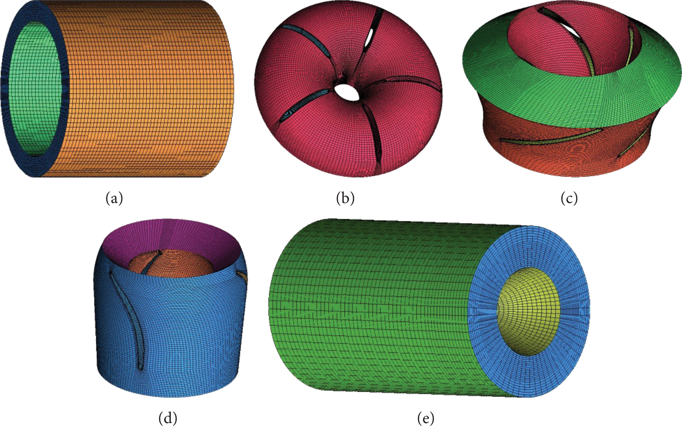
Five zones of the whole computational domain including (a) inlet pipe, (b) inducer, (c) impeller, (d) exit guide vane, and (e) outlet pipe.

Figure 3:

One quarter of the impeller.

Figure 4:

Sketch of the pump structured mesh.

During creating the mesh system, particular care has been taken in order to ensure a sufficient resolution along the blades, hub, and shroud as well as across the blade leading and trailing edges so that relatively fine grids are used near those locations. Due to strong variations in velocities near the solid wall areas, it is important to have sufficient amount of points inside the boundary layer to properly capture those large velocity gradients in the numerical simulations. The wall variable y⁺ varies between 0 and 1 for the utilized SST k-ω turbulence model (which will be introduced in detail later). To estimate y_wall as a function of a desired y⁺ value, a truncated series solution of the Blasius equation [14] is used:

y_{wall} = 6 {(\frac{U_{ref}}{ν})}^{- 7 / 8} {(\frac{L_{ref}}{2})}^{1 / 8} y^{+},

(1)

where U_ref can be taken as the mean velocity at the inlet and the reference length, L_ref, is the distance between hub and shroud curves that exist at the upstream of the first row of blade. This is an approximation, of course, since the thickness of boundary layers will vary widely within the computational domain. It is only necessary to place y⁺ within a specified range instead of at a certain value. The range of y⁺ = 0∼1 indicates that the near-wall nodes are within the laminar sublayer. Away from the solid wall boundary, the grid is stretched, which is a good compromise between the mesh points and the computational cost.

The resulting grid size used during the numerical simulations is determined after a grid independence analysis on the total head, with simulations carried out in the steady regime. The result of grid independence analysis is shown in Figure 5. It can be seen that when the mesh number is larger than 1.35 × 10⁶ cells the total head keeps almost the same. Finally, approximately 1.35 × 10⁶ cells are used for the following numerical simulations, which assure independent numerical results on the grid size.

Figure 5:

The simulated total head versus grid number.

2.3. Boundary Conditions

As inflow condition, mass flow rates associated with the targets for the simulations are specified. The simulated case is for an inlet flow rate Q_m = 305 kg/s, head H = 29.5 m, and rotating speed n = 2970 rpm. The direction of the absolute velocity vector is axially imposed at the inlet pipe. The inlet pipe at the upstream of the impeller is long enough to develop a full velocity profile before the flow enters the impeller. In the real situation, at the front of the impeller there are nonnegligible radial velocities that are important for the flow field in the impeller. However, due to the difficulties of setting up realistic turbulent inflow conditions, only the mass flow rate and the direction of the velocity are imposed. It is only expected here that the turbulent flow state can be fully developed by the interactions of flow with the solid wall. Therefore, in this context, the development of the turbulent structures may require an excessive length of the inlet section. Lund [15] provided an overview of inflow generation techniques.

The outlet is set as outflow boundary condition in the ANSYS CFX. The no-slip condition for the boundary layers is imposed over walls. Due to the rotation of impeller, two interfaces between the rotor and stator are formed, one of which is between the inducer and the impeller, and the other is between the impeller and the exit guide vane.

2.4. Governing Equations

The unsteady incompressible Reynolds-averaged Navier-Stokes (RANS) equations are solved for the flow passing through the axial-flow pump. The basic equations in a manner of RANS are the following continuity and momentum equations, respectively:

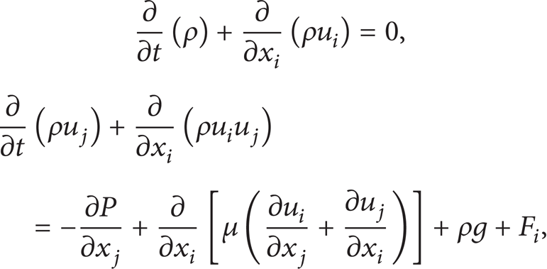
\begin{matrix} \frac{\partial}{\partial t} (ρ) + \frac{\partial}{\partial x_{i}} (ρ u_{i}) = 0, \\ \frac{\partial}{\partial t} (ρ u_{j}) + \frac{\partial}{\partial x_{i}} (ρ u_{i} u_{j}) = - \frac{\partial P}{\partial x_{j}} + \frac{\partial}{\partial x_{i}} [μ (\frac{\partial u_{i}}{\partial x_{j}} + \frac{\partial u_{j}}{\partial x_{i}})] + ρ g + F_{i}, \end{matrix}

(2)

where u is velocity vector, P is pressure, ρ and μ_m are density and dynamic viscosity of the simulated fluid, F_i is body force, and g is gravitational acceleration.

2.5. SST k-ω Turbulence Model

The unsteady flow was simulated using the shear stress transport (SST) k-ω model. The use of a k-ω formulation in the inner parts of the boundary layer makes the SST k-ω turbulence model directly usable all the way down to the wall through the viscous sublayer. Hence the SST k-ω model can be used as a low-Reynolds-number turbulence model without any extra damping functions [16]. The SST k-ω formulation also switches to k-ε behavior in the free-stream and thereby avoids the common k-ω problem where the model is too sensitive to the inlet free-stream turbulence properties. The SST k-ω model does produce a bit too large turbulence levels in regions with large normal strain, like stagnation regions and regions with strong acceleration, but this tendency is much less pronounced than that with a normal k-ε model. The transport equations for k and ω are as follows:

\begin{matrix} \frac{\partial (ρ k)}{\partial t} + \frac{\partial (ρ U_{j} k)}{\partial x_{j}} = \frac{\partial}{\partial x_{j}} [(μ + \frac{μ_{t}}{σ_{k}}) \frac{\partial k}{\partial x_{j}}] + P_{k} - β^{'} ρ k ω, \\ \frac{\partial (ρ ω)}{\partial t} + \frac{\partial (ρ U_{j} ω)}{\partial x_{j}} = \frac{\partial}{\partial x_{j}} [(μ + \frac{μ_{t}}{σ_{ω 1}}) \frac{\partial ω}{\partial x_{j}}] + (1 - F_{1}) 2 ρ \frac{1}{σ_{ω 2} ω} \frac{\partial k}{\partial x_{j}} \frac{\partial ω}{\partial x_{j}} + α_{1} \frac{ω}{k} P_{k} - β ρ k ω^{2}, \\ F_{1} = \tanh (ar g_{1}^{4}) \\ ar g_{1} = \min (\max (\frac{\sqrt{k}}{β^{'} ω y}, \frac{500 ν}{y^{2} ω}), \frac{4 ρ k}{C D_{k ω} σ_{ω 2} y^{2}}) \\ {C D}_{k ω} = \max (2 ρ \frac{1}{σ_{ω 2} ω} \frac{\partial k}{\partial x_{j}} \frac{\partial ω}{\partial x_{j}}, 1.0 \times 1 0^{- 10}) \\ μ_{t} = \frac{ρ α_{2} k}{\max (α_{2} ω, S F_{2})} \\ F_{2} = \tanh (ar g_{2}^{2}) \\ ar g_{2} = \max (\frac{2 \sqrt{k}}{β^{'} ω y}, \frac{500 ν}{y^{2} ω}) . \end{matrix}

(3)

If Φ₁, Φ₂, and Φ₃ stand for k-ω turbulence model, k-ε turbulence model, and SST turbulence model, respectively, then Φ₃ = F₁Φ₁ + (1-F₁)Φ₂. In the above equations, y is the distance from the wall, ν is kinematic viscosity of the working fluid, P_k is the production rate of turbulence, and S is the strain rate tensor.

2.6. Numerical Methods

The numerical simulations of the turbulent velocity field and pressure field in the model axial-flow water pump are carried out using a commercial CFD code, ANSYS CFX. The finite volume method is used for the discretization of governing equations (continuity equation and momentum equation) in the space region.

In the steady calculations, based on the so-called multiple reference frame model, the inlet pipe, outlet pipe, inducer, and exit guide vane are set in stationary frame, while the impeller is set in rotary frame. The unsteady simulation is then initialized from the solution of a steady calculation, whereby it is not performed until the steady convergence is reached. For the unsteady calculation, the sliding mesh technique is applied to simulate the rotor-stator interaction. The interfaces between two stationary components and rotary and stationary components are set as general grid interface and rotor/stator interface, respectively. Advection scheme is set to high resolution, and turbulence numeric is first order. The criterion for convergence is considered to be 10⁻⁴, allowing an optimal number of iterations for each time step. The time step is the time of the rotator passing one degree (5.6 × 10⁻⁵ s).

3. Results and Discussions

The total head predicted by SST k-ω turbulence model is slightly less than the designed value, with discrepancy of only 3.4%. From this point of view, we can conclude that the rotating turbulent flow inside the simulated axial-flow water pump obtained with SST k-ω model is credible, and it can be used to analyze the characteristics of the internal pressure field and velocity field.

3.1. Analysis on Velocity Field

Figure 6 is an overview of the streamline inside the axial pump. It can be seen that the flow in the inlet pipe to inducer is still smooth, which proves the necessity of an extension of the inlet pipe. When the liquid flows to the impeller, it begins to rotate with the blade and the magnitude of the velocity increases. And then the velocity begins to decrease and becomes less disordered when passing through the exit guide vane.

Figure 6:

Streamline inside the axial pump.

The stagger angle of the impeller blades is high and it is not constant over the span of the leading edge so that the incidence at the leading edge of the impeller is not the same over the full span. Figure 7 plots the velocity vector distributions at the leading edge of the impeller near the hub (span = 0.1), midspan (span = 0.5), and near shroud (span = 0.9). Comparing the incidence at midspan (Figure 7(b)) with that near the shroud (Figure 7(c)), it is seen that there is little difference between them. Near the hub (Figure 7(a)), where the blade angle and the thickness of the blade are different, however, there is a completely different image. The incidence is very high and a recirculation region at the suction side exits near the leading edge of the impeller. On the other hand, a very different pattern shows up on the pressure surface. A radial outward flow exists, which initiates the flow from the pressure side to the suction side through the tip leakage, as shown in Figure 8 for the streamline distributions. In addition, from hub to shroud, the velocity increases and tends to be smoothly distributed.

Figure 7:

Flow directions at the leading edge at different spans of impeller. (a) Span = 0.1, (b) span = 0.5, and (c) span = 0.9.

Figure 8:

Streamline at different spans of impeller. (a) Span = 0.1, (b) span = 0.5, and (c) span = 0.9.

The flow field in the impeller region at three different spans, as plotted in Figure 9, shows that the velocity is higher at the suction side than that at the pressure side. A minimum value of the velocity is observed at the suction side near the leading edge, which is increased towards the trailing edge. At the pressure side, the velocity has a higher value near the leading edge of the impeller, which firstly decreases and then increases towards the trailing edge. The high value at the leading edge is due to the high flow incidence. From hub to shroud, the low velocity region near the leading edge decreases in size, which means that the influence of the high flow incidence decreases gradually.

Figure 9:

Contour of velocity field at different spans of impeller. (a) Span = 0.1, (b) span = 0.5, and (c) span = 0.9.

Considering that “no-slip wall” boundary condition is employed, velocity is zero on the blade surface. Figure 10 uses streamlines to show the flow pattern near the pressure side (a) and suction side (b) of the impeller. The surface flow patterns on the suction surface (Figure 10(b)) show a two-dimensional flow feature. Again, as shown in Figure 8, one very different pattern is shown up on the pressure surface: a radial outward flow exists, indicating a flow from the hub to the shroud. Detailed inspection of Figure 10 demonstrates that stagnation lines exist and a small reverse flow is generated at the leading edge.

Figure 10:

Streamlines near the pressure side (a) and suction side (b) of the impeller.

The streamlines in exit guide vane are more irregular. There exist apparent vortex structures, as shown in Figures 11 and 12. The vortex structures are distributed mainly around the suction side, and the size of the vortex structures decreases from hub to shroud. At one circle the configuration of vortex structure is different due to the affection from upstream of impeller. And still, the magnitude of the velocity increases from hub to shroud.

Figure 11:

Streamlines at different spans of exit guide vane. (a) Span = 0.1, (b) span = 0.5, and (c) span = 0.9.

Figure 12:

Evolution of streamlines at different spans of exit guide vane in one circle.

Figures 13 and 14 are extracted turbulent vortex structures in the exit guide vane by means of Q-method [17]. Here Q = 156210 s⁻². It is clear that the vortex structure is vortex tube, and it varies in one circle. From Figure 14 we can see that the vortex tube is generated from the suction side of the blade and gradually separates from it. Suffering from the impact of the water from upstream, there exist almost no vortex structures near the pressure side of the blade.

Figure 13:

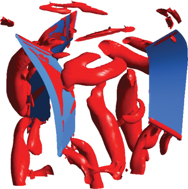
Extracted turbulent vortex structures in the exit guide vane by means of Q-method.

Figure 14:

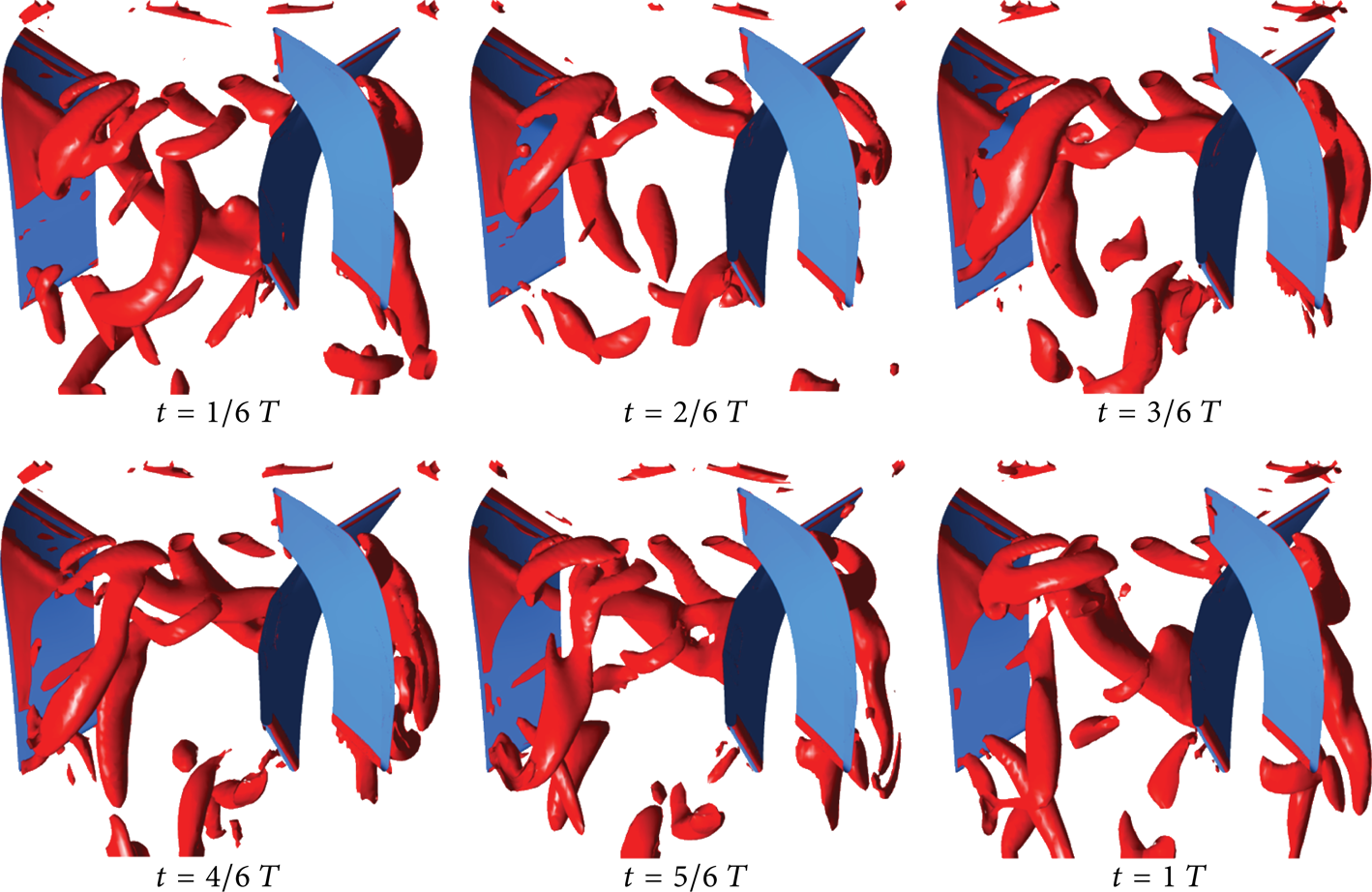
Extracted turbulent vortex structures in the exit guide vane in one circle.

3.2. Analysis on Pressure Field

The energy from the impeller is converted into pressure by applying the angular momentum to the constant mass flow of liquid going through the impeller blade. The increase of pressure in the rotor passage is very clear in the meridional view of pressure field (Figure 15) and overview of the pressure inside the axial-flow pump (Figure 16), which describes the energetic transmission happening in the passageway.

Figure 15:

Pressure of the axial-flow pump in view of meridional section.

Figure 16:

Sketch pressure of the axial-flow pump.

Figure 17 demonstrates the contour of the pressure field in the middle cross section of the impeller region in one circle. Notwithstanding that the blade position differs with the rotation, the pressure distribution is all the same at each moment as shown. Figure 18 illustrates the contour of the pressure field in different cross sections of the impeller region. It can be seen that pressure increases from the suction side to the pressure side and distributes in a striped style in the cross section near the leading edge (Figure 18(a)) and middle cross section (Figure 18(b)). In the cross section near the trailing edge (Figure 18(c)), the pressure is not as regular as that in Figures 18(a) and 18(b), where the pressure increases from hub to shroud.

Figure 17:

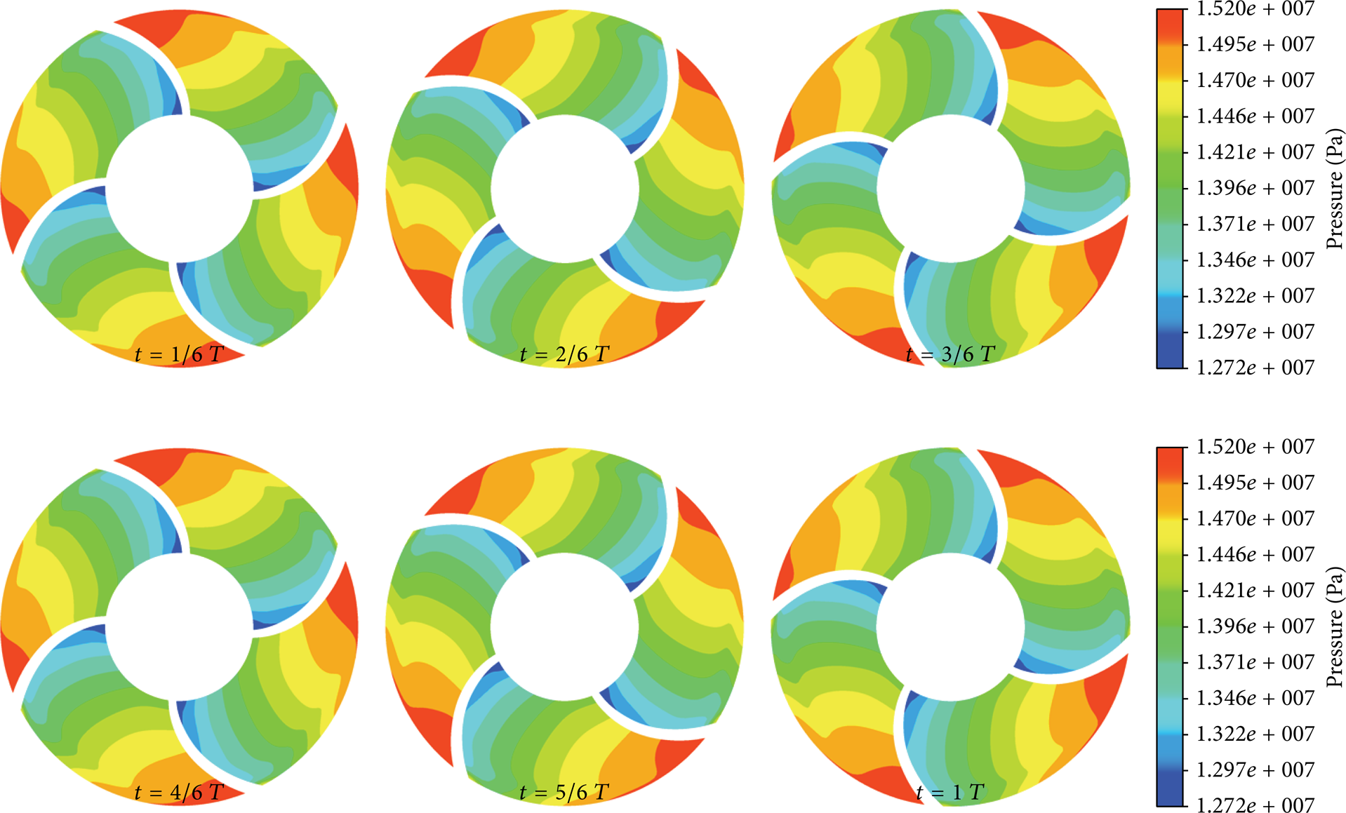
Contour of the pressure field in middle cross section of the impeller region in one circle.

Figure 18:

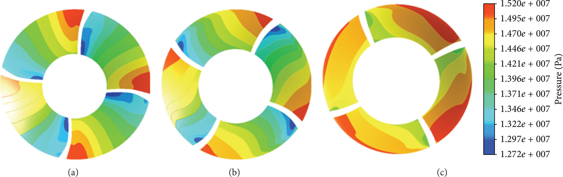
Contours of pressure field of different cross sections: (a) near the leading edge, (b) middle cross section, and (c) near the trailing edge.

Figure 19 plots the pressure distributions on the blades of the impeller at different spans. It can be seen that the pressure on suction side of the impeller increases from the leading edge to the trailing edge. At the pressure side of the impeller, the pressure is almost constant for all span positions, except that near the leading edge, where the pressure is very high because of the high flow incidence. At the suction side of the leading edge, it creates a very low pressure. At the trailing edge, the pressures at the pressure side and the suction side decrease due to the acceleration of the flow. Figure 20 plots the contours of pressures at different spans, which show the pressure distributions more visually.

Figure 19:

Pressure distributions at different spans. (a) Span = 0.1, (b) span = 0.5, and (c) span = 0.9.

Figure 20:

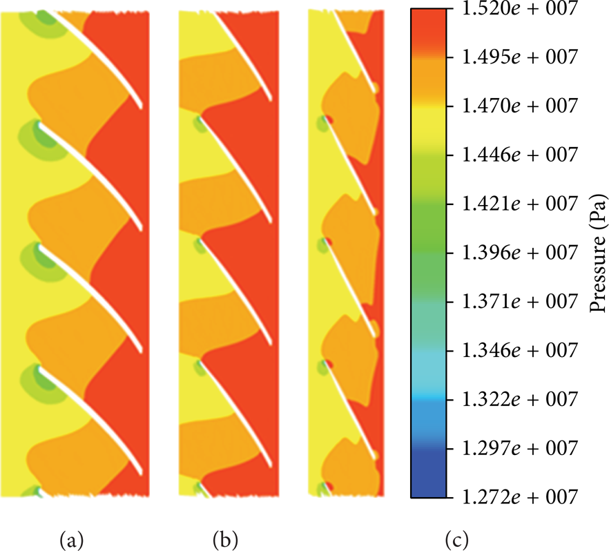
Contours of pressure fields at different spans. (a) Span = 0.1, (b) span = 0.5, and (c) span = 0.9.

Figure 21 demonstrates the contours of pressure fields at different spans of the exit guide vane. From hub to shroud, the pressure decreases gradually. There exist distinct low pressure areas near the leading edge in the suction side and near the trailing edge in the pressure side. Besides, due to the rotation of impeller and interaction between the impeller and exit guide vane, the pressure distribution in this zone is not as regular as in impeller zone.

Figure 21:

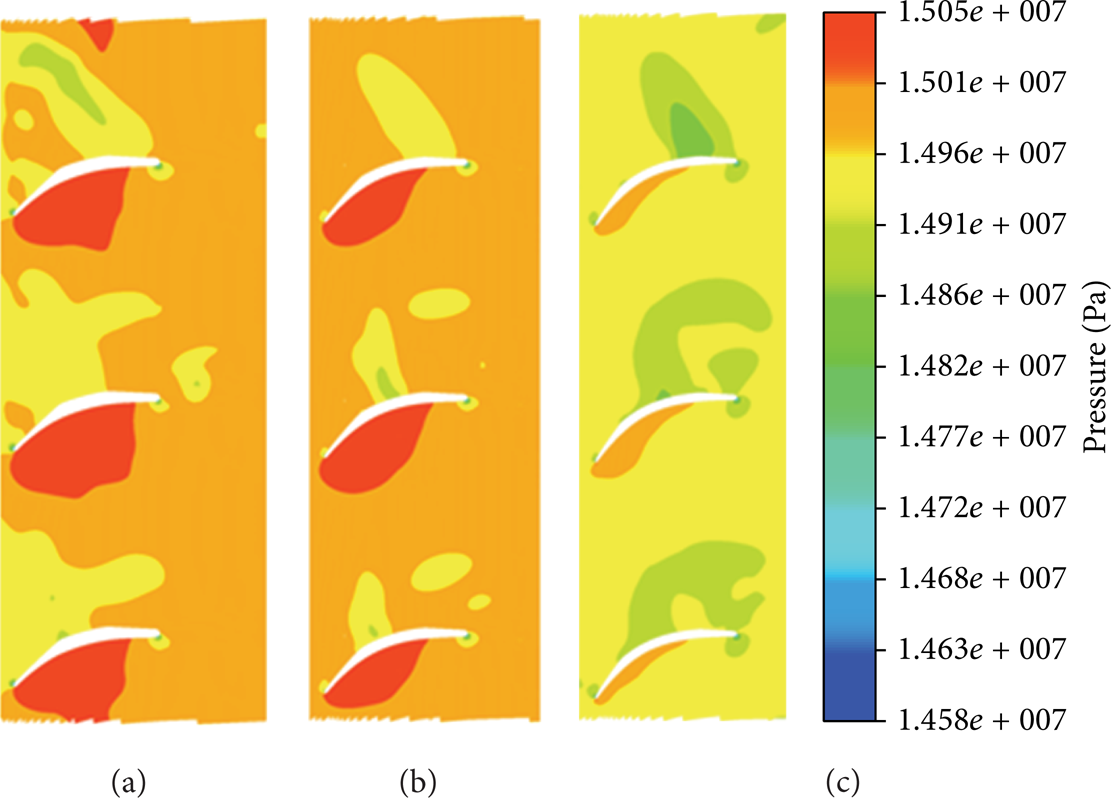
Contours of pressure fields at different spans of exit guide vane. (a) Span = 0.1, (b) span = 0.5, and (c) span = 0.9.

4. Concluding Remarks

Unsteady numerical simulations of the rotating turbulent flow in an axial-flow water pump have been carried out based on the RANS method and SST k-ω turbulence model. The presently established CFD numerical simulation procedure realized obtaining thorough information of the 3D complex flow field in the investigated model axial-flow water pump. All of the typical characteristics of the velocity field and pressure field have been successfully captured, which mainly include higher velocity at the suction side than that at the pressure side of the impeller, high incidence and appearance of a recirculation region at the suction side near the leading edge of impeller, increase of pressure from the suction side to the pressure side and a striped-style pressure distribution in the cross section, the pressure on suction side of the impeller which increases from the leading edge to the trailing edge, decrease of pressure at the trailing edge due to the acceleration of the flow, and existence of many turbulent coherent vortex structures in the impeller and exit guide vane regions. Therefore, the presently demonstrated numerical simulation procedure is of particular reference value to the related community and the obtained numerical simulation results can be used for further optimal design of the axial-flow water pump.

Conflict of Interests

The authors declare that there is no conflict of interests regarding the publication of this paper.

References

Zierke

W. C.

Straka

W. A.

, and Taylor

P. D.

, “Experimental investigation of the flow through an axial-flow pump,” Journal of Fluids Engineering, vol. 117, no. 3, pp. 485–490, 1995.

Zierke

W. C.

Farrell

K. J.

, and Straka

W. A.

, “Measurements of the tip clearance flow for a high-Reynolds-number axial flow rotor,” ASME Journal of Tubomachinery, vol. 117, no. 4, pp. 522–532, 1995.

Farrell

K. J.

, An investigation of end-wall vortex cavitation in a high Reynolds number axial-flow pump [M.S. thesis], Pennsylvania State University, Philadelphia, Pa, USA, 1989.

Alpan

and Peng

W. W.

, “Suction reverse flow in an axial-flow pump,” Journal of Fluids Engineering, Transactions of the ASME, vol. 113, no. 1, pp. 90–97, 1991.

Mostafa

N. H.

and Boraey

M. A.

, “Numerical and experimental investigation of cavitation in axial pumps,” in Proceedings of the 18th International Water Technology Conference, pp. 553–564, Sharm El-Sheikh, Egypt, 2007.

Furukawa

Shigemitsu

, and Watanabe

, “Performance test and flow measurement of contra-rotating axial flow pump,” Journal of Thermal Science, vol. 16, no. 1, pp. 7–13, 2007.

Zhang

Shi

Chen

, and Guan

, “Unsteady flow analysis and experimental investigation of axial-flow pump,” Journal of Hydrodynamics, vol. 22, no. 1, pp. 35–43, 2010.

Cao

Watanabe

Imanishi

Yoshimura

, and Furukawa

, “Experimental analysis of flow structure in contra-rotating axial flow pump designed with different rotational speed concept,” Journal of Thermal Science, vol. 22, no. 4, pp. 345–351, 2013.

and Wang

, “Numerical investigation of performance of an axial-flow pump with inducer,” Journal of Hydrodynamics, vol. 19, no. 6, pp. 705–711, 2007.

10.

Qian

Wang

Huai

, and Lee

, “Numerical simulation of water flow in an axial flow pump with adjustable guide vanes,” Journal of Mechanical Science and Technology, vol. 24, no. 4, pp. 971–976, 2010.

11.

Zhang

Pan

Shao

, and Wang

, “Numerical investigation of blade dynamic characteristics in an axial flow pump,” Thermal Science, vol. 17, no. 5, pp. 1511–1514, 2013.

12.

Zhang

Pan

Shi

, and Shao

, “Study on tip leakage vortex in an axial flow pump based on modified shear stress transport k-ω turbulence model,” Thermal Science, vol. 17, no. 5, pp. 1551–1555, 2013.

13.

Shuai

Z.-J.

W.-Y.

Zhang

X.-Y.

Jiang

C.-X.

, and Li

F.-C.

, “Numerical study on the characteristics of pressure fluctuations in an axial-flow water pump,” Advances in Mechanical Engineering, vol. 2014, Article ID 565061, 7 pages, 2014.

14.

Hinze

J. O.

, Turbulence: An Introduction to Its Mechanism and Theory, Mcgraw-Hill, New York, NY, USA, 1959.

15.

Lund

S. T.

, “Generation of turbulent inflow data for spatially-developing boundary layer simulations,” Journal of Computational Physics, vol. 140, no. 2, pp. 233–258, 1998.

16.

Menter

F. R.

, “Two-equation eddy-viscosity turbulence models for engineering applications,” AIAA journal, vol. 32, no. 8, pp. 1598–1605, 1994.

17.

Zhong

Huang

T. S.

, and Adrian

R. J.

, “Extracting 3D vortices in turbulent fluid flow,” IEEE Transactions on Pattern Analysis and Machine Intelligence, vol. 20, no. 2, pp. 193–199, 1998.

CFD Numerical Simulation of the Complex Turbulent Flow Field in an Axial-Flow Water Pump

Abstract

1. Introduction

2. Numerical Simulation Procedures

2.1. Computational Domain

2.2. Mesh Generation

2.3. Boundary Conditions

2.4. Governing Equations

2.5. SST k-ω Turbulence Model

2.6. Numerical Methods

3. Results and Discussions

3.1. Analysis on Velocity Field

3.2. Analysis on Pressure Field

4. Concluding Remarks

Conflict of Interests

References