Sage Journals: Discover world-class research

Abstract

In wireless sensor networks (WSNs), aggregator nodes perform the data aggregation process. Thus, careful selection of the aggregator nodes is needed to reduce network traffic in data aggregation process and prolong overall lifetime of the network. In this paper, we formulate selection process of the aggregator nodes as a top-k query problem. To answer the top-k queries efficiently in the large-scale WSNs, building and using the indexes are important. Thus, we propose an efficient index building algorithm for selection of aggregator nodes, called the Approximate Convex Hull Index (simply, aCH-Index). The main idea of our approach is to construct a convex hull over the sensor nodes in the WSNs, which enables speeding up the extraction of a set of sensor nodes that are potential candidates to become an aggregator node. In order to do so, the aCH-Index computes the skyline over the entire set of the sensor nodes, partitions the region into multiple subregions to reduce the computing time of convex hull in all origins, and then computes the convex hull in each subregion. Through the experiments with synthetic data, we show that aCH-Index outperforms the existing methods.

1. Introduction

A wireless sensor network (WSN) is a self-organized network composed of a large number of sensor nodes that interact with physical world [1, 2]. In a typical WSN, the sensor nodes have limited resources such as battery power, computing capability, and memory [3]. The data aggregation is the mechanisms to effectively use the limited resources in WSNs. In WSNs, the aggregator nodes perform the data aggregation process. Thus, careful selection of aggregator nodes is needed to reduce the network traffic in data aggregation process and prolong overall lifetime of the network [4]. However, network conditions change often because of resources sharing, computation load, and congestion on network nodes and links. These circumstances make the selection of the aggregator nodes difficult [5, 6].

In this paper, we formulate the selection process of aggregator nodes as a top-k query problem. There has been continuous interest in top-k query processing in database field. To answer the top-k queries efficiently in large databases, building and using the indexes are important. The layer-based methods are well-known techniques to answer top-k queries efficiently that use convex hull or skyline [7] to construct an index. A convex hull is the boundary of the smallest convex region of a set of points in space and the vertices are the subset of points on the boundary [8]. Intuitively, the convex hull is obtained by covering the point set. The convex hull can be expressed based on all attributes in the databases. It constructs the database as a layer list, where the ith layer includes the potential objects that can be the top-i answer. In other words, convex hull answers top-k queries by reading at most k layers from the layer list. However, the convex hull has problems of high time complexity and large memory usage, because it should maintain the information of all facets and calculate whether or not an object is inside of the particular facet [9]. On the other hand, the skyline can find the skyline points quickly, but its layer size can be large in high-dimensional databases [10].

In this paper, we propose an efficient index building algorithm for selection of aggregator nodes. Specifically, we propose a new convex hull method, called the Approximate Convex Hull Index (simply, aCH-Index), that can reduce the network traffic in selection of aggregator nodes in WSNs. The main idea of our approach is to construct a convex hull over the sensor nodes in the WSNs, which enables speeding up the extraction of a set of sensor nodes that are potential candidates to become an aggregator node. To do so, the aCH-Index computes the skyline over the entire set of the sensor nodes and partitions the region into multiple subregions to reduce the computing time of convex hull in all origins, and then computes the convex hull in each subregion.

More precisely, the contributions we make in this paper are as follows. (i)

We propose the aCH-Index that can reduce the number of candidate sensor nodes without false dismissal. The aCH-Index essentially combines aspects of a number of the established algorithms and reduces the computing time.

(ii)

Through the experiments with synthetic data, we show that the aCH-Index outperforms the existing methods.

The rest of this paper is organized as follows. Section 2 describes existing research related to this paper. Section 3 formally defines the problem. Section 4 introduces the proposed method. Section 5 presents the results of performance evaluation. Section 6 summarizes and concludes the paper.

2. Related Work

In this section, we discuss the existing work for answering top-k queries efficiently and top-k query processing in WSNs.

2.1. Indexing Algorithms for Top-k Query

In this section, we present the existing indexing algorithms for answering top-k query. There have been a number of index building methods proposed to answer top-k queries by accessing only a subset of the databases. The methods to construct an index using the convex hull or skyline are well known. We discuss the convex hull algorithms in Section 2.1.1 and skyline algorithms in Section 2.1.2.

2.1.1. Convex Hull Algorithms

The representative methods that use the convex hull are Onion [8] and HL-index (Hybrid-Layer Index) [11]. Onion constructs an index by making layers with the vertices of the convex hull over the objects in the multidimensional space. That is, it creates the first layer with the convex hull vertices over the all objects and then creates the second layer with the convex hull vertices over the remaining objects, and so on. Finally, the set of layers becomes the layer list. It is shown that Onion answers top-k queries by reading at most k layers starting from the outmost layer.

Onion is capable of answering a query with an arbitrary (monotone or nonmonotone) linear function because of the geometrical properties of the convex hull [12]. On the other hand, it takes a long time for Onion to compute convex hull. Because when new object is added, Onion should calculate whether new object is included in the convex hull or not. And it uses much memory to maintain the information needed in computing process [13].

HL-index constructs a layer list with the convex hull as Onion does and then constructs sorted lists in the ascending or descending order based on each attribute value of the objects in each layer. However, since HL-index constructs a layer lists as Onion does, the problems of high computing time and large memory usage still exist.

2.1.2. Skyline Algorithms

The representative methods that use skyline are BNL (Block Nested Loops) [7], SFS (Soft Filter Skyline) [14], and LESS (Linear Elimination Sort for Skyline) [15]. BNL sequentially reads the input relation and saves in a window w. When an object o is read, it is compared to objects in w. If an object in w dominates o, BNL eliminates o. Otherwise, if o dominates some objects in w, these are deleted from w and o is added to w [7]. The SFS algorithm [14] improves over BNL by presorting the input relation according to the entropy value of object. LESS is an improvement of SFS that essentially combines aspects of a number of the established algorithms [15]. LESS discards some dominated objects earlier; thus this has the advantage of reducing the number of pairwise comparisons between the objects more than that SFS has. However, the number of comparisons is still large.

The partitioning technique is also used in skyline algorithms. Vlachou et al. [16] proposed the angle-based partitioning technique for constructing skyline. PPPS (Plane-Project-Parallel Skyline) is proposed in [17], which makes a hyperplane by projecting the data objects first and then constructs skyline by partitioning the hyperplane.

2.2. Top-k Query Processing in WSN

In this section, we introduce top-k query processing methods in WSN.

The representative method for data aggregation in WSN is TAG (Tiny Aggregation Service) [8] and PANEL (Position-based Aggregator Node Election). TAG is a tree-based data aggregation protocol that builds a routing tree in top-down manner for sending data to the top sensor nodes. PANEL is a cluster-based data aggregation protocol that uses the geographical position information of the sensor nodes in order to select an aggregator node.

Nasridinov et al. [4, 18] proposed an efficient aggregator node selection method. Similar to our method, the authors formulate the selection process of aggregator node as a top-k query problem and solve it by using a modified Sort-Filter-Skyline (SFS) algorithm. The main idea of the proposed method is to immediately perform a skyline query on the sensor nodes in the WSN, which enables extracting a set of sensor nodes that are potential candidates to become an aggregator node.

3. Problem Definition

In this section, we formally define top-k queries focused in this paper, and the properties that our layering method should have. A target relation R has d attributes, $A_{1}, A_{2}, \dots, A_{d}$ of real values, and the cardinality of R is $C {8,12,16,25}$ . Every object in R can be considered as a point in the d-dimensional space ${[0.0,1.0]}^{d}$ . Hereafter, we call the space ${[0.0,1.0]}^{d}$ as the region and refer to an object o in the region [11, 19]. To maintain generality, we assume that we are searching the objects that have lowest value in the rest of this paper.

A top-k query Q is defined as a pair $f (o)$ and k, where $f (o)$ is a linear scoring function such that $\sum_{i = 0}^{d} w [i] * o [i]$ , where $o [i]$ is the ith attribute value of o and $w [i]$ is the weight of the ith attribute. The d-dimensional vector that has $w [i]$ as the ith element is called the preference vector [20], where d represents the number of attributes of o. We assume that $w [i]$ 's are normalized so that $\sum_{i = 0}^{d} w [i] = 1$ .

For processing these top-k queries, layer lists should satisfy optimally linearly ordered set property [8] in Definition 1 below. In other words, in the ith layer, there is at least one object, whose score for any weight $w [i]$ $(1 \leq i \leq d)$ is lower than or equal to those of all the objects in subsequent layer. Thus, top-k queries are answered by reading objects in at most k layers.

Definition 1 (optimally linearly ordered sets [8]).

A collection of sets $S = {S_{1}, S_{2}, \dots, S_{m}}$ , where each set consists of d-dimensional point objects, is optimally linearly ordered if and only if, given any d-dimensional vector p,

\begin{matrix} \exists x \in S_{i} s . t . \\ \forall y \in S_{i + j}, j > 0, p \dots x \leq p \cdot y, \end{matrix}

(1)

where

p \cdot x

represents the inner product of the two vectors p and x.

At “The Notations” section in the end of paper, we summarized notations that we use throughout this paper. The symbols that have not been introduced yet will be explained in Section 4.

4. The Approximate Convex Hull Index (aCH-Index)

In this section, we explain the proposed method, the Approximate Convex Hull Index (aCH-Index). The computing time of convex hull method becomes slow and memory usage becomes large as the dimension increases. The aCH-Index reduces the computing time and memory usage of convex hull by constructing skyline layer and partitioning the region. In Section 4.1, we give the overview of the aCH-Index. We explain each step of the aCH-Index in detail in Sections 4.2, 4.3, and 4.4. In Section 4.5, we explain an example of constructing the convex hull in WSNs.

4.1. Overview

The aCH-Index is constructed by three steps as shown in Figure 1: (a) skyline layering step, (b) partitioning step, and (c) computing step. For the convenience of the explanation, Figure 1 shows the process of constructing the first layer in two-dimensional region.

Figure 1

Overall process of constructing the aCH-Index in the two-dimensional region.

More precisely, in the skyline layering step, we compute the skyline over the entire set of the objects. By building the skyline layer in the first step, the aCH-Index will be able to get the result set without false dismissal. In Figure 1(a), the line composed of black points represents the skyline and the dotted line represents the skyline layer.

In the partitioning step, we can reduce the size of candidate objects once again by partitioning the skyline layer, obtained in the skyline layering step, into m subregions. We can get ${subregion}_{1}, {subregion}_{2}, \dots, {subregion}_{m}$ as shown in Figure 1(b) by partitioning the skyline layer.

In the computing step, we compute the convex hull over the skyline layer in each subregion m times. In Figure 1(c), the dotted line represents the first layer of the aCH-Index.

Algorithm 1 shows the Approximate Convex Hull Algorithm. The input to the Approximate Convex Hull Algorithm is the data objects in database (i.e., sensor nodes in WSNs), and the output is Approximate Convex Hull Index. In lines 1 to 3, we initialize an index and set the number of subregions and a virtual object. We first compute Skyline Layering Algorithm, which will be introduced in Section 4.2, in line 4. Next, in the second step, we partition skyline $SL$ into m subregions in line 5. In lines 6 to 14, we compute the convex hull and if the data objects are in convex hull, then we insert the objects to resulting index in line 12. Lines 15 to 21 describe the IsConvexhull function that computes the convex hull.

Algorithm 1: The Approximate Convex Hull Algorithm.

Input: Data Objects in Database $o [0, \dots, n]$

Output: Approximate Convex Hull Index aCH-Index

Algorithm:

(1) Initialize a Approximate Convex Hull Index aCH-Index.

(2) Set $m = 2^{\land} n$ . //the number of subregions.

(3) Set $v C$ as the virtual object with central value.

(4) Compute Skyline Layering Algorithm.

//Algorithm 2

(5) Partitions SL into m subregions using $v C$ .

(6) for $i = 0$ to m do

(7) for $j = 0$ to n do

(8) Convert $o [j]$ to $o^{'} [j]$ based on ith origin.

(9) end for

(10) for $j = 0$ to n do

(11) if IsConvexhull( $o^{'} [j]$ ) then

(12) Insert $o^{'} [j]$ to aCH-Index

(13) end for

(14) end for

(15) Function: IsConvexhull(Data object $o^{'}$ )

(16) Compute convex hull method

(17) if $o^{'}$ is convex hull then

(18) Set candidate = true.

(19) else

(20) Set candidate = false.

(21) return candidate;

4.2. Skyline Layering Step

The objects in the skyline layer are subsets of the convex hull objects. In this paper, we adopt the SFS algorithm [14] as a method of constructing the skyline, which presorts the input objects according to the entropy value of object. Equation (2) represents the entropy value of an object o on the region:

\begin{matrix} E (o) = \sum_{i = 1}^{d} \ln (o^{'} [i] + 1) . \end{matrix}

(2)

Here, $o^{'} [i]$ is the normalized value of the ith attribute. Intuitively, if an object has the smaller entropy value, the less likely the object is dominated by others [21].

Figure 2 shows the process of skyline layering step in the two-dimensional region. In Figure 2(a), the objects are presented in the two-dimensional region. In Figures 2(b) and 2(c), the line composed of black points represents the skyline in origins $O_{1}$ and $O_{2}$ . The aCH-Index computes the skyline in $O_{3}$ and $O_{4}$ in the same way as in origins $O_{1}$ and $O_{2}$ and then merges the skyline objects into skyline layer by avoiding redundancy. In Figure 2(d), the dotted line represents the resulting skyline layer.

Figure 2

The process of skyline layering in the two-dimensional region.

Algorithm 2 shows the Skyline Layering Algorithm. The input to the Skyline Layering Algorithm is data objects in database (i.e., sensor nodes in WSNs), and the output is a skyline layer. In lines 1 to 4, we initialize a skyline layer and set a number of origins and number of skyline. In lines 5 to 14, we construct skyline layer. First, we sort the data objects using entropy value in line 6. Lines 16 to 20 describe Sort function. In lines 7 to 13, we compute skyline in each origin. We compute the IsSkyline function in line 7. In lines 24 to 30, the IsSkyline function compares data object and skyline layer to figure out the dominating relationship between them. If data object dominates the skyline object, then we remove skyline object from $SL$ in lines 26 to 27. If data object and skyline object do not dominate each other, then algorithm sets the candidate parameter as true in lines 28 to 29. We insert data object if it is determined as a skyline in lines 9 to 12.

Algorithm 2: The Skyline Layering Algorithm.

Input: Data Objects in Database $o [0, \dots, n]$

Output: Skyline Layer SL

Algorithm:

(1) Initialize a Skyline Layer SL.

(2) Set $SL = φ$ .

(3) Set $c = 2^{\land} n$ . //the number of origins.

(4) Set $s = 0$ / //the number of skyline.

(5) for $i = 0$ to c do

(6) Sort(o).

(7) if IsSkyline( $o [i]$ ) then

(8) if $i = 0$ then

(9) Insert $o [i]$ to SL.

(10) $s = s + 1$ .

(11) else if $o [i]$ is not $\subset SL$ then

(12) Insert $o [i]$ to SL.

(13) $s = s + 1$ .

(14) end for

(15) return SL;

(16) Function: Sort(Data Objects $o []$ )

(17) for $i = 0$ to n do

(18) Calculate the entropy value of $o [i]$ .

(19) end for

(20) Sort data objects according to the entropy value.

(21) Function: IsSkyline(Data Object o)

(22) Set candidate = false;

(23) for $i = 0$ to s do

(24) if $SL [i]$ dominates o then

(25) break;

(26) if o dominates $SL [i]$ then

(27) Erase $SL [i]$ from SL.

(28) else

(29) Set candidate = true;

(30) end for

(31) return candidate;

4.3. Partitioning Step

In the partitioning step, we can reduce the number of candidate objects once again by partitioning the skyline layer, obtained in the skyline layering step, into m subregions. We partition the skyline layer because the number of skyline layer objects in each subregion is smaller than that of the entire skyline layer. We partition the region using $v C$ , which is a virtual object whose coordinate value of ith axis. We select the $v C$ as the center object in the region, where it has medium value between minimum and maximum values of each axis. We construct the skyline layer in first and then we partition the region. Otherwise, it may cause false dismissals.

4.4. Computing Step

In the computing step, we compute the convex hull over the skyline layer objects in each subregion m times to find the aCH-Index and then merge the results of each subregion. The layer size of the aCH-Index becomes larger than that of the convex hull, but computing time of the aCH-Index is faster. The aCH-Index also includes all objects of the convex hull.

4.5. Convex Hull in WSN

In this section, we explain an example of convex hull in WSN as the two-dimensional space using aCH-Index. Let us consider an example of an aggregator node selection in Figure 3. There are 12 sensor nodes, and they have two attributes such as computing capability and battery life. We first construct aCH-Index over the sensor nodes.

Figure 3

An example of aCH-Index on sensor nodes.

Figure 3 shows an example of convex hull sensor nodes that are represented as points in the two-dimensional space. The x-axis represents computing capability and y-axis represents battery life. As shown in Figure 3, we construct aCH-Index over the sensor nodes. The sensor nodes $SN 1$ , $SN 2$ , $SN 3$ , $SN 4$ , $SN 5$ , $SN 8$ , and $SN 9$ are included in the first layer and $SN 6$ , $SN 7$ , $SN 10$ , $SN 11$ , and $SN 12$ are included in the second layer.

Consider a top-1 query to find the aggregator node, which has the highest computing capability and battery life. The sensor node $SN 5$ is the top-1 result, when considering both of the attributes. Consider another top-1 query to find the aggregator sensor node, which has the highest battery life and the lowest computing capability. For this query, $SN 8$ is the top-1 result.

5. Performance Evaluation

We first explain the data and environment used in the experiment in Section 5.1. We then demonstrate the results of the experiments in Section 5.2.

5.1. Experimental Data and Environment

We perform experiments using a synthetic dataset. For the synthetic dataset, we generate uniform dataset (UNIFORM) by using the generator introduced by Bhaniramka et al. [22]. The dataset consists of four-, five-, and nine-dimensional dataset of 1 K, 10 K, and 100 K objects.

We compare the computing time and the $nER$ (normalized eliminating rate) of the aCH-Index with the existing method convex hull [23] (simply, CH). We use the wall clock time as the measure of the computing time. We compare the $nER$ , which measures how many useless objects are eliminated in the skyline layering step. For the $nER$ , we use the number of objects not contained in a layer of CH with the number of eliminated objects in the skyline layering step. The $nER$ is shown in

\begin{matrix} nER = \frac{{eliminated objects}}{{remaining objects}} . \end{matrix}

(3)

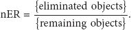
Here, {eliminated objects} is the objects filtered by the skyline layering step, and {remaining objects} is the objects not contained in the layer of the CH. To calculate the $nER$ of these methods on the CH, we have found the outmost layer of the aCH-Index and the CH.

We have implemented the aCH-Index and the convex hull using C++. To compute convex hull, we used the Qhull library [13]. To compute skylines, we used the SFS algorithm [14]. We conducted all the experiments on an Intel i5-760 quad core processor running at 2.80 GHz Linux PC with 16 GB of main memory.

5.2. Results of Experiments

We measure the $nER$ and the computing time of the aCH-Index and CH on the synthetic dataset while varying the number of objects N and the dimension d. For the experiments in this section, we use $d = 8$ and $N = 10$ K because of hardware limitation.

Experiment 1.

$nER$ as data size N and dimension d is varied.

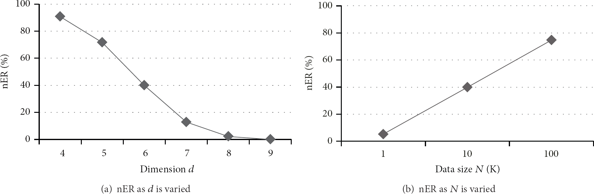
Figure 4(a) shows that the $nER$ of the aCH-Index as d is varied from 4 to 9. Figure 4(b) shows that the $nER$ of the aCH-Index as N is varied from 1 K to 100 K. The $nER$ of the aCH-Index decreases as dimension d increases, but the $nER$ of the aCH-Index increases as data size N increases. Thus, the number of eliminated objects decreases over high-dimensional dataset, but it will increase over the large dataset. In particular, with $N = 100$ K objects, the $nER$ still prunes about 74% tuples.

Figure 4

The comparison of the $nER$ as d and N is varied.

Experiment 2.

Computing time as dimension d is varied.

Figure 5 shows that the computing time of the aCH-Index and the CH as d is varied from 4 to 9. The aCH-Index improves by 7.97 times over the computing time of the CH on average. Especially the aCH-Index improves by 28.76 times over the computing time of the CH when d is 9. The difference of the computing time becomes big as dimension d increases.

Figure 5

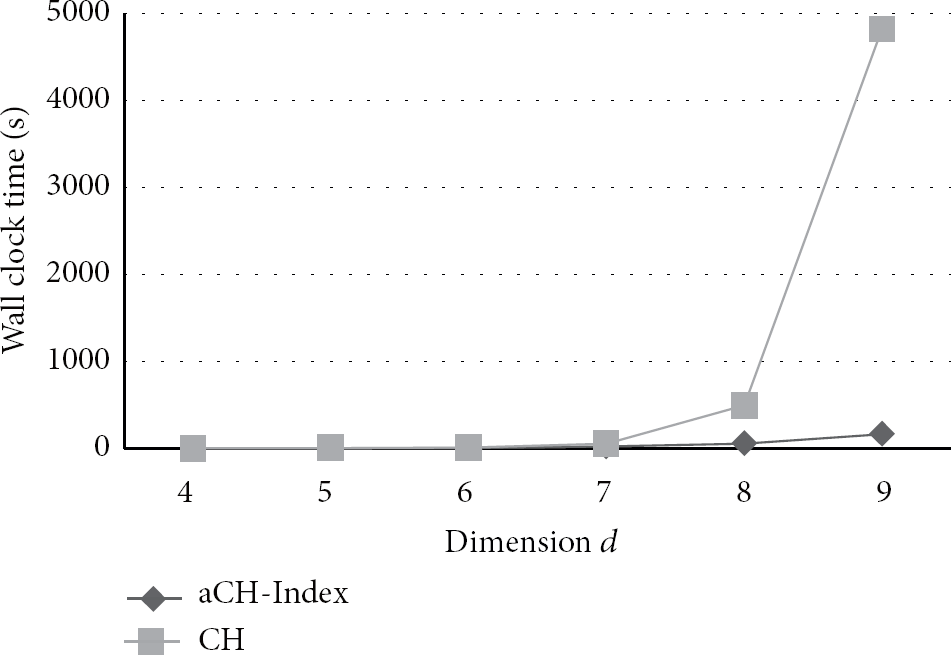
The comparison of the time as d is varied.

Experiment 3.

Computing time as data size N is varied.

Figure 6 shows that the computing time of the aCH-Index and the CH as N is varied from 1 K to 100 K. The computing time of the aCH-Index improves by 1.58–39.26 times over that of the CH.

Figure 6

The comparison of the time as N is varied.

6. Conclusion

In this paper, we have formulated the selection process of the aggregator nodes as a top-k query processing problem. In order to solve it, we have proposed an efficient index building algorithm for selection of aggregator nodes, called aCH-Index. Our approach selects a set of aggregator nodes according to their attributes, such as distance from the base station, power consumption, battery life, and communication cost. Thus, we can reduce large amounts of communication traffic by sending only the aggregated data through selected aggregator nodes, instead of individual sensor data, to the base station. We have performed experiments on a synthetic dataset by varying the data size and the dimension. Experimental results show that aCH-Index reduces the number of candidate objects and improves the computing time compared to the convex hull.

Footnotes

The Notations

Conflict of Interests

The authors declare that there is no conflict of interests regarding the publication of this paper.

Acknowledgment

This research was supported by Basic Science Research Program through the National Research Foundation of Korea (NRF) funded by the Ministry of Education, Science, and Technology (no. 20110002707).

References

Liu

Underground structure monitoring with wireless sensor networks

Proceedings of the 6th International Conference on Information Processing in Sensor Networks (IPSN ′07)

April 2007

Cambridge, Mass, USA

69 78

Dubey

Sahu

O. P.

Self-localized packet forwarding in wireless sensor networks

Journal of Information Processing 2013 9 3 477 488

10.3745/JIPS.2013.9.3.477

Lee

H. R.

Chung

K. Y.

Jhang

K. S.

A study of wireless sensor network routing protocols for maintenance access hatch condition surveillance

Journal of Information Processing Systems 2013 9 2 237 246

10.3745/JIPS.2013.9.2.237

Nasridinov

Ihm

S.-Y.

Park

Y.-H.

Skyline-based aggregator node selection in wireless sensor networks

International Journal of Distributed Sensor Networks 2013 2013 7

356194

10.1155/2013/356194

Park

Y.-H.

Whang

K. Y.

Lee

B. S.

Han

W. S.

Efficient evaluation of partial match queries for XML documents using information retrieval techniques

Proceedings of the 10th International Conference on Database Systems for Advanced Applications (DASFAA ′05)

April 2005

Beijing, China

95 112

Subhlok

Lieu

Lowekamp

Automatic node selection for high performance applications on networks

Proceedings of the 7th ACM SIGPLAN Symposium on Principles and Practice of Parallel Programming (PPoPP ′99)

May 1999

Atlanta, Ga, USA

163 172

2-s2.0-0032643892

Börzsönyi

Kossmann

Stocker

The skyline operator

Proceedings of the 17th International Conference on Data Engineering (ICDE ′01)

April 2001

Heidelberg, Germany

421 430

2-s2.0-0035008034

Chang

Y. C.

Bergman

Castelli

C. S.

M. L.

Smith

J. R.

The onion technique: indexing for linear optimization queries

Proceedings of the ACM SIGMOD International Conference on Management of Data (SIGMOD ′00)

May 2000

Dallas, Tex, USA

391 402

Barber

C. B.

Dobkin

D. P.

Huhdanpaa

The quickhull algorithm for convex hulls

ACM Transactions on Mathematical Software 1996 22 4 469 483

2-s2.0-0030381077

10.

Ihm

S.-Y.

Lee

K.-E.

Nasridinov

Heo

J.-S.

Park

Y.-H.

Approximate convex dkyline: a partitioned layer-based index for efficient processing top-k queries

Knowledge-Based Systems 2014

10.1016/j.knosys.2014.01.022

11.

Heo

J.-S.

Cho

Whang

K.-Y.

The hybrid-layer index: a synergic approach to answering top-k queries in arbitrary subspaces

Proceedings of the 26th IEEE International Conference on Data Engineering (ICDE ′10)

March 2010

Long Beach, Calif, USA

445 448

2-s2.0-77952750561

10.1109/ICDE.2010.5447908

12.

Gass

S. I.

Linear Programming: Method and Applications 1985

New York, NY, USA

Dover

13.

Adibi

Data mining: a captured wired traffic approach

International Journal of Advanced Science and Technology 2010 21 2 11 29

14.

Chomicki

Godfrey

Gryz

Liang

Skyline with presorting

Proceedings of the 19th International Conference on Data Engineering (ICDE ′03)

March 2003

Bangalore, India

717 719

2-s2.0-0344927722

10.1109/ICDE.2003.1260846

15.

Godfrey

Shipley

Gryz

Maximal vector computation in large data sets

Proceedings of the 31st International Conference on Very Large Data Bases (VLDB ′05)

September 2005

Trondheim, Norway

229 240

2-s2.0-33745601731

16.

Vlachou

Doulkeridis

Kotidis

Angle-based space partitioning for efficient parallel skyline computation

Proceedings of the ACM SIGMOD International Conference on Management of Data (SIGMOD ′08)

June 2008

Vancouver, Canada

227 238

2-s2.0-57149128192

10.1145/1376616.1376642

17.

Köhler

Yang

Zhou

Efficient parallel skyline processing using hyperplane projections

Proceedings of the ACM SIGMOD International Conference on Management of Data (SIGMOD ′11)

June 2011

Athens, Greece

85 94

2-s2.0-79959945239

10.1145/1989323.1989333

18.

Nasridinov

Jang

Park

Y.-H.

Partitioning-based selection of aggregator nodes in wireless sensor networks

Proceeding of the 8th International Conference on Ubiquitous Information Technologies and Applications (CUTE ′13)

December 2013

Danang, Vietnam

Springer

763 768

19.

Gope

Kehtarnavaz

Affine invariant comparison of point-sets using convex hulls and hausdorff distances

Pattern Recognition 2007 40 1 309 320

2-s2.0-33749426752

10.1016/j.patcog.2006.04.026

20.

Hristidis

Papakonstantinou

Algorithms and applications for answering ranked queries using ranked views

The VLDB Journal 2004 13 1 49 70

2-s2.0-0942279014

10.1007/s00778-003-0099-8

21.

Pei

Yuan

Lin

Jin

Ester

Liu

Wang

Tao

J. X.

Zhang

Towards multidimensional subspace skyline analysis

ACM Transactions on Database Systems 2006 31 4 1335 1381

2-s2.0-33846200457

10.1145/1189769.1189774

22.

Bhaniramka

Wenger

Crawfis

Isosurface construction in any dimension using convex hulls

IEEE Transactions on Visualization and Computer Graphics 2004 10 2 130 141

2-s2.0-1342324591

10.1109/TVCG.2004.1260765

23.

Bohm

Kriegel

Determining the convex hull in large multidimensional databases

Proceedings of the Data Warehousing and Knowledge Discovery (DaWaK ′01)

September 2001

Munich, Germany

294 306

An Efficient Index Building Algorithm for Selection of Aggregator Nodes in Wireless Sensor Networks

Abstract

1. Introduction

2. Related Work

2.1. Indexing Algorithms for Top-k Query

2.1.1. Convex Hull Algorithms

2.1.2. Skyline Algorithms

2.2. Top-k Query Processing in WSN

3. Problem Definition

Definition 1 (optimally linearly ordered sets [8]).

4. The Approximate Convex Hull Index (aCH-Index)

4.1. Overview

Algorithm 1: The Approximate Convex Hull Algorithm.

4.2. Skyline Layering Step

Algorithm 2: The Skyline Layering Algorithm.

4.3. Partitioning Step

4.4. Computing Step

4.5. Convex Hull in WSN

5. Performance Evaluation

5.1. Experimental Data and Environment

5.2. Results of Experiments

Experiment 1.

Experiment 2.

Experiment 3.

6. Conclusion

Footnotes

The Notations

Conflict of Interests

Acknowledgment

References