Sage Journals: Discover world-class research

Abstract

Data collection is an important procedure of ocean monitoring systems. Due to limited bandwidth and extreme high cost of satellite communication, the majority of data is unable to transmit via satellites. For the moment, there are no efficient data collection methods provided for data collection in underwater sensor networks. After collecting and analyzing GPS data of 40 ships for two months, we find the mobility pattern of ships. On the basis of the mobility pattern, we propose a new data collection strategy for underwater sensor networks through delay tolerant routing. Through simulations and real data analysis, we provide quantitative analysis of the proposed strategy, such as data collection ratio, complexity of the algorithm and energy consumption. Especially, the data collection ratio on real data analysis could reach 95%–100% in acceptable time, which is 30% more than the radio of the strategy that data stored as they come.

1. Introduction

The ocean has become one of the most important treasures of people's resources with the development of human society and also has significant impact on the change of global climate. Therefore, the research of the ocean has become one of the most important development strategies of the costal countries for many years. Long-term automatic monitoring is a common technique for the study of the ocean [1–3]. Due to the limited bandwidth and the extreme high cost of satellite communication, the majority of the data is unable to be transmited in real time. In this case, the traditional method is the local storage of the mass data and regular collection by special data mules after a long cycle interval [2–4] or using AUV as substitution for sensors [5–8]. However, these approaches not only reduce the efficiency due to difficulty in obtaining the real-time data but also significantly increase the cost.

To reduce the cost, delay tolerant network provides a by-product effective technical approach for data collection problem [9–11]. The designers use mobile devices which always travel between sources and destinations by the way, such as buses or robots, to deliver messages [9, 10, 12–14]. Motivated by this, we observe that many ships work on the ocean every day, and some of them may pass across the monitoring area. Taking advantage of these passing ships to help the data collection may be a feasible plan.

However, unlike the delay tolerant network on land, ocean delay tolerant network has different characteristics and some challenges are as follows. First, the ocean network usually adopts acoustic communications. Different from the terrestrial wireless communications, the acoustic communications have the properties of low bandwidth, high latency, and high error rate and are seriously affected by multipath transmission and Doppler effect [15–17]. The data transmission between ships and sensors is achieved by acoustic communications. Because the transmission rate of underwater sensors is very low and the traffic volume of ships is not as much as that of vehicles, increasing the average transmission efficiency is a more urgent problem of data collection. Second, the mobility patterns of ships and vehicles are different. The vehicle trace is strictly confined by roads [14, 18]. In other words, different vehicles have the same trace when they pass through the same road. However, there are no roads in the ocean like overland. We need to find the mobility pattern in the ocean which could support our work. Through this pattern, we may generate paths with different probabilities from large amounts of GPS data. Based on the different probabilities of the paths, we propose to design a strategy to allocate data to different sensors in the monitoring area. Third, there is no routing plan designed for data collection in ocean delay tolerant network. In order to increase the transmission efficiency and the data collection radio, we need to route data to the sensors which can easily communicate with ships. Many effective routing protocols have been designed for delay tolerant network [18–22]. However, some of them are designed for message delivery which cannot be adopted for massive data transmission because of the short interactive period, and others are context-related or probability-related routing plan which cannot realize the data routing of multipoint to paths with different probability. We need to design a routing plan which could distribute the data of the whole network to several paths with different probabilities and realize massive data transmission.

In order to investigate the mobility pattern of ships, we collect the trace data of 40 ships for two months (from 2011-07-01 to 2011-08-31). From these data as shown in Figure 1, we observe that the trace of ship is not regular as that of vehicle despite of the navigational aid equipped. Through analyzing the historical GPS data, we propose a new method to find out several approximately estimated paths of a monitoring area that the ships would pass through.

Figure 1

The traces of ships (from 2011-08-01 to 2011-08-06).

In this paper, we provide an efficient data collection strategy based on the mobility pattern of ships. To the best our knowledge, this is the first detailed, systematic data collection strategy in ocean monitoring field. And it is the first paper report on mobility pattern of ships with real data at this scale. We summarize the main contributions of this paper as follows. (1)

We propose an innovative method to generate estimated paths by summarizing the general rule from large amounts of ship traces collected by experiments. The estimated paths could be used in data allocation and data routing procedure.

(2)

We provide a routing plan of multipoints to paths of different probabilities. We transform the data routing problem to the assignment problem. Because of the specific characteristic of this assignment problem, in order to save computing resources, we design a greedy algorithm and its complexity is $O (n^{2})$ .

(3)

We design a data collection strategy to collect data from the sensors based on the mobility pattern of ships. In this system, we take advantage of the mobility pattern of ship which we have summarized and the routing plan we have provided to boost the speed of data collection by routing the data to the sensors near estimated paths.

(4)

We conduct extensive trace-driven experiments, and the experimental results show that the collection ratio of our strategy could reach 95%–100% in acceptable time, which is 30%–150% more than the radio of the strategy that data stored as they come.

The paper is organized as follows. In Section 2, we introduce the characteristics of ship traces and provide a method to generate the estimated paths of ships. The design of the data allocation strategy is described in Section 3. The data routing problem is discussed in Section 4. In Section 5, we provide the simulation with both simulated data and real data. We survey the related work in Section 6. Finally, conclusions are presented and suggestions are made for future research in Section 7.

2. Estimated Path Generation

In this section, we will discuss the mobility pattern of ships. Based on the pattern, we describe the definition of the distance between two curves and the method of estimated paths generation which can be used during data collection.

2.1. Trace Analysis

As we discussed in Section 1, the traces of ships have the specialty of no road confined. In order to find the mobility pattern of ships, we put our devices on 40 ships in The Yellow Sea for two months (from 2011-07-01 to 2011-08-31) to collect their GPS data.

Through analyzing the GPS data of ships, we preliminarily find that the sailing traces of the ships are regular as Figure 1 shows. The traces of different ships of same harbor sailing to one target are all different every time; however, these traces seem to be confined by an invisible boundary. Even if the traces are not like the vehicle's which can be confined by roads in tens of meters, but the underwater sensor's large communication range could tolerate the error of hundreds of meters.

As these similar traces are regular and confined within range, they could be treated as one trace just like the overland roads. Apparently, any of them could not represent for others. So, we provide a method which could fuse several paths from these historical traces which could summarize the general rule of these traces. Transmitting data to the sensors near these fusion paths could make the data collection work efficient, because these paths could roughly represent the ships’ sailing paths.

2.2. Distance between Two Curves

Before path fusion, we will introduce a new definition, the distance between two curves.

We assume that the distance between curves $a (r_{a})$ and $b (r_{b})$ is $d_{a b}$ . For every point $x_{a k} (k = 1,2, \dots, n, \dots)$ of $r_{a}$ , calculate the minimum distance $l_{a k} (k = 1,2, \dots, n, \dots)$ from $x_{a k}$ to $r_{b}$ . Similarly, we can work out every $l_{b k} (k = 1,2, \dots, n, \dots)$ of $r_{b}$ . The distance $d_{a b}$ between curves a and b is defined as follows:

\begin{matrix} d_{a b} = \max {l_{a 1}, l_{a 2}, \dots, l_{a n}, \dots, l_{b 1}, l_{b 2}, \dots, l_{b n}, \dots} . \end{matrix}

(1)

Figure 2 is the example of the distance between two curves. As shown in Figure 2, obviously, $l_{a i}$ is the maximum of ${l_{a 1}, l_{a 2}, \dots, l_{a n}, \dots, l_{b 1}, l_{b 2}, \dots, l_{b n}, \dots}$ . So, $l_{a i}$ is the distance between curves a and b.

Figure 2

The example of distance between curves a and b.

2.3. Path Fusion

The distance between two curves can effectively express the similarity of two curves. The shorter it is, the more similar they are. We can use this definition to support our path fusion(Algorithm 1).

Algorithm 1: Path fusion.

Input: Array of paths $p a t h [N]$ ;

Output: Fusion path set F;

sortDesc( $p a t h$ , $p a t h \cdot n e a r P a t h I d s \cdot l e n g t h$ );

for each $p a t h [i]$ do

$p a t h [i] \cdot i s F u s i o n$ = $f a l s e$ ;

End

for each $p a t h [i]$ do

if $p a t h [i] \cdot i s F u s i o n$ == $f a l s e$ then

S = union( $p a t h [i]$ , nearPathSet( $p a t h [i]$ ));

Mark elements’ $i s F u s i o n$ in S to be $t r u e$ ;

if $S \cdot l e n g t h > 1$ then

$f P a t h \cdot t r a c e$ = traceFusion(S);

$f P a t h \cdot w e i g h t$ = $S \cdot l e n g t h$ ;

else

$f P a t h \cdot t r a c e$ = $p a t h [i] \cdot G P S_d a t a$ ;

$f P a t h \cdot w e i g h t$ = $1$ ;

end

Put $f P a t h$ into F;

Clear S;

end

return F;

For each path trajectory across the monitoring area, we design a structure that contains four contents, the UID, the GPS_data, the nearPathIds, and the isFusion. The UID contains the unique identifier of one path. It is the combination of the timeline and the ship's UID. For example, a ship whose UID is 016, it entered the area at 2012-07-05 02:35:06. The path's UID is 20120705023506016. This UID is surely unique. The GPS_data contains the GPS data collected by the equipment on the ship. The nearPathIds contains an array of UID of the traces whose distance to this trace is less than the sensor's communication radius. The isFusion is a Boolean variable, which expresses whether the path is fusion by other paths. The value true stands for yes and false for no (default false).

For example, we assume a 10 km $\times$ 10 km area as shown in Figure 3 and the communication radius is 1 km.

Figure 3

Example of traces.

UID of path 20110706023506016 is 20110706023506016. Because the distance between path 20110706023506016 and 20110706023594017 is less than 1 km, its nearPathIds is 20110706023594017. As it is not fused by other paths, its isFusion is false.

Path 2011070623045016 has its UID 2011070623045016. Because there are no paths whose distance is less than 1 km with this path, its nearPathIds should be empty. As it is not fused by other paths, its isFusion is false.

After generating a new path, it should be judged whether it is near all the other paths generated before. If so, the new path and the paths near to it should update their nearPathIds array.

The pathFusion algorithm will do the initialization work first. We should initialize set S which stores the path waiting to be fused in one fusion cycle and set F which stores the fusion path fused by paths in S.

The function sortDesc deals with the sorting procedure. The paths should be sorted by the length of their nearPathIds from maximum to minimum. This procedure is designed to avoid generating too many fusion paths that reduce the efficiency of data allocation.

After selecting one path, the function nearPathSet is used to generate a set contains the paths whose UID is in the nearPathIds array of this path and its isFusion is false. Use function union to union the set generated by nearPathSet and this path and mark the elements’ isFusion to be true.

The function traceFusion deals with the main process of path fusion. For every path in S, evenly discretize these paths into M (M is big enough) pieces from the same side in this area (because paths may have different directions) and number the points sequentially from 1 to M. For the points of same number, work out, respectively, the mean number of longitude and latitude. After that we would have got M new points’ coordinates numbered from 1 to M. Link these points in sequence and assign the number of elements in S to the weight factor of this fusion path (the larger the weight factor is, the more probable ships pass this trace). Finally, put the fusion path into F.

3. Data Allocation Strategy

To increase the efficiency of data collection, we need to route the data to the sensors near the paths through which ships always pass. After summarizing the mobility pattern of ships, we know that the fusion paths could approximately represent the general rule of the traces. In this section, we present a data allocation strategy based on the fusion paths calculated before. All the derivation processes are in these two assumptions: $(1)$ all ships pass through the area in same speed v and $(2)$ all the sensors have the same communication radius r and same transmission rate b.

3.1. Transmission Capacity of Path

Transmission capacity is the ability of data collection of one path. It is an important factor which determines the allocation strategy. In this part, we will calculate the transmission capacity of a path.

Assume we select a fusion path $p a t h_{i}$ . It is easy to calculate the distance $d_{i}$ that the ship passing every sensor node in the region of communication. Assume sailing along the path could communicate with n sensors, the transmission capacity of path could be calculated as follows:

\begin{matrix} c = \frac{\sum_{i = 1}^{n} d_{i}}{v} \times b . \end{matrix}

(2)

3.2. Data Allocation Strategy in Path Level

Based on the weight factor of fusion paths, we cannot directly find out how much data should be stored in a sensor. However, taking advantage of the weight factor and the transmission capacity of each fusion path, we can calculate how much data should be allocated, respectively, to these paths.

Assume that a ship that passes through the area along the different fusion paths could take the same amount of data A, and total amount of data of all sensor nodes in the area is M. To collect all the data in this area, we need ships to cross the area by at least $m = M / A$ times.

Through the weight factor, it is easy to calculate the probability of each path that the ships would pass through. Assume we have fused $n_{r}$ fusion paths and the probability $p_{i}$ of each path. It is easily known that $\sum_{i = 1}^{n_{r}} ‍ p_{i} = 1$ .

For one fusion path, we could know that a ship has probability $p_{j}$ along path j to cross the area and the probability $1 - p_{j}$ along others. Thus, the probability of ship passing through path j obeys binomial distribution

\begin{matrix} p (x = k) = (\begin{pmatrix} m \\ k \end{pmatrix}) p_{j}^{k} {(1 - p_{j})}^{m - k}, k = (0,1, 2, \dots, m), \end{matrix}

(3)

where m is

M / A

Because it obeys binomial distribution, the most probability of crossing times along path j is $⌊ (m + 1) p_{j} ⌋$ . Similarly, for every fusion path, the most probability of crossing times is $⌊ (m + 1) p_{i} ⌋$ , $i = (1,2, 3, \dots, n_{r})$ .

Obviously, if we distribute the data proportionally by $p_{i}$ , it is most probable that all the data could be collected after m ships passing through the area.

However, the reality cannot be ideal as what we discussed above. Please imagine such a situation. A ship has 50% probability passing through this area along path i and 50% along path j, but it could collect data of $100 MB$ passing along path j and only $1 MB$ along path i. In this case, distributing data by probability could not collect the data efficiently.

Assume we have fused $n_{r}$ fusion paths and the probability $p_{i}$ of each path ( $\sum_{i = 1}^{n_{r}} ‍ p_{i} = 1$ ). For each path, they have their transmission capacity $c_{i}$ and the amount of data $m_{i}$ distributed along every path ( $\sum_{i = 1}^{n_{r}} ‍ m_{i} = M$ ).

To collect the data of a single path, it needs $⌈ m_{i} / c_{i} ⌉$ ships to pass along. As what we discussed before, the most probable number of ships passing through the whole monitoring area $k_{i}$ should be expressed as (4)

\begin{matrix} k_{i} = ⌈ \frac{⌈ m_{i} / c_{i} ⌉}{p_{i}} ⌉ - 1 . \end{matrix}

(4)

On the analogy of Cannikin law, to collect all the data, we should find the maximum of $k_{i}$ in the kind of distribution strategy. We obtain

\begin{matrix} k_{\max} = \max {k_{1}, k_{2}, \dots, k_{n_{r}}} . \end{matrix}

(5)

For every kind of data distribution strategy, we could get a ${k_{\max}}_{n}$ , ( $n = 1,2, \dots, \infty$ ). We need to find the strategy that could get the minimum of ${k_{\max}}_{n}$ . Easily, we obtain

\begin{matrix} k_{\min} = \min {{k_{\max}}_{1}, {k_{\max}}_{2}, \dots, {k_{\max}}_{i} \dots} . \end{matrix}

(6)

We remove the ceil part in order to make the calculation easy to derive. From (4), it is obvious that $m_{i} = c_{i} p_{i} (k_{i} + 1)$ . So, the total amount of data M could be expressed as follows:

\begin{array}{l} \sum_{i = 1}^{n_{r}} ‍ m_{i} = c_{1} p_{1} (k_{1} + 1) + c_{2} p_{2} (k_{2} + 1) + \dots \\ + c_{n_{r}} p_{n_{r}} (k_{n_{r}} + 1) = M . \end{array}

(7)

Now, we prove that, when $k_{1} = k_{2} = \dots = k_{n_{r}}$ , we have the $k_{\min} = k_{1} = k_{2} = \dots = k_{n_{r}}$ .

Assume there is a $k_{x} < k_{\min}$ . Because $c_{i} p_{i}$ and M are constants. From (7), we could know that, if $k_{x} < k_{\min}$ , there must be a $k_{y} > k_{\min}$ , ( $x \neq y$ ). So, ${k_{\max}}_{n} \geq k_{y} > k_{\min}$ .

According to the proof process, our assumption is right. We obtain

\begin{array}{l} \sum_{i = 1}^{n_{r}} ‍ m_{i} = c_{1} p_{1} (k_{\min} + 1) + c_{2} p_{2} (k_{\min} + 1) + \dots \\ + c_{n_{r}} p_{n_{r}} (k_{\min} + 1) = M . \end{array}

(8)

Finally, we get the strategy which is most probable to collect the data using the minimum number of ships. The data amount of every path is calculated as (9)

\begin{array}{l} m_{i} = M \times \frac{c_{i} p_{i} (k_{\min} + 1)}{\sum_{i = 1}^{n_{r}} c_{i} p_{i} (k_{\min} + 1)} \\ = M \times \frac{c_{i} p_{i}}{\sum_{i = 1}^{n_{r}} c_{i} p_{i}} . \end{array}

(9)

3.3. Data Allocation Strategy in Node Level

From Section 3.2, we can get the data allocation strategy in path level. For a path which has data m, also, we assume sailing along the path could communicate with n sensor and the communication distance $d_{i}$ of each sensor.

Obviously, on the condition of assumptions $(1)$ and $(2)$ , the transmission capacity of each sensor is proportional to the sensors’ communication distance with this path. Let $storag e_{i}$ be the amount of data that should be stored in the node. The $storag e_{i}$ should be expressed as:

\begin{matrix} storag e_{i} = m \times \frac{d_{i}}{\sum_{i = 1}^{n} d_{i}} . \end{matrix}

(10)

So far, the allocation procedure is finished. We have the data amount that every sensor should store. The next question is how to route the data of whole network to these sensors.

4. Data Routing

In previous section, we have proposed the data allocation strategy of the monitoring area. From the strategy, we could know the ideal data volume of each sensor. In this case, some sensors need to send data, and others need to receive data to change the distribution of the data in the area in order to accord with the strategy's result.

The network's life time is an essential problem of wireless sensor networks [15, 17, 23, 24]. Minimizing energy consumption during data routing process is the task that needs to be solved in this section. The energy cost that a packet routes from one sensor to different target sensors is commonly different. So, selecting the targets of different packets to minimize the whole networks energy consumption is the core problem in this section.

4.1. The Process of Data Routing

Before discussing, we need to make two hypotheses: $(1)$ any two sensors in the monitoring area could communicate with each other by multihop and $(2)$ the locations of all the sensors have already been known.

The whole process of data routing is shown in Figure 4. To work out the routing plan, lots of preparations need to be finished. As shown in Figure 4, we should first get the data allocation strategy and the shortest paths between every two sensors. Through the method we have described in previous section, we could get the data allocation strategy based on fusion paths. Because the location of the sensors and the communication radius of the sensor have already been known, we could calculate the adjacency matrix based on the locations. Use Dijkstra algorithm to find out the shortest paths between every two sensors [25]. These paths contribute to not only the data routing but also the calculation of the energy consumption of packet routing. With the help of these shortest paths, we could easily work out the minimum energy cost that a packet routes between every two sensors. Through the data allocation strategy and the energy cost between every two sensors, we could use our method which would be discussed in next subsection to find the optimal routing plan. The last step of this procedure is routing the data as the plan and waiting for the ships to collect the data.

Figure 4

Process of data routing.

4.2. The Optimal Routing Plan

Based on the strategy we discussed in Section 3, we have got the data amount $S_{i}^{'}$ that every sensor needs to store. Also, we could easily know the data amount $S_{i}$ that the sensor originally has. The minimum energy consumption which a packet routes from one sensor to another is a constant that could be calculated based on the shortest routing path. If $S_{i}^{'} > S_{i}$ , it means the sensor needs to receive ( $S_{i}^{'} - S_{i}$ ) packets from source sensors. Conversely, the sensor needs to send ( $S_{i} - S_{i}^{'}$ ) packets to target sensors.

Assume there are N packets waiting to be sent. Also, there must be N targets waiting receiving. For each sending packet, there are N targets and N energy consumption values corresponding to each target. If packet i chooses target j to send, target j should not receive other packets. That means that the packets and the targets are one-to-one correspondence. Now, we define a matrix E of size N

\begin{matrix} E = {[e_{i j}]}_{N \times N}, \end{matrix}

(11)

where $e_{i j}$ means that packet i routing to target j would cost at least $e_{i j}$ energy.

For example, there are three sensors which could communicate with each other. We assume $S_{a}$ , $S_{b}$ , and $S_{c}$ are 4. After allocation, $S_{a}^{'}$ and $S_{b}^{'}$ should be 6. $S_{c}^{'}$ should be 0. So, sensors a and b should, respectively, receive 2 packets. Sensor c should send 4 packets to others. A packet routing from sensor a to b would cost 2 units of energy. And b to c would cost 1 unit of energy. And c to a should cost 3 units of energy. We have 4 packets in sensor c waiting to be sent and 4 targets in sensors a and b. We number these 4 packets from 1 to 4. Targets in sensor a would be numbered 1 and 2, and targets in sensor b would be numbered 3 and 4. So, the matrix E of size 4 would be represented as follows:

\begin{matrix} E = (\begin{pmatrix} 3 & 3 & 1 & 1 \\ 3 & 3 & 1 & 1 \\ 3 & 3 & 1 & 1 \\ 3 & 3 & 1 & 1 \end{pmatrix}) . \end{matrix}

(12)

For energy consumption matrix $E_{N}$ , in order to find the minimum energy consumption routing plan, we need to find the minimum sum of N elements in different rows and columns. The selected row numbers corresponding to columns numbers are the final routing plan.

We assume that optimal plan $R (E_{N}) = {e_{1 j_{1}}, e_{2 j_{2}}, \dots, e_{N j_{N}}}$ . So, the minimum energy consumption of the routing plan is $\sum_{i = 1}^{N} ‍ e_{i j_{i}}$ . Element $e_{i j_{i}}$ means the energy cost that packet i routes to target $j_{i}$ and packet i should route to $j_{i}$ . For example, we have matrix E as follows:

\begin{matrix} E = (\begin{pmatrix} 1 & 2 & 1 \\ 1 & 3 & 7 \\ 1 & 5 & 4 \end{pmatrix}) . \end{matrix}

(13)

Through calculation, we could obtain that

\begin{matrix} R (E) = {e_{13}, e_{22}, e_{31}} . \end{matrix}

(14)

The minimum energy consumption is $e_{13} + e_{22} + e_{31}$ . That means packet 1 routes to target 3, packet 2 routes to target 2, and packet 3 routes to target 1. We could traverse all the combination to find the optimal combination of the elements. Its time complexity is $O (n!)$ . However, if N is too large, it may cost several days to work out the answer. Fortunately, this matrix problem could be equivalent to assignment problem. It has been solved by Kuhn in 1955 using the method named Hungarian algorithm which could achieve a $O (n^{3})$ running time [26]. However, if large amounts of packets need to be transmitted, this algorithm will cost several hours to find the optimal transmission plan.

4.3. The Greedy Algorithm

A greedy algorithm is a heuristic algorithm which makes the optimal choice at each procedure, hoping to find the global optimum. Although the greedy algorithm cannot find the global optimum in many problems, it could find an approximate global solution in a reasonable running time (Algorithm 2).

Algorithm 2: Greedy algorithm.

Input: Energy consumption matrix $E_{N}$ ;

Output: The routing plan $r o u t i n g P l a n$ ;

Approximate result set $R (E)$ ;

For $i = 1$ to N do

$[e_{i j}, j]$ = $\min (E_{N} (i, :))$ ;

Put $e_{i j}$ into $R (E)$ ;

Let $E_{N}$ (:, j) = INF;

Put $[i, j]$ into $r o u t i n g P l a n$ ;

end

return $R (E)$ , $r o u t i n g P l a n$ ;

Our algorithm is very simple. Start from the first row, search the minimum elements in this row, and remove this column from the matrix. Go ahead for the next row until the last one. This method has $O (n^{2})$ running time. Normally, the result of this method would be far greater than the optimal one in a random matrix. However, in this context, many packets are in the same sensor and so are the target spaces. That means the energy matrix has so many elements with same value. This would be the reason that makes our algorithm effective. We verified this method in the process of simulation. The result shows that the result of the greedy algorithm is a little greater than the optimal one, but the running time of this algorithm is far less than that of the optimal one. If the system lacks computing ability, we could choose this method to have an approximate solution.

5. Performance Evaluation

In this section, we introduce GPS data collection work and the simulation environment and present the result in detail. We use both simulated data and real data of ships to verify our strategy. We assume that the communication radius of the sensors and ships is 1 km. The transmission rate is 10 KB/s. The data stored in each sensor are 5 MB. The ships’ speed is 15 knots. In our simulations, three metrics are evaluated and defined as follows.

Data Collection Ratio (DCR). DCR is defined as the proportion of the packets successfully collected by ships.

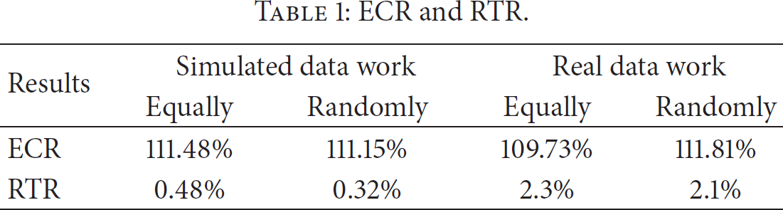
Energy Cost Ratio (ECR). ECR is defined as the energy cost proportion that the greedy algorithm compares with the Hungarian one, which is a key metrics to make comparison between the Hungarian algorithm and our greedy algorithm.

Running Time Ratio (RTR). RTR is defined as the running time proportion that the greedy algorithm compares with the Hungarian one during the process of finding optimal solution of data routing.

In every scenario, we would contrast our strategy to the condition that all the data are not allocated and wait the ships to pass through for collection. We call the strategy that data wait for collecting original strategy (OS) and our strategy DCEP.

5.1. Ship Trace Collection

In order to find the mobility pattern of ships, we put the devices (as Figure 5 shows) with general packet radio service (GPRS) modules DTP-S09 on ships. Each device is equipped with a SIM card. The GPS data is transmitted through the VPN of National Bureau of Oceanography provided by China Mobile Communications Corporation (CMCC) to our database every minute. Through two months (from 2011-07-01 to 2011-08-31) work, we collect the GPS data of 40 ships.

Figure 5

The GPS data collection devices.

5.2. Simulation

In first scenario, we set a 10 km $\times$ 10 km area and 3 fusion paths that their weight factors are, respectively, 3, 2, and 1. Ships crossing the area would select the path by their weight factors. That means it has the 50% probability of sailing along path 1, 33.3% along path 2, and 16.7% along path 3. To be closer to real life, the sailing paths would not be strictly the same with the fusion path. We add some random Gaussian distribution disturbances when the ship sails along one fusion path. We run our simulation in two different conditions, sensors equally deployed and sensors randomly deployed.

Figure 6(a) illustrates the result on data collection ratio of the condition that 169 sensors are equally deployed in the area. As more ships cross the area, the DCR is continuously increasing in DCEP. Comparing DCEP and OS, with increasing amount of ships passing through the area, the DCR of DCEP continues to rise until 94.80%. DCR of OS raises nearly the same with DCEP before the passing of 5 ships; however, the growth of the DCR starts to decline after the passing of 5 ships and DCR finally stops at 35.71%.

Figure 6

Data collection ratio of simulated data.

Figure 6(b) illustrates the result on data collection ratio of the condition that 220 sensors are randomly deployed in the area. All results present the same rule as the sensors are equally deployed. With increasing amount of ships passing through the area, the DCR of DCEP continues to rise until 97.91%. However, the growth of the DCR starts to decline after the passing of 5 ships and DCR finally stops at 36.33%.

5.3. Real Data Analysis

As we mentioned in Sections 1 and 2, we collect the GPS data of 40 ships in The Yellow Sea of China over two months. In the second scenario, we use the real data of ship traces to run our simulation. In the process of data analysis, we found that different ships used similar path while sailing from one certain location to a certain target. So, we choose a region from $124.0 6^{°}$ E to $124.1 2^{°}$ E and $39.66 5^{°}$ N to $39.7 1^{°}$ N to verify our strategy. As shown in Figure 8, we use the GPS data from 2011-08-01 to 2011-08-05 (color red) to generate two estimated paths (color blue). We use the traces in the next several days to simulate the procedure of data collection.

Figure 7(a) illustrates the result on data collection ratio of the condition that 49 sensors are equally deployed in the area. With increasing amount of ships passing through the area, the DCR of DCEP continues to rise until 100.00%. DCR of OS raises nearly the same with DCEP at the beginning. However, the growth of the DCR starts to decline after the passing of 4 ships and DCR finally stops at 79.92%.

Figure 7

Data collection ratio of real trace data.

Figure 8

Fusion path and traces from 2011-08-01 to 2011-08-05.

From Figure 7(a), we find that the OS collects more data than the DCEP at the beginning. Some sensors away from the fusion paths may store little or even no data after the allocation procedure. However, all the sensors have data at the beginning in OS. Because the ships are not strictly sticked to the fusion path during sailing, the DCEP may collect less data than OS at the beginning due to passing along sensors away from fusion paths, but after several ships passed, the DCR of DCEP would increase faster.

Figure 7(b) illustrates the result on data collection ratio of the condition that 50 sensors are randomly deployed in the area. With increasing amount of ships passing through the area, the DCR of DCEP continues to rise until 100%. However, the growth of OS DCR starts to decline after 4 ships passing and the DCR finally stops at 75.38%.

5.4. Algorithm Evaluation

During the process of simulation, we evaluate the performance of two algorithms during data routing process. From Table 1, we find that the energy cost of the greedy algorithm is nearly 11% more than that of the Hungarian one. However, the running time of the greedy algorithm is only a small part of the Hungarian one's. The data capacity of first scenario is 800–1100 MB, and data capacity of first scenario is 200–300 MB. As our result shows, the more data are stored in monitoring area, the more efficient the greedy algorithm will be without wasting more energy.

Table 1

ECR and RTR.

Results	Simulated data work		Real data work
Results	Equally	Randomly	Equally	Randomly
ECR	111.48%	111.15%	109.73%	111.81%
RTR	0.48%	0.32%	2.3%	2.1%

6. Related Work

In this section, we introduce some researches related to our paper. The research on underwater environment monitoring has drawn amount of attention, and some real-world systems have been deployed [1, 3, 5, 6]. Also some researchers have designed some strategy to monitor the ocean [4]. There are three kinds of data collection strategy in these systems. The first strategy of data collection is to deploy wired network to realize the data transmission. SNUSE is deployed for seismic monitoring and oil exploitation. The underwater network uses the wired sensors to realize collaboration of each sensor [3]. This kind of system could realize the effective and real-time data collection. However, building and maintaining a wired underwater network would use large costs. The second strategy is to collect data through satellites. Sea-web introduces a US Navy's underwater sensor network which can monitor the condition of underwater. The sensor reports its data to the buoy which could communicate with the base station by satellite or radio [1]. But satellite communication would not only increase the cost but also shorten the lifetime of the network. The third strategy is using data mules to realize environment monitoring or data collection. The AOSN and ASAP are monitoring schemas deploying autonomous underwater vehicles (AUVs) to monitor the area and predict the future conditions. They collect the data through glider network, base station, and the recovery of AUVs [2, 5]. This kind of strategy needs to deploy special equipments for long-term work. Our team did lots of researches on environment monitoring [27–29].

The mentioned researches are all designed for underwater environment monitoring. To achieve data collection, the systems always use satellites, data mules, and wired sensors, which significantly increase the cost. The delay tolerant network provides a by-product method to realize data collection or message delivery. In [30], Zhang et al. describe a delay tolerant network to monitor the behavior custom of wild animal called ZebraNet. DakNet wireless network takes advantages of the transportation which has communication modules to distribute the connectivity to developing villages [10]. Burgess et al. set an experiment which use buses to test his routing algorithm [18]. The above systems use the concept of delay tolerant network to collect or transmit the data by making use of the mobility pattern of animals and vehicles. For further study on mobility pattern of vehicles, Zhu and Ni present an innovative scheme to collect vehicles GPS data [31] and summarize the intercontact time and mobility pattern in urban VANETs [32]. He et al. provided some target tracking strategies with WSN [33, 34]. Li et al. designed an algorithm of sensor network navigation without locations [35]. However, the prior researches focus on the terrestrial network.

In this paper, we conduct an experiment to collect the GPS data of 40 ships to discover the mobility pattern of ships. Based on the mobility pattern of ship, we provided a data collection strategy which uses the ships of daily work to achieve data collection without the help of special data mules.

7. Conclusion

In this paper, we present a data collection strategy based on estimated path in ocean delay tolerant network. Through performance evaluation with both real data and simulated data, we prove that our method is effective. By this strategy, the data monitoring system could collect the data faster than ever without the help of special data mules. We also provide a feasible method to summarize the mobility pattern of ships which could be used to further study of the intrusion detections and location forecast.

Nevertheless, many issues still remain to be explored. Our ongoing works are $(1)$ finding out a plan that solves this problem under the circumstance that different ships have different speed and $(2)$ providing a strategy that could solve this problem under sparse sensor deployment.

Footnotes

Conflict of Interests

The authors declare that there is no conflict of interests regarding the publication of this paper.

Acknowledgment

This work was supported by the National Natural Science Foundation of China Grants 61170258, 61103196, 61379127, and 61379128.

References

Rice

Green

Underwater acoustic communications and networks for the US navy's seaweb program

Proceedings of the 2nd International Conference on Sensor Technologies and Applications (SENSORCOMM '08)

August 2008

Cap Esterel, France

715 722

10.1109/SENSORCOMM.2008.137

Vasilescu

Kotay

Rus

Dunbabin

Corke

Data collection, storage, and retrieval with an underwater sensor network

Proceedings of the 3rd International Conference on Embedded Networked Sensor Systems (SenSys '05)

2005

154 165

10.1145/1098918.1098936

SNUSE

http://www.isi.edu/ilense/snuse/

Yang

Liu

Sea depth measurement with restricted floating sensors

ACM Transactions on Embedded Computing Systems 2013 13 1, article 1

10.1145/2512448

Autonomous Ocean Sampling Networks II

http://www.princeton.edu/~dcsl/aosn/

ASAP

http://www.princeton.edu/~dcsl/asap/

Bokser

Oberg

Sukhatme

Requicha

A small submarine robot for experiments in underwater sensor networks

Proceedings of the International Federation of Automatic Control Symposium on Intelligent Autonomous Vehicles (IFAC '04)

2004

Dunbabin

Roberts

Usher

Winstanley

Corke

A hybrid AUV design for shallow water reef navigation

Proceedings of the IEEE International Conference on Robotics and Automation (ICRA '05)

April 2005

Barcelona, Spain

2105 2110

2-s2.0-33748907007

10.1109/ROBOT.2005.1570424

Zhao

Ammar

Zegura

A message ferrying approach for data delivery in sparse mobile Ad Hoc networks

Proceedings of the 5th ACM International Symposium on Mobile Ad Hoc Networking and Computing (MoBiHoc '04)

May 2004

187 198

2-s2.0-4444277059

10.

Pentland

Fletcher

Hasson

Daknet: rethinking connectivity in developing nations

Computer 2004 37 1 78 83

10.1109/MC.2004.1260729

11.

Jain

Shah

R. C.

Brunette

Borriello

Roy

Exploiting mobility for energy efficient data collection in wireless sensor networks

Mobile Networks and Applications 2006 11 3 327 339

2-s2.0-33646575292

10.1007/s11036-006-5186-9

12.

Kansal

Somasundara

A. A.

Jea

D. D.

Srivastava

M. B.

Estrin

Intelligent fluid infrastructure for embedded networks

Proceedings of the 2nd International Conference on Mobile Systems, Applications and Services (MobiSys '04) 2004 111 124

2-s2.0-4544231245

13.

Parker

Kansal

Somasundara

A. A.

Jea

D. D.

Strivastava

M. B.

Estrin

UCLA DTN Sensor Networks Update, 2004, http://www.dtnrg.org

14.

Zhang

Kurose

J. K.

Levine

B. N.

Towsley

Zhang

Study of a bus-based disruption-tolerant network: mobility modeling and impact on routing

Proceedings of the 13th Annual ACM International Conference on Mobile Computing and Networking (MobiCom '07)

September 2007

195 206

2-s2.0-37849041028

10.1145/1287853.1287876

15.

Heidemann

Wills

Syed

Research challenges and applications for underwater sensor networking

Proceedings of the IEEE Wireless Communications and Networking Conference (WCNC '06)

April 2006

228 235

2-s2.0-34250365027

16.

Caruso

Paparella

Vieira

L. F. M.

Erol

Gerla

The meandering current mobility model and its impact on underwater mobile sensor networks

Proceedings of the 27th IEEE Communications Society Conference on Computer Communications (INFOCOM '08)

April 2008

Phoenix, Ariz, USA

771 779

2-s2.0-51349086035

10.1109/INFOCOM.2007.53

17.

Akyildiz

I. F.

Pompili

Melodia

Underwater acoustic sensor networks: research challenges

Ad Hoc Networks 2005 3 3 257 279

2-s2.0-13944252629

10.1016/j.adhoc.2005.01.004

18.

Burgess

Gallagher

Jensen

Levine

B. N.

MaxProp: routing for vehicle-based disruption-tolerant networks

Proceedings of the 25th IEEE International Conference on Computer Communications (INFOCOM '06)

April 2006

Barcelona, Spain

1 11

2-s2.0-39049118503

10.1109/INFOCOM.2006.228

19.

Pompili

Melodia

Akyildiz

I. F.

Routing algorithms for delay-insensitive and delay-sensitive applications in underwater sensor networks

Proceedings of the 12th Annual International Conference on Mobile Computing and Networking (MobiCom '06)

September 2006

298 309

2-s2.0-33751062901

20.

Jain

Fall

Patra

Routing in a delay tolerant network

Proceedings of the Conference on Applications, Technologies, Architectures, and Protocols for Computer Communications (SIGCOMM '04)

September 2004

145 158

2-s2.0-21844451437

10.1145/1030194.1015484

21.

Chaintreau

Hui

Crowcroft

Diot

Gass

Scott

Impact of human mobility on opportunistic forwarding algorithms

IEEE Transactions on Mobile Computing 2007 6 6 606 620

2-s2.0-34247596905

10.1109/TMC.2007.1060

22.

Burns

Brock

Levine

B. N.

MV routing and capacity building in disruption tolerant networks

Proceedings of the IEEE INFOCOM 2005

March 2005

Miami, Fla, USA

398 408

2-s2.0-25844501977

23.

Heidemann

Estrin

An energy-efficient MAC protocol for wireless sensor networks

Proceedings of the IEEE 21st Annual Joint Conference of the IEEE Computer and Communications Societies (INFOCOM '02)

June 2002

1567 1576

2-s2.0-0036343658

10.1109/INFCOM.2002.1019408

24.

Liu

Iso-Map: energy-efficient contour mapping in wireless sensor networks

Proceedings of the 27th International Conference on Distributed Computing Systems (ICDCS '07)

June 2007

Toronto, Canada

2-s2.0-34848862157

10.1109/ICDCS.2007.115

25.

Dijkstra

E. W.

A note on two problems in connexion with graphs

Numerische Mathematik 1959 1 1 269 271

2-s2.0-34147120474

10.1007/BF01386390

26.

Kuhn

H. W.

The Hungarian method for the assignment problem

Naval Research Logistics 2005 52 1 7 21

2-s2.0-13144282754

10.1002/nav.20053

27.

Guo

Liu

Feng

Hong

CCSA: a cloud computing service architecture for Sensor Networks

Proceedings of the International Conference on Cloud and Service Computing (CSC '12)

November 2012

Shanghai, China

25 31

10.1109/CSC.2012.12

28.

Liu

Zhang

Guo

Component-based cloud computing service architecture for measurement system

Proceedings of the IEEE International Conference on Green Computing and Communications (GreenCom) and IEEE Cyber, Physical and Social Computing and Internet of Things (iThings/CPSCom '13)

August 2013

Beijing, China

1650 1655

10.1109/GreenCom-iThings-CPSCom.2013.299

29.

Guo

Liu

Wang

Jiang

Zheng

CVIS: complex virtual instruments system architecture

Proceedings of the IEEE International Instrumentation and Measurement Technology Conference (I2MTC '13)

May 2013

Minneapolis, Minn, USA

566 571

10.1109/I2MTC.2013.6555480

30.

Zhang

Sadler

C. M.

Lyon

S. A.

Martonosi

Hardware design experiences in ZebraNet

Proceedings of the 2nd International Conference on Embedded Networked Sensor Systems (SenSys '04)

November 2004

ACM

227 238

2-s2.0-27644529341

31.

Zhu

L. M.

HERO: online real-time vehicle tracking in Shanghai

Proceedings of the IEEE 27th Conference on Computer Communications (INFOCOM '08)

April 2008

Phoenix, Ariz, USA

942 950

10.1109/INFOCOM.2008.147

32.

Zhu

Xue

Zhu

L. M.

Recognizing exponential inter-contact time in VANETs

Proceedings of the IEEE INFOCOM 2010

March 2010

San Diego, Calif, USA

1 5

2-s2.0-77953309373

10.1109/INFCOM.2010.5462263

33.

Vicaire

Yant

Luo

Zhou

Stoleru

Cao

Stankovic

J. A.

Abdelzaher

Achieving real-time target tracking using wireless sensor networks

Proceedings of the 12th IEEE Real-Time and Embedded Technology and Applications Symposium

April 2006

37 48

2-s2.0-33749595383

10.1109/RTAS.2006.9

34.

Huang

Blum

B. M.

Stankovic

J. A.

Abdelzaher

T. F.

Range-free localization and its impact on large scale sensor networks

ACM Transactions on Embedded Computing Systems 2005 4 4 877 906

10.1145/1113830.1113837

35.

Liu

Wang

Yang

Sensor network navigation without locations

Proceedings of the IEEE INFOCOM 2009

April 2009

Rio de Janeiro, Brazil

2419 2427

2-s2.0-70349686611

10.1109/INFCOM.2009.5062169

DCEP: Data Collection Strategy with the Estimated Paths in Ocean Delay Tolerant Network

Abstract

1. Introduction

2. Estimated Path Generation

2.1. Trace Analysis

2.2. Distance between Two Curves

2.3. Path Fusion

Algorithm 1: Path fusion.

3. Data Allocation Strategy

3.1. Transmission Capacity of Path

3.2. Data Allocation Strategy in Path Level

3.3. Data Allocation Strategy in Node Level

4. Data Routing

4.1. The Process of Data Routing

4.2. The Optimal Routing Plan

4.3. The Greedy Algorithm

Algorithm 2: Greedy algorithm.

5. Performance Evaluation

5.1. Ship Trace Collection

5.2. Simulation

5.3. Real Data Analysis

5.4. Algorithm Evaluation

6. Related Work

7. Conclusion

Footnotes

Conflict of Interests

Acknowledgment

References