Sage Journals: Discover world-class research

Abstract

A single-sided induction heating system based on IGBT is proposed. The system includes the series resonant circuit, control circuit, and auxiliary circuit. The main circuit includes rectifier, filter, inverter, and resonant circuit. A drive circuit is designed for IGBT combing some protection circuits. We have a simulation of the single-sided induction heating system in ANSYS. The simulation results are compared with the experimental results. The performance of the system is promising. And also we estimate the temperature distribution model by the least squares theory.

1. Introduction

The electromagnetic induction heating technology, which is known as the “green heat” mode, is increasingly being used in areas of industrial production and civil applications, such as industrial electronic encapsulation, surface quenching, melting technology, civil induction cooker, and water heater, due to its high efficiency, security, and other significant advantages [1]. Induction heating power is a kind of inverter device which converts alternating current power to the middle frequency alternating current, high frequency, or ultrasonic frequency alternating current by electromagnetic induction principle to change electrical energy into heat energy [2]. It has the characteristics of easily achieving automatic control, the short heating time, and high temperature [3]. The high temperature is particularly important for precious metals. Induction heating efficiency is higher than the flame furnace with about 30%∼50% and higher than traditional electric resistance furnace with about 20%∼30% and it has the advantages of convenient operation and long service life [4]. This paper introduced the design of IGBT induction heating equipment which was used on the single surface. Firstly we introduce the principle of single induction heating. Second we introduce the selection and design of main circuit and other parts of system. Then we do some simulations and experiments and have a conclusion finally.

2. The Principle of Single Induction Heating

Single induction heating is based on the principle of electromagnetic induction [2]. Due to the impedance of conductive substance, the power on the impedance is converted into heat energy. So it achieves the heating of the workpiece, as shown in Figures 1 and 2.

Figure 1:

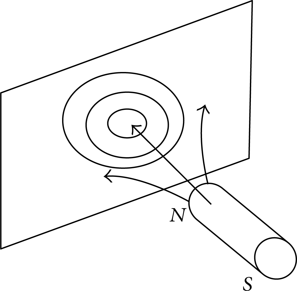
The principle of single-sided heating.

Figure 2:

Induction heating effect.

According to Maxwell's electromagnetic equation the induction electromotive force is as follows when the alternating magnetic Φ = Φ_msinωt:

e = - N \frac{d Φ}{d t} = - N Φ_{m} ω \cos ω t,

(1)

where N is the coil number of turns, Φ is the flux, and e is the inductive electromotive force.

And then we can calculate the effective value of eddy current in the cross section

I_{2} = \frac{E}{Z} = \frac{E}{\sqrt{R^{2} + X_{L}^{2}}},

(2)

where R is the equivalent resistance of the heated metal workpiece and $X_{L}^{}$ is the equivalent impedance of eddy current circuit.

The role of induction coil is electricity transmission, which transfers the electrical energy into heat energy within the metal artifacts [5]. Its power can be expressed as

P = 0.24 I_{2}^{2} R = \frac{4.73 N^{2} f^{2} Φ_{m}^{2} R}{R^{2} + X_{L}^{2}} .

(3)

When the load is fixed, the heating power depends on the magnetic field intensity and frequency. So you can increase the current amplitude in the coil and frequency to enhance the heating effect. In addition, the cross-sectional shape of the metal, section size, permeability, and conductivity can also influence induced eddy current [4, 6 –8].

Due to the influence of the skin effect, the conductor induce eddy in the alternating magnetic field eddy current along the conductor surface to another surface is attenuation accordance with the law of index. The depth δ is called the current penetration depth when the vortex intensity attenuation reaches the 1/e (36.8%) of its maximum value. Penetration depth can be determined by the following expression:

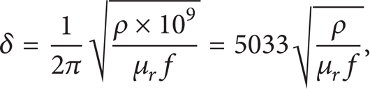
δ = \frac{1}{2 π} \sqrt{\frac{ρ \times 1 0^{9}}{μ_{r} f}} = 5033 \sqrt{\frac{ρ}{μ_{r} f}},

(4)

where δ is the current penetration depth, the ρ stands for artifacts, f is relative permeability of workpiece, and f is the current frequency.

We can see from formula (4), when the material properties are given, penetration depth is only related to frequency. So we can adjust the frequency to control the heating of the workpiece thickness.

3. Design of a Half-Bridge Series Resonance Circuit

Heating coil and the workpiece form a load of induction heating power. It can be equivalent to inductance and small resistance in series (L,R in Figure 3(a). As phase difference of the current and voltage is close to 90°, the power factor is extremely low. The capacitor is always used to compensate reactive power to improve the power factor. According to the connection of capacitor C and coil, it can form two basic types of inverter: series resonant voltage type inverter and parallel resonant inverter (current mode) [9]. The inverter power supply is different for different types of inverter. Large capacitor is often used in voltage type inverter to provide stable dc voltage. And reactor is often used in the current type inverter to provide a smooth dc current. The full-bridge inverter circuit, respectively, is shown in Figures 3(a) and 3(b) [10].

Figure 3:

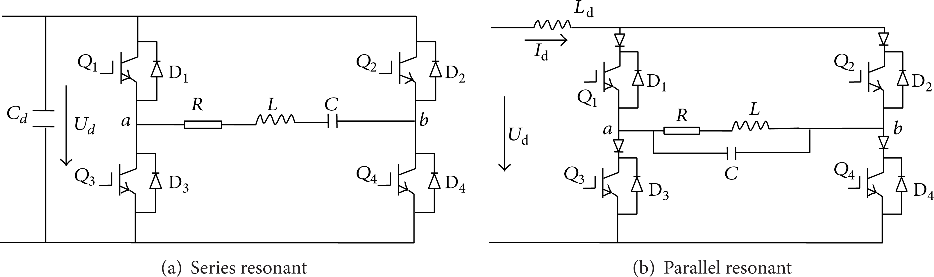
Series and parallel inverter circuit.

The Analysis of the Series Resonance Circuit. In Figure 3(a), supposing the voltage on LCR is $\overset{\cdot}{U} = U_{m} \sin w t$ , the current of LCR will be

\overset{\cdot}{I} = \frac{\overset{\cdot}{U}}{\overset{\cdot}{Z}} = \frac{\overset{\cdot}{U}}{R + j (w L - (1 / w C))} .

(5)

When the impedance is equal to the capacitive reactance, namely, X_L = X_C, $w L = (1 / w C)$ , the current of the series circuit is the maximum. It is the resonant state. At this point, X = 0, the impedance $\overset{\cdot}{Z} = R$ , and angular frequency $w = (1 / \sqrt{L C})$ equals the inherent resonant angular frequency of the circuit $w_{0} = (1 / \sqrt{L C})$ .

In the resonance, the voltage of the capacitance and the inductor are, respectively,

\begin{matrix} {\overset{\cdot}{E}}_{C 0} = \frac{1}{j w_{0} C} \frac{\overset{\cdot}{U}}{R} = - j \frac{\overset{\cdot}{U}}{w_{0} C R} = - j Q \overset{\cdot}{U}, \\ {\overset{\cdot}{E}}_{L 0} = j w_{0} L \frac{\overset{\cdot}{U}}{R} = j Q \overset{\cdot}{U} = - \overset{\cdot}{E_{C 0}} . \end{matrix}

(6)

$Q = (w_{0} L / R) = (1 / w_{0} C R) = (1 / R) \sqrt{L / C}$ is the quality factor of resonance circuit. When the resonance occurs, the voltage of the resistance is the supply voltage. The voltage of inductance and capacitance is converse, so it is called voltage resonant.

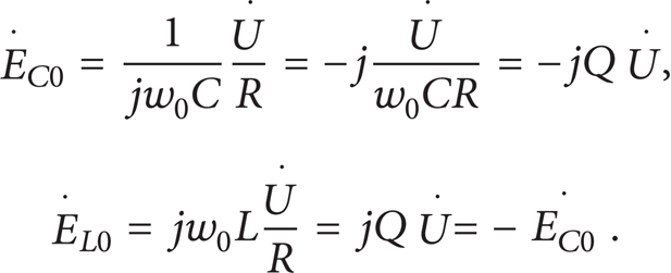
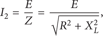
The effective value of the current is

I = \frac{U}{Z} = \frac{U}{R \sqrt{1 + Q^{2} {((w / w_{0}) - (w_{0} / w))}^{2}}} = \frac{I_{0}}{\sqrt{1 + Q^{2} {((w / w_{0}) - (w_{0} / w))}^{2}}},

(7)

where $I_{0} = (U / R)$ is the effective value of the current when the resonance occurs; for convenience of study, it is written by

\frac{I}{I_{0}} = f (\frac{w}{w_{0}}) .

(8)

We can draw Figure 4 when $(w / w_{0})$ is x-axis and $(I / I_{0})$ is y-axis. The curves show that the larger the Q, is the more severely the resonant curve changes. That is why it is called the quality factor. In the diagram, left of the $(w / w_{0}) = 1$ line stands for the capacitive area (capacitive reactance is greater than the impedance) and right side is the perceptual area (inductive reactance is greater than the capacitive reactance). In the series resonance, the system generally works in weak emotional state in order to improve the security performance of the inverter circuit.

Figure 4:

The resonant diagram under different Q.

4. The Design of the Induction Heating System

4.1. The Topology of the System

The system topology is shown in Figure 5; the main function of the main circuit is to achieve power conversion, including the power input grid harmonic filter, three-phase rectifier unit, filtering unit after rectifying, the half-bridge inverter unit used to produce high frequency alternating current (ac), the transformer used for load matching, load unit composed of heating coil, and the workpiece. The main function of the auxiliary circuit is to provide necessary service functions for normal operation of the main circuit, such as power supply, voltage, current and temperature detection and protection circuit, drive circuit of the inverter unit, and the control of the signal processing circuit.

Figure 5:

The topology of the system.

4.2. The Selection of Operating Frequency and Power

In a single induction heating system, the power and frequency of current are the most critical parameters of induction heating power, which play a leading role in the thermal efficiency of heating system, the efficiency of electricity, and the quality of heated workpiece.

In the frequency selection of single induction heating device, we should consider the electricity efficiency, thermal efficiency, the temperature difference between the surface and internal requirement and the heating depth, and other factors comprehensively. For the single heating of steel, in order to obtain higher thermal efficiency, achieve good energy saving effect, and shorten the heating time, the current penetration depth general should be set to be 1–3 times the depth of heating according to engineering experience. At this time, the current frequency can be expressed as

f = \frac{(2.8 ~ 25.3) \times 1 0^{8} ρ}{μ_{r} D_{S}^{2}} (Hz),

(9)

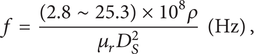
where D_S is the heated depth and the unit is mm; ρ is the material resistivity Ω·cm; μ_r is the relative permeability.

The heat capacity of the heated material, the size of the workpiece, and the frequency of the applied current are the main factors in single-sided heating power, and the production efficiency is generally considered in industrial production. The induction heating power can be expressed as

P_{i} = P_{R P} + P_{L 2} + P_{L 1},

(10)

where the power of the total input is on the left of equal sign; the right-hand side in the first one is the effective power for heating the workpiece, the second one is the loss due to the heat conduction, convection, and radiation, and the third one is the wastage of the inverter, such as the loss of switching, conduction losses, and heat loss of induction coil. Due to the fact that the influence factors are more, the power should be expressed as follows in the design of induction heating power in engineering:

P_{i} \approx (1.5 ~ 1.6) P_{R P} .

(11)

For single-sided heating of steel, the effective power can be express as

P_{R P} = \frac{C_{W} \cdot a \cdot S \cdot h \cdot Δ T}{t} .

(12)

The heating area of workpiece is S (m²), the heating depth is h (m), the heat capacity C_W (kW·h/(kg·°C)) of the workpiece can be thought to be fixed, the material density is a (kg/m after), the heating time is t (s), and the temperature is ΔT (°C).

4.3. IGBT Drive

IGBT is a three-terminal device, and it has the advantages of the voltage drive, low bipolar transistor turn-on voltage, and small output impedance [11], which determine the driving conditions of IGBT. The performance of the IGBT gate driving circuit has a direct effect on the system constructed by the IGBT. Drive circuit generally should have the function of reliable drive, over voltage, over current, and du/dt protection.

According to the above requirements, output power, maximum output current, the highest working frequency, signal isolation, grid resistance, and other factors should be considered when designing the IGBT driver driving circuit. In the single electromagnetic induction heating system, the load is general weak perceptual, and interference is big. In order to ensure reliable open and shut off IGBT under large disturbance, we provide a ± 15 v voltage for grid emitter of IGBT. If the grid-emitter voltage of IGBT exceeds the limit (usually of ± 20 v), the IGBT will be permanent damage, so there is an amplitude limiting circuit for the grid voltage.

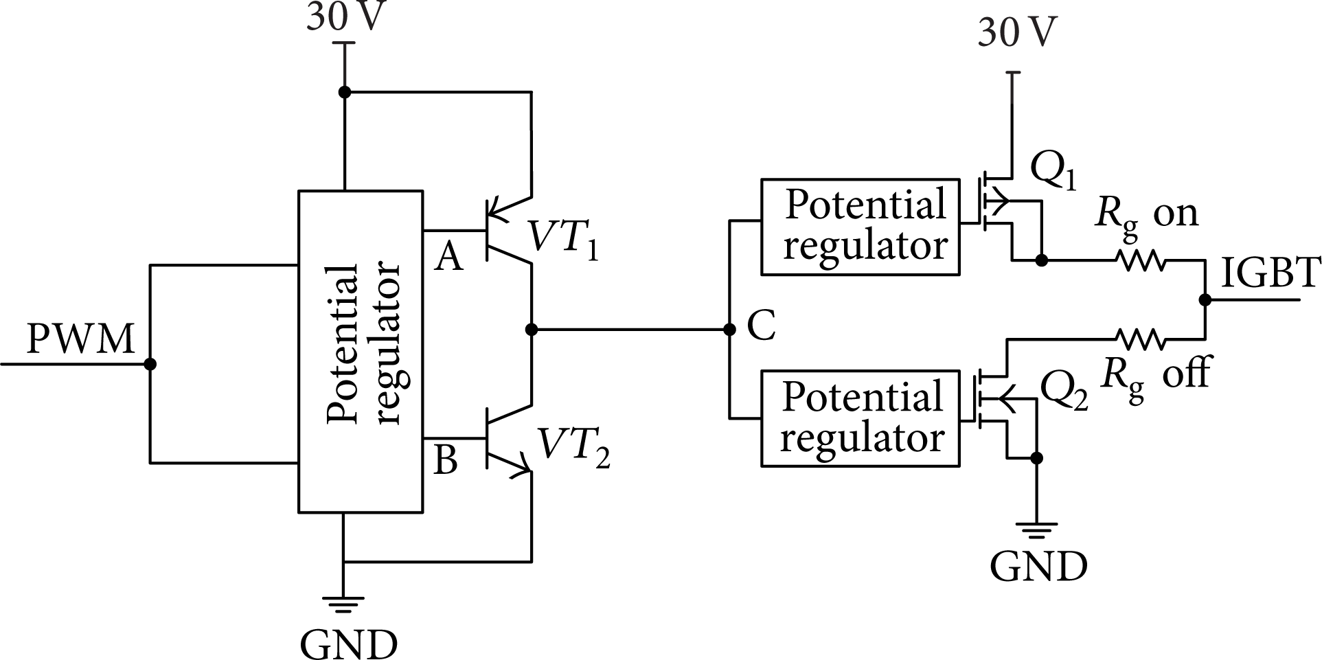
In order to provide the ± 15 v voltage for grid emitter, two kinds of power supply scheme have been designed; the first one is the single 30 v power supply (the emitter voltage is 15 v and the grid voltage is 0–30 v) and the other one is the ± 15 v power supply (the power of the upper tube is 15 v and the power of lower tube is −15 v), and finally does push-pull output. The voltage of grid emitter will be ± 15 v when the upper and lower IGBT turn on alternately. In the two driving circuits, the optical coupling isolation, IGBT retreat saturation detection, protection, and fault signal output function are included. The output stage design is shown in Figures 6 and 7, respectively.

Figure 6:

Single 30 v power drive circuit.

Figure 7:

± 15 v power drive circuit.

The use of ± 15 V, such as Figure 7, there is no other device requirements due to the fact that the devices can work at 15 V. The circuit topology uses MOSFET driver chip, MOSFET, and bipolar transistor forms the bipolar transistor output stage which is push-pull output; the output impedance is relatively small, which is required by the driving circuit, and both have two transistors up and down. Therefore, the current output is greater. Also the potential role of conditioning circuit is to provide a suitable MOSFET gate voltage. The driving waveform is shown in Figure 8.

Figure 8:

± 15 v power drive circuit physical and driving waveform.

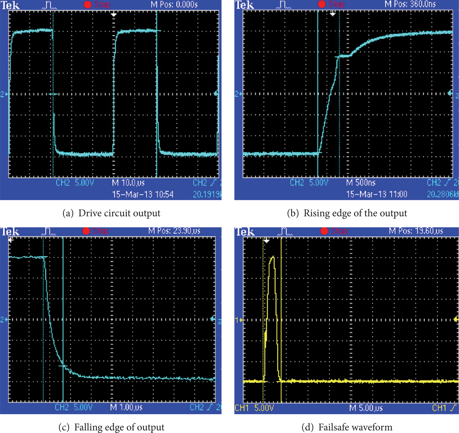
Using a single 30 v power as shown in Figure 9, it can be seen from the figure that the output of the drive circuit is relatively smooth on both rising and falling edges. The figure can clearly reflect the Miller platform. When a fault occurs, IGBT can withstand short-circuit time that is about 10 μs; the fault protection in Figure 8 can be seen when short fault occurs, IGBT conduction time can be left in 3 μs, which can effectively protect the IGBT. In the system of this paper, the single 30 v power is used.

Figure 9:

Single 30 v power drive circuit physical and driving waveform.

4.4. The Resonant Circuit Design

Compared with the general induction heating, the resonant circuit of single induction heating design is a difficult work to achieve during the system design [12]. The resonant circuit includes a resonant inductor, a compensation capacitor, a load matching transformer, a heating coil, and the workpiece. The circuit is shown in Figure 10.

Figure 10:

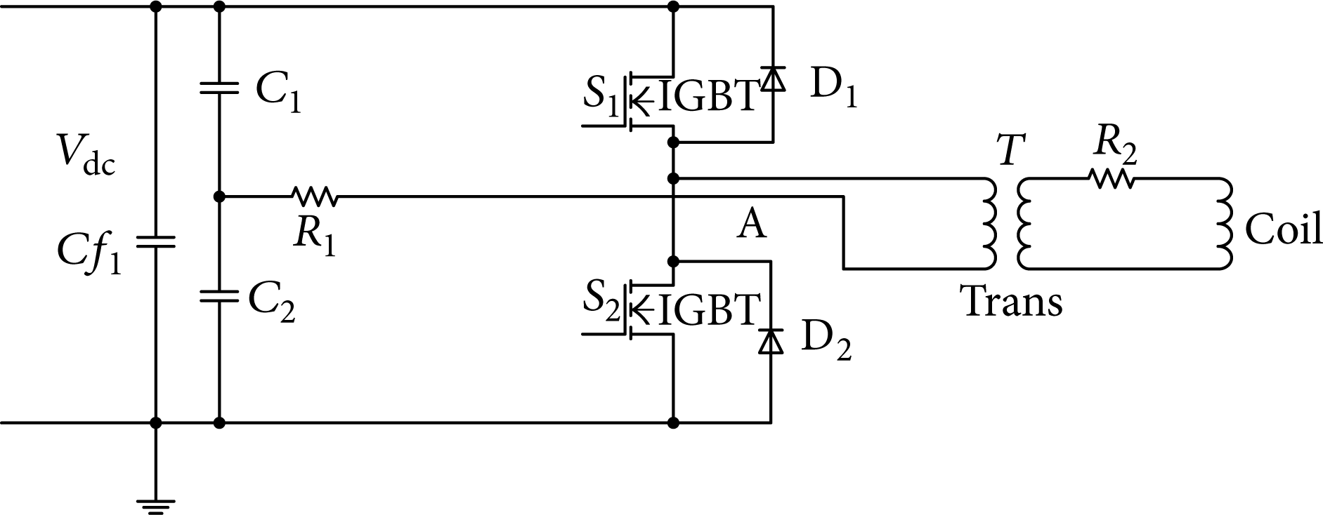
The resonant circuit.

4.4.1. Induction Coil Design

In the high-frequency heating applications, the heating coils are the first things to consider; we need to choose the right material and winding shape [13]. The coils should be based on the current flowing through the coil to be determined. In our prototype of single induction heating, we use a planar spiral coil, and the heating coil is shown in Figure 11 outline.

Figure 11:

Heating coil.

The inductance of the planar coil can be estimated by following formula:

L = K_{P} D N^{2} \times 10^{- 3},

(13)

where $K_{P} = 1000 D / (40.6 D + 111.7 δ)$ and the unit of L is μH. D is the average diameter of the reel; the unit is cm. N is the coil turns and δ represents the thickness of the coil; the unit is cm.

4.4.2. Matching Transformer Design

In order to make the load impedance be equal to the heating power of the nominal impedance, the load matching is required to be implemented. Electromagnetic coupling method [14] is commonly used in the series inverter power source by the high-frequency transformer. In the system, the primary is 16 turns, using high temperature 16 mm² wire GN-500 that is compose of thin wires, which leads internally by a plurality of thin wires connected in parallel, and the temperature can reach 500°C. The secondary side of the cylindrical coil is copper, so that all the primary sides can be surrounded, while increasing the carrying capacity of the secondary side. The transformer uses EE210 ferrite core, which allows for a power of 13 kW and is more suitable for the working conditions of more than 20 kHz. The transformer and heating coil are shown in Figures 12(a) and 12(b).

Figure 12:

Transformer and heating coils.

4.4.3. Determine the Value of Resonant Inductance of the Inductor

We can make use of the resonant voltage and current of the inductor to calculate the theoretical value of half-bridge series resonant inductor and the compensation capacitor and then calculate the capacitor values according to resonance condition [15]. When the resonance occurs, the voltage of the inductor and capacitor are Q times of inverter output voltage:

U_{L} = U_{C} = Q U_{H} = Q \frac{\sqrt{2}}{π} U_{d},

(14)

where U_H is the inverter output; with regard to the half-bridge series circuit, its value is $\sqrt{2} / π$ times of the DC bus voltage; the quality factor Q generally takes about 3. The desired value of the resonant inductor is

L = \frac{U_{L}}{ω I_{H}} = \frac{U_{L}}{2 π f I_{H}} .

(15)

After obtaining the inductance value, we can calculate the compensation capacitance value according to the inductive reactance which is equal to capacitive reactance. Namely,

ω L = \frac{1}{ω C} .

(16)

Then

C = \frac{1}{ω^{2} L} = \frac{1}{4 π^{2} f^{2} L} .

(17)

4.5. Safeguard

4.5.1. The Buffer Circuit Design of IGBT

During the work of IGBT, the voltage and current of both sides change very fast, with the presence of stray inductance; there will be switching voltage spikes, as shown in Figures 13(a) and 13(b).

Figure 13:

The voltage output and after adding buffer circuit (× 10).

The primary circuit parasitic inductance is the reason of voltage spikes. The snubber circuit is to suppress spikes and is an effective way to protect the IGBT. In the system, the buffer circuit is shown in Figure 14, which comes from C discharge suppressing; no sense capacitor C_s is to absorb the surge voltage of the IGBT, and the R_s can inhibit oscillation C_s and limit the current through the IGBT discharges.

Figure 14:

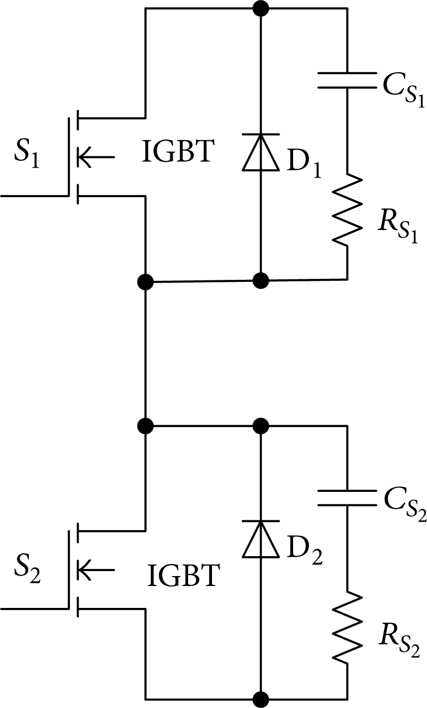
The buffer circuit.

The value of C_s can be estimated according to the principle of conservation of energy. In the estimation of C_s, the general standard is to absorb the energy stored in the stray inductance C_s. The voltage of capacitor cannot exceed the limit voltage of IGBT, namely,

\frac{1}{2} L_{s} I_{C}^{2} \leq \frac{1}{2} C_{S} U_{C E \max}^{2},

(18)

where L_s is the stray inductance of a circuit, I_C represents the current flowing through the IGBT, and U_CEmax is the withstand voltage limit of IGBT. According to formula (18) it can be obtained that

C_{S} \geq L_{s} \frac{I_{C}^{2}}{U_{C E \max}^{2}} .

(19)

According to the principle of suppressing oscillations, the value of resistor is

R_{S} > 2 \sqrt{\frac{L_{s}}{C_{S}}} .

(20)

4.5.2. Current Detection and Protection Circuit

In the process of heating operation, we need to sample the DC bus current in order to achieve real-time monitoring. In addition, the interference is complex under the high-frequency switching mode of operation of the induction heating power; these are likely to cause the overcurrent or short circuit. Therefore, the current signal is also essential; particularly, we need to control the heating power and frequency.

The Hall current sensor is used to collect current signals. In this system we use CSM100LA current sensor to collect the DC bus current. Current sampling and signal conditioning circuit are shown in Figure 15. RIN1 in the diagram is measuring resistor; U6 is a voltage reference chip, and it can output high-precision voltage.

Figure 15:

Current detection circuit.

The Hall sensor outputs current signal by measuring the voltage of resistance RIN1, after the op amp voltage follower and recuperate, it is sent to the AD port of microcontroller. After the microcontroller reads the signal, we can speculate the load conditions, and it can realize protective action when overcurrent occurs in the system.

4.5.3. Temperature Detection and Protection Circuit

The sustain current of the IGBT will decrease with temperature increasing; otherwise it causes permanent damage. Therefore, we need to have a protection circuit to stop the system when IGBT junction temperature rises to a certain extent. We usually use cooling device for cooling or real-time monitoring module to monitor the temperature. Figure 16 shows the temperature detection circuit. We use positive temperature coefficient thermistor as a temperature sensor. If the temperature exceeds a certain limit, the microcontroller will send the corresponding command according to the internal calculation.

Figure 16:

Module temperature sensing circuit.

In addition to the temperature monitoring of the IGBT module, we should use a cooling fan, so that the normal working of the device temperature can be maintained at a reasonable range.

5. Simulation Results

5.1. Main Circuit Simulation

According to the main circuit topology, we built simulation model in the MATLAB that is shown in Figure 17. It is used to control the half-bridge inverter pulses by the two-pulse signal generator. In the simulation model, the values of inductance, capacitance, and resistance in the inverter circuit can be determined according to actual measurements and calculation.

Figure 17:

Simulation model of the primary circuit.

Figure 18 shows the simulation for a given inductance 120 μH, resonant capacitor 0.5 μF, equivalent resistance 13.7 ohm, and the switching frequency 22 kHz. Figure 18(a) represents the inductor current and it is approximately sinusoidal; Figure 18(b) shows the voltage of the inductance and resistor due to the nonseparable resistance of the inductor coil. Therefore, the voltage of the resistance and inductor is between the square and sine. Figure 19 shows the voltage and current wave in practice, and we can see that the actual results and simulation results are very consistent.

Figure 18:

The current and voltage of inductor in simulation.

Figure 19:

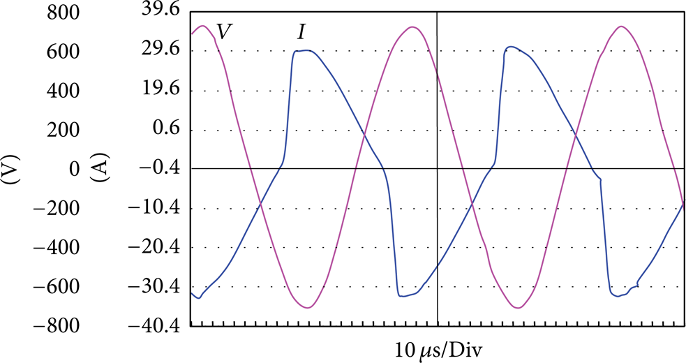
Actual current and voltage of inductor.

From the actual test, the voltage waveform across the inductor is different with different frequencies. If the system works in the inductive area, the closer the resonance point is, the closer the sinusoidal voltage wave will be, which is shown in Figure 20. It is close to a square wave when the point is far away from the resonance point. Considering it under the limiting case, up to a certain frequency, the capacitive reactance can be ignored compared with the inductive reactance, so the voltage across the inverter is almost added to the ends of the inductor.

Figure 20:

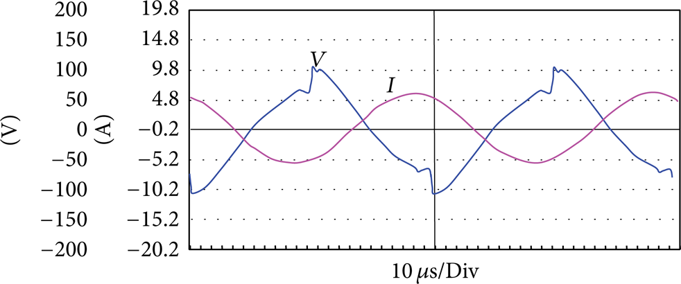
Current and voltage of inductor at resonant state.

The voltage wave in Figure 20 appears distorted in peak and trough, which is due to the commutation devices (switch and antiparallel diode), and the distortion position is related to the switching frequency. We can also see from the figure that the commutation time of the switch and antiparallel diode is the maximum current in the circuit, which is consistent to the previous half-bridge series resonant operation of the circuit analysis.

The voltage wave of C-E in half bridge at resonance state is shown in Figure 21; voltage distortion has occurred in rising and falling edges of the voltage wave. It corresponds to the voltage distortion in Figure 20, and the maximum value of the current also happens in this moment. If the circuit does not work in the resonant state, but in weak inductive state, the operating frequency is higher than the resonant frequency of the circuit; the corresponding wave is shown in Figure 22. The high and low stage has a significant level in the voltage wave, which is the commutation point of the nonresonant state.

Figure 21:

Output voltage and inductor current at resonant state.

Figure 22:

Output voltage and inductor current at nonresonant state.

The voltage wave of the capacitor measured in practice is shown in Figure 23, which is nonsymmetrical sinusoidal wave; it is caused by the process of charging and discharging of the capacitor.

Figure 23:

Voltage wave of the compensation capacitor.

5.2. The Temperature and Electromagnetic Field Simulation in ANSYS

For studying the internal mechanism of sided induction heating in depth, we make use of ANSYS to simulate the coupled relationship between electromagnetic field and temperature field [16, 17]. In the experiments, the workpiece dimension is 460 mm × 300 mm × 30 mm, 45 gauge steel; the heated workpiece is in axisymmetric shape, and then the electromagnetic field, eddy current field, and temperature field are also axisymmetric distributed. To reduce the amount of calculation, we take the 1/4 workpiece as the processing target. The three-dimensional model of the induction heating is shown in Figure 24. The large area outside is the surrounding air, which shows the coil and the workpiece (the bottom part), respectively. Regarding the geometric center of the lower surface of the workpiece as the origin of coordinates, along the longitudinal direction of the workpiece for the x-axis coordinate, width of the workpiece for the y-axis direction and the thickness direction of the workpiece for the z-axis coordinate direction are shown in the figure, respectively. There are three points located in the workpiece, A(75, 75, 30), B(75, 75, 15), and C(75, 75, 0); the three points are on the upper surface, the intermediate layer, and a lower surface of the workpiece.

Figure 24:

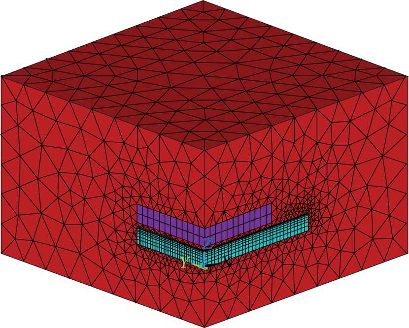
Three-dimensional and meshing models of single-sided heating.

The heated workpiece and the shape of the coil are fixed. The current frequency, eddy current density, and time are the major factors affecting the temperature distribution. Thus, the kinds of working conditions are tested to explore single-sided heating patterns and the above factors on the temperature distribution.

5.2.1. The System Analysis under Given Conditions

We do the simulations under the condition of current frequency f = 15 kHz; the current density is 5 * 10⁶ A/m; the air gap between the coil and the workpiece is 6 mm and the temperature is 20°C. Figure 25(a) shows the magnetic flux density vector across the surface of the workpiece, and Figures 25(a) and 25(b) show that the surface temperature distribution is not uniform. The maximum flux density, the highest temperature, and the highest eddy current density are not in the geometric center of the workpiece and the coil but in a peripheral zone from the center.

Figure 25:

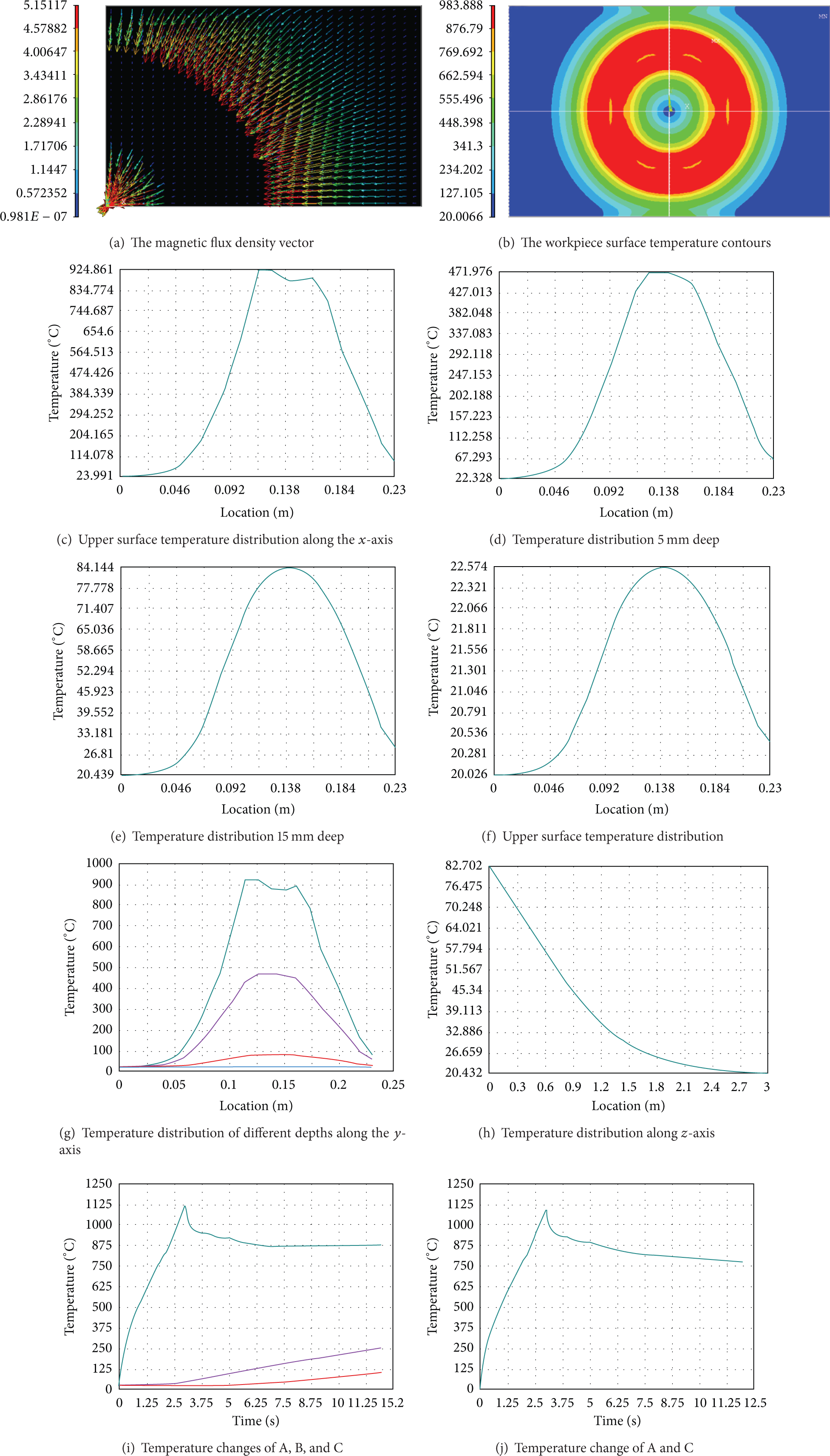
The comprehensive simulation results under given conditions.

Figures 25(c)–25(f) show the temperature distribution for 4's heating; the distance is 0, on the upper surface (the upper surface of the workpiece), 5, 15, and 30 mm (the lower surface of the workpiece) depth layer along the x-axis direction, respectively. These curves in the Figures can better match with Figures 25(a) and 25(b); the highest temperature point appears in the surrounding where in a certain distance from the geometric center of the workpiece. Figures 25(c)–25(f) show that maximum temperature of these deep layers is 924°C, 472°C, 84°C, and 23°C, which means that the surface temperature is almost constant. These figures also confirm the skin effect. The heat of the workpiece is mainly on the upper surface and descending along the plate thickness direction.

In order to better display the image of the temperature distribution along the direction of the plate thickness, the temperature distribution curves of different numbers of depth levels along the y-axis are put in the same graph, as shown in Figure 25(g). The distance from top to bottom on the upper surface is 0, 5, 15, and 30 mm (the lower surface of the workpiece) depth layer, respectively. It can be seen that the farther from the surface it is, the lower the temperature rises. Figure 25(h) shows the temperature gradient in the workpiece along the z-axis (the plate thickness direction); it can better show the concentrated heat caused by the skin effect of current.

Figures 25(i) and 25(j) show several key points’ temperature changes with time and the temperature difference between them. Figure 25(i) shows that the temperature of B and C points which are in the intermediate layer and the lower surface plate, respectively, changes very slow, whereas the temperature of point A in the upper surface rises very fast, almost linear up to the maximum value directly, declines when reached maximum temperature, and then leveled off. This is because the temperature of the workpiece over the Curie point and the surface of the heat are lost through three main ways: the cladding material absorbing energy to complete the phase change, heat transfer between the surface and the inner, and radiation to the surrounding air. Since this workpiece surface has lost magnetic, so the induced of the surface eddy currents is small; the heat generated by the Joule effect is less than the loss of energy, causing the temperature drop of the workpiece surface. The temperature difference between two corresponding values of A point and C point which located at the upper and lower surfaces is shown in Figure 25(j).

5.2.2. The Temperature Distribution under Different Frequencies

To explore the effect of different frequencies on single-sided induction heating process, eddy current density is maintained at 5 * 10⁶ A/min during the simulation and the frequency is set to different values to obtain the temperature along with the change of time at the A and C points, as shown in Figure 26. The curves are corresponding to 100 kHz, 50 kHz, 30 kHz, 20 kHz, and 15 kHz. The higher the frequency is, the higher amplitude temperature and change rates of the upper and lower surface will be. In Figure 26, the temperature variation of C point is extremely slow. Therefore, the temperature difference between A and C points is similar to point A. It can be concluded that the higher the frequency is, the larger the surface power density will be, and the surface temperature of workpiece will be faster rise and the greater, and the maximal temperature will be bigger when other conditions keep constant.

Figure 26:

The temperature difference of A and C under different frequencies.

Figure 27 shows the attenuation of workpiece temperature under different frequencies along the z-axis direction; the x-axis is the distance to the upper surface; the y-axis is the temperature along the axis; the heating time is 4's, and the curves are corresponding to the frequencies of 100 kHz, 50 kHz, 30 kHz, 25 kHz, 20 kHz, and 15 kHz from top to bottom. It can be clearly seen that, in the case of certain other conditions, the higher the frequency is, the higher temperature change rate along the direction of thickness of the workpiece will be. When the operating frequency is low, the induced eddy currents and the energy obtained by workpiece will be small. The temperature gradient of the plate thickness direction becomes small due to the heat conduction in a certain heating time.

Figure 27:

The temperature decay curve along the z-axis under different frequencies.

5.2.3. The Effect of Eddy Current Density on the Temperature Distribution

In the simulation, we change the eddy current density to analyze the relationship between temperature distribution and eddy current density. The temperature difference between points A and C is shown in Figure 28; the curves are corresponding to the eddy current density of 10*10⁶ A/m², 8*10⁶ A/m², 5*10⁶ A/m², 2*10⁶ A/m², and 1*10⁶ A/m² from left to right. From the figure we can know that the greater the eddy current density is, the greater the surface power density of the workpiece will be, and the faster the surface temperature of the workpiece rises, the higher the maximum temperature will be, which is similar to the influence of frequency. If the eddy current density is not too large (corresponding to the eddy current density of 2*10⁶ A/m² and 1*10⁶ A/m²), the surface temperature changes more relaxed; heat can be transmitted promptly to the internal and external parts, and the phenomenon of local overheating will not appear, but the heating time will be longer. When increasing the eddy current density or frequency to speed up the heating, the phase transition temperature on the surface will rise and the surface temperature of the flat areas will appear at a higher temperature region. It is easy to overheat.

Figure 28:

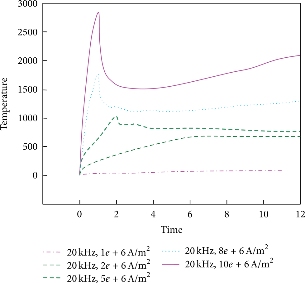
The temperature of A and C points under different vortex densities.

Figure 29 visually shows the attenuation of workpiece temperature under different frequencies along the z-axis; the x-axis is the distance to the upper surface; the y-axis is the temperature along the axis, and the heating time is 4's. Its analysis is similar to the relationship between temperature gradient and frequency of Figure 27.

Figure 29:

The temperature decay curve along the z-axis direction under different vortex densities.

Through the above analysis, in order to achieve the ideal temperature difference between upper and lower surfaces, we should reasonably control the heating frequency, eddy current density, and the heating time in single-sided heating. We can adjust heating depth by changing the time and eddy current density when a frequency is certain. If a thin heating thickness is required, the heating should be chosen larger surface power density, namely, higher operating frequencies.

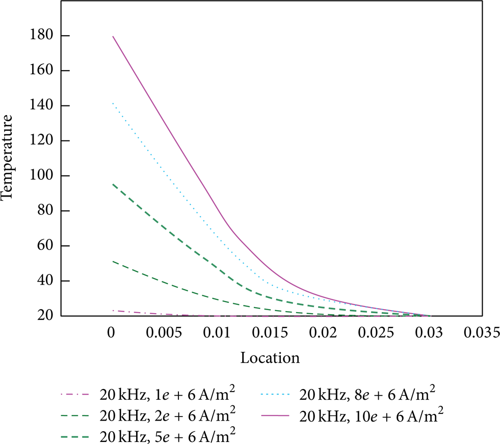
Figure 30 shows the temperature distribution along the x-axis direction on the upper surface under different eddy current densities with 4's heating time and 20 kHz operating frequency. The curves are corresponding to the eddy density of 10*10⁶ A/m², 8*10⁶ A/m², 5*10⁶ A/m², 2*10⁶ A/m², and 1*10⁶ A/m² from top to bottom. From the figure we can see that the greater the eddy current density is, the more dramatic the lateral variation temperature will be, which is similar to frequency influencing temperature. Therefore, in the design of the sensor, we can refer to the simulation results and choose rational argument.

Figure 30:

The temperature distribution along the x-axis under different vortex densities.

5.3. Heating Test Results

As the internal temperature of the plate cannot be measured, we can only test the upper surface point, lower surface point, and the upper surface point along the x-axis during the heating test. The temperature distribution can be generally understood. The test and simulation conditions are frequency 20 kHz, current density 5*10⁶ A/m², and the distance between coil and workpiece 6 mm. Temperature measurement instruments are the handheld infrared thermometer made by Fluke company.

The results are shown in Figure 31. It should be noted that the simulated temperature of the workpiece can be sharply increased in a short time, but temperature changes relatively slowly in practice. So the length of the simulation was 12's, and the duration of the test was 30's; otherwise it cannot explicit the trend of the actual temperature.

Figure 31:

The experiments and simulation data comparison.

The temperature of point A on the upper surface is measured every 1's; the curve was shown in Figure 31(a). Visibly, the trends of actual results and simulation results have a good agreement, but the temperature gently rises to 650 degrees and then becomes stable in practice. There was no local overheating phenomenon. According to the simulation, the maximum temperature is 1100 degrees and stable at around 850 degrees. The causes of deviation from the simulation aspect and the numerical simulation of the actual problem are idealized; it is impossible to completely describe the practical problems, such as the distribution of magnetic field lines, heat transfer, thermal radiation, and changes in material properties. From the test aspect, although the current density is the same as simulation, but there are reactive power and various losses, the power will not be completely absorbed by the workpiece. Therefore, the temperature rises relatively flat. In addition, the hand-wound heating coil also affects the power transmission and distribution of eddy currents due to its unevenness.

Similarly, to measure the temperature of point C every 1's, the curve was shown in Figure 31(b). The figure shows that the trends of the two are the same, but the temperature rise was still relatively slow. The temperature of C point was about 148 degrees when heated 30's. The reason of the deviation in addition to the limitations of the simulation itself, the heating time is anther. 30's is longer than the simulation time, so more heat transfers to the lower surface, and the final temperature is higher than the simulation result. In addition, the workpiece is isotropic and has edge effect, so that there are still some distributions of magnetic field lines along the lower surface and influence of temperature of the lower surface.

Figure 31(c) shows the comparison between simulation and experiment when heating is 10's. The data is recorded every 1 cm from the center along the x-axis, although the simulation results show that the temperature of the workpiece center is unchanged. The heat will transfer to the center in actual, combined with the distribution of magnetic lines in center position and eddy heat of itself, so it was nearly 200 degrees at the 10's. Further, the size of the workpiece is relatively small; good thermal conductivity of the sheet and the emission distribution of magnetic lines are very good. Therefore, the actual experiment does not have the result as simulation. The edge effect and end effects make the edge temperature of the workpiece rise rapidly, and the heat also transfers to the surrounding quickly, which also reduces the temperature difference. It should be noted that the data is measured by artificial way, where there will be some errors.

Based on the above results and analysis, the test results and simulation results are more consistent on the variation tendency, but the temperature rises relatively slowly in the test and lags the simulation results. The maximum temperature of the upper surface is lower than the simulation, and the final temperature of lower surface is higher than the simulation. In space, the lateral distribution of the temperature of the upper surface does not appear the temperature difference region as shown in the simulation. This may be caused by the numerical simulation to simulate that the real problem has some limitations; the experimental parameters, such as the power factor, affect the impact of the coil, the escape of magnetic field lines, and manual measurement.

5.4. Temperature Distribution Model

As a highly nonlinear system, there are many factors that affect the temperature distribution of the workpiece in single-sided electromagnetic induction heating, such as heating time t, the current frequency f, the current density J_s, and other attributes of materials [10]. In the simulation, the characteristics of the material are integrated into account and we give the simulation results under different conditions. Since the interaction between various fields in the heating process is very complex, it is impossible to use an accurate model to express the actual relationship between them. In order to explore the relationship between the surface temperature distribution characteristics and various parameters in single-sided heating process, we make use of a model to express the relationship between parameters based on experience and related graphics. The temperature distribution model is shown as follows:

T = a_{0} t^{2} + a_{1} t + a_{2} J_{S}^{2} + a_{3} J_{S} + a_{4} f^{2} + a_{5} f + a_{6} h^{3} + a_{7} h^{2} + a_{8} h + a_{9} X^{2} + a_{10} X + a_{11},

(21)

where t (s) is the heating time, J_S (*10⁶ A/m²) represents vortex density, f (kHz) is the operating frequency, h (mm) is the depth from the surface, and X (mm) is the distance to the center of the workpiece. This model can express both effects of the nonlinear parameters on the temperature distribution and simplify the process of identification by using linear relationship between each item.

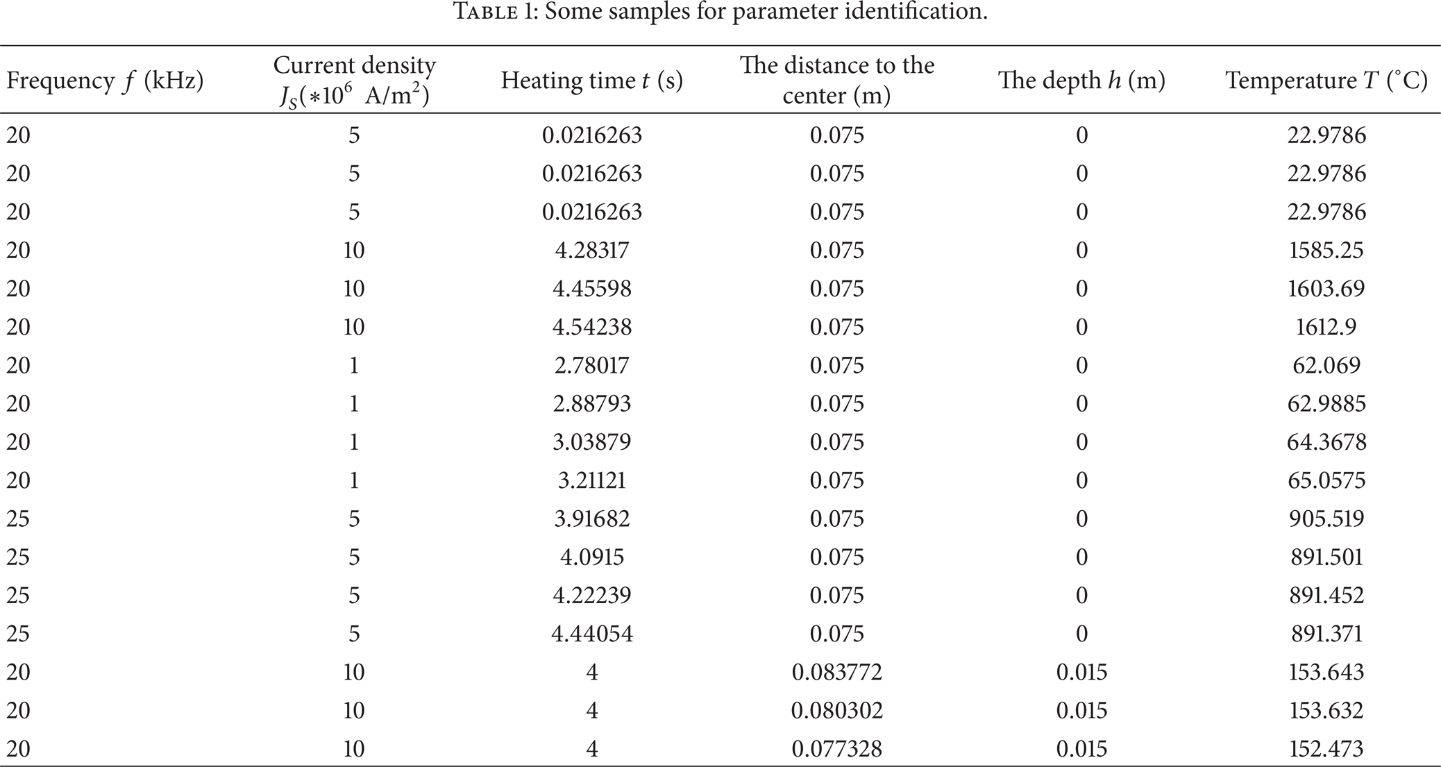
Since it is impossible to measure the temperature of the middle layer plate and get too many consecutive data, therefore, the simulation results are used for identification. We obtain the original data to be nearly 3000; part of the data is shown in Table 1.

Table 1:

Some samples for parameter identification.

Frequency f (kHz)	Current density J_S(*10⁶ A/m²)	Heating time t (s)	The distance to the center (m)	The depth h (m)	Temperature T (°C)

20	5	0.0216263	0.075	0	22.9786
20	5	0.0216263	0.075	0	22.9786
20	5	0.0216263	0.075	0	22.9786
20	10	4.28317	0.075	0	1585.25
20	10	4.45598	0.075	0	1603.69
20	10	4.54238	0.075	0	1612.9
20	1	2.78017	0.075	0	62.069
20	1	2.88793	0.075	0	62.9885
20	1	3.03879	0.075	0	64.3678
20	1	3.21121	0.075	0	65.0575
25	5	3.91682	0.075	0	905.519
25	5	4.0915	0.075	0	891.501
25	5	4.22239	0.075	0	891.452
25	5	4.44054	0.075	0	891.371
20	10	4	0.083772	0.015	153.643
20	10	4	0.080302	0.015	153.632
20	10	4	0.077328	0.015	152.473

Using the least squares method for model parameter identification [18] such as

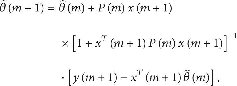
\hat{θ} (m + 1) = \hat{θ} (m) + P (m) x (m + 1) \times {[1 + x^{T} (m + 1) P (m) x (m + 1)]}^{- 1} \cdot [y (m + 1) - x^{T} (m + 1) \hat{θ} (m)],

(22)

1 + x^T(m + 1)P(m)x(m + 1) is a scalar, which simplifies the calculations by avoiding the matrix inversion.

Using the sample data to estimation parameter, we can obtain the coefficients of formula

T = 0.79 t^{2} - 0.48 t - 7.81 J_{S}^{2} + 172.4 J_{S} + 0.088 f^{2} - 3.63 f - 0.12 h^{3} + 6.57 h^{2} - 113.4 h - 0.042 X^{2} + 7.00 X - 140.2 .

(23)

The sample temperature curve and the temperature curve derived from the model are shown in Figure 32. The figure shows that the sample values and calculation results are achieve in good agreement on the trend for most data, but there are still some larger errors in some cases. Possible causes of errors are the following aspects: using some simple functions to replace the complex coupling relationship in modeling; the model ignores the material characteristics and the interaction between other parameters; only considering the static status.

Figure 32:

The contrast curve of sample and simulation.

6. Conclusions

This paper studies the single-sided induction heating. The primary heating circuit, control circuit, and auxiliary circuit are designed. The IGBT as the main power device is used to realize the system, and a single IGBT driver and protection circuit are designed. The heating test and theoretical analysis are very consistent, and the temperature trends of simulation and test performed are relatively consistent. We make use of the least squares theory to establish the preliminary mathematical model of the system. The following works will be needed: study the influence of the induction heating coil on heating effect and the magnetic field distribution in order to design the efficient heating coil for single-sided occasion; study the principle of electromagnetic induction heating further to explore a more realistic mathematical model to describe the heating system and provide a strong theoretical guidance for the system design.

Conflict of Interests

The authors declarethat there is no conflict of interests regarding the publication of this paper.

References

Liu

Chen

Lin

, and Liu

, “Thermo-mechanical analysis of a wafer level packaging by induction heating,” in Proceedings of the International Conference on Electronic Packaging Technology and High Density Packaging, pp. 1–5, July 2008.

Alwash

J. H. H.

and Sultan

S. K.

, “Performance prediction of single-sided induction heating system,” IEEE Transactions on Energy Conversion, vol. 25, no. 4, pp. 1057–1062, 2010.

Chen

S.-C.

Jong

W.-R.

, and Chang

J.-A.

, “Dynamic mold surface temperature control using induction heating and its effects on the surface appearance of weld line,” Journal of Applied Polymer Science, vol. 101, no. 2, pp. 1174–1180, 2006.

Tavakoli

M. H.

Karbaschi

, and Samavat

, “Influence of workpiece height on the induction heating process,” Mathematical and Computer Modelling, vol. 54, no. 1–2, pp. 50–58, 2011.

Josifović

Popović-Gerber

, and Ferreira

J. A.

, “New double sided SMT power inductor,” in Proceedings of the International Power Electronics Conference (IPEC '10), pp. 3144–3150, June 2010.

Nerg

and Partanen

, “A simplified FEM based calculation model for 3-D induction heating problems using surface impedance formulations,” IEEE Transactions on Magnetics, vol. 37, no. 5, pp. 3719–3722, 2001.

Zhong

, and Sheng

, “Effects of PRC supply load-variance upon inverter switch states,” Journal of Xi'an University of Technology, vol. 18, no. 1, pp. 31–34, 2002.

Jun-sheng

, “Analysis of load electrical characteristics for induction heating systems of high frequency,” Industrial Heating, vol. 37, no. 2, pp. 56–58, 2008.

Theron

P. C.

and Ferreira

J. A.

, “Zero voltage switching partial series resonant converter,” IEEE Transactions on Industry Applications, vol. 31, no. 4, pp. 879–886, 1995.

10.

Zhou

, Research on current-fed parallel resonant high-frequency inducton heating power supply [M.S. thesis], Zhejiang University, Hangzhou, China, 2005.

11.

Zhang

Song

Zhou

Guo

, and Miao

, “A novel half-bridge series-resonant high-frequency induction welding power supply,” Acta Scientiarum Naturalium Universi-tatis Nankaiensis, vol. 42, no. 2, pp. 77–81, 2009.

12.

Jain

P. K.

and Dewan

S. B.

, “A performance comparison of full- and half-bridge series resonant inverters in high-frequency high-power applications,” IEEE Transactions on Industry Applications, vol. 26, no. 2, pp. 317–323, 1990.

13.

Candeo

Ducassy

Bocher

, and Dughiero

, “Multi-physics modeling of induction hardening of ring gears for the aerospace industry,” IEEE Transactions on Magnetics, vol. 47, no. 5, pp. 918–921, 2011.

14.

Gong

Hagel

Zhang

, and Unbehauen

, “On the 3-D eddy current field coupled to the heat transfer of induction heating of a slab,” in Proceedings of the 30th IEEE Industry Applications IAS Annual Meeting, pp. 1952–1956, October 1995.

15.

Rotti

Acharya

Bandyopadhyay

, “Analysis of residual ion dump (RID) of diagnostic neutral beam (DNB) injector for ITER,” in Proceedings of the 23rd IEEE/NPSS Symposium on Fusion Engineering (SOFE '09), pp. 1–4, June 2009.

16.

Sadeghipour

Dopkin

J. A.

, and Li

, “A computer aided finite element/experimental analysis of induction heating process of steel,” Computers in Industry, vol. 28, no. 3, pp. 195–205, 1996.

17.

Mahmoudi

Rahim

N. A.

, and Hew

W. P.

, “Axial-flux permanent-magnet machine modeling, design, simulation and analysis,” Scientific Research and Essays, vol. 6, no. 12, pp. 2525–2549, 2011.

18.

Wang

, “Windowed least square algorithm based pmsm parameters estimation,” Mathematical Problems in Engineering, vol. 2013, Article ID 131268, 11 pages, 2013.

Single-Sided Electromagnetic Induction Heating Based on IGBT

Abstract

1. Introduction

2. The Principle of Single Induction Heating

3. Design of a Half-Bridge Series Resonance Circuit

4. The Design of the Induction Heating System

4.1. The Topology of the System

4.2. The Selection of Operating Frequency and Power

4.3. IGBT Drive

4.4. The Resonant Circuit Design

4.4.1. Induction Coil Design

4.4.2. Matching Transformer Design

4.4.3. Determine the Value of Resonant Inductance of the Inductor

4.5. Safeguard

4.5.1. The Buffer Circuit Design of IGBT

4.5.2. Current Detection and Protection Circuit

4.5.3. Temperature Detection and Protection Circuit

5. Simulation Results

5.1. Main Circuit Simulation

5.2. The Temperature and Electromagnetic Field Simulation in ANSYS

5.2.1. The System Analysis under Given Conditions

5.2.2. The Temperature Distribution under Different Frequencies

5.2.3. The Effect of Eddy Current Density on the Temperature Distribution

5.3. Heating Test Results

5.4. Temperature Distribution Model

6. Conclusions

Conflict of Interests

References