Multivariate Storage Degradation Modeling Based on Copula Function

Abstract

A generalized statistical model is introduced in the paper to qualify the reliability of a dormant system which has multiple de-pendent performance characteristics (PCs). In the model, the univariate degradation process of each PC is governed by Wiener processes with time transformation, and multivariate copula function is used to describe the dependence among the PCs. The parameters of Wiener process and copula function in the model are supposed to depend on temperature and their relationship can be expressed by the transformation functions. Based on the CSADT data, the parameters in the model can be calculated by the maximum likelihood estimate. Then the transformation functions can be derived from these estimated values by the regression analysis. Particularly, as the storage temperature is not constant, the variation of the temperature is taken into consideration in the model. In the end, as an illustration for the given model, a case application is presented as an example.

1. Introduction

Engineering storage degradation tests allow industry to assess the storage reliability of high reliable products that do not fail easily under accelerated stress. However, though there is a lot of literature [1–5] on the estimation of system reliability based on the multivariate or bivariate degradation data, most of them are typically based on two assumptions. First, the degraded PCs are independent or following a certain kind of multivariate distribution. Second, the stress exerted on the product is constant. But in practice, these assumptions may not be realized. If we want to qualify the storage reliability of a dormant system with multiple degraded PCs more accurately, the relationship between these degraded PCs and the variation of the stress should be taken into account.

A generalized case is assumed that a dormant system has multiple degraded PCs and each PC leads to a failure mechanism of the system. But the relationship between these PCs is unknown, which means that the PCs may not be independent. Then how to acquire system's dependent reliability is the problem we have to solve.

This paper considers temperature as the only stress in the storage environment, and a statistical model is introduced to qualify the reliability of a dormant system based on the dependent CSADT data. In the model, the univariate degradation process of each PC is governed by Wiener processes with time transformation, and the relationship between the PCs is described by multivariate copula function. It is also proposed that each parameter of Wiener processes and copula function can be expressed by a function of stress, which is denoted as transformation function. All these parameters mentioned above can be estimated by MLE. Based on these estimated values, the transformation functions are directly derived by the regression analysis. Particularly, a variable-stress storage life modeling method is introduced to describe the variation of the stress. At the end of this paper, as an illustration for the given model, a case application is presented as an example.

The rest of the paper is organized as follows. In Section 2, a multivariate degradation model is introduced. In Section 3, an inference method is given to get the parameters required. Based on the real storage environment, a storage life modeling method is presented in Section 4. In Section 5, a case application is given to illustrate the proposed model. Finally, some conclusions are made in Section 6.

2. Multivariate Degradation Model

2.1. Assumptions

It is assumed that the dormant system and the accelerated degradation storage tests in this research fulfill the following assumptions.

1. The system has multiple degraded PCs and each PC leads to a failure mechanism of the system. These degraded PCs may not be independent.

2. No catastrophic failures occur during the storage period.

3. The process of the degradation only depends on temperature, which is the only stress considered in this model.

2.2. Univariate Degradation Model

The univariate degradation process is modeled by a Wiener process, which can be defined as:

$W=\eta \tau \left(t\right)+\sigma B\left(\tau \left(t\right)\right),$

(1)

where B(·) is the standard Wiener process and η is the drift parameter. σ is the diffusion parameter. τ(t) is the time transformation function. Basic properties of a Wiener process may be found in the work of Cox and Miller [6].

The transformation function τ(t) largely depends on the mechanism of degradation in the given application. The most widely used transformation functions are the following two forms:

$\tau \left(t\right)=1-\exp (-\lambda t^{\gamma })$

(2)

$\tau \left(t\right)=t^{\lambda },$

(3)

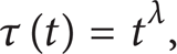
where λ and γ are transformation parameters.

The exponential time transformation in (2) is suitable for many applications in which the degradation approaches a saturation point where deterioration ends. One of the typical cases is the oxidation [7, 8]. The power time transformation in (3) is used in the case where the degradation continues to increase without being bound. This kind of transformation is more generalized and is used in many cases like the degradation of lead [9], coating corrosion of steel [10], and so on.

If a multivariate degraded system has n degraded PCs, for the ith degraded PC, it is assumed that the relationship between the transformed stress and the transformed parameters is linear as follows:

$\begin{array}{c}{B}_i\left({\sigma }_i\right)=b_{i\mathrm{0}}+b_{i\mathrm{1}}H\left(s_i\right)\\ C_i\left({\lambda }_i\right)=c_{i\mathrm{0}}+c_{i\mathrm{1}}H\left(s_i\right),\end{array}$

(4)

where s_i is the stress, and B _i (σ _i ), C _i (λ _i ), and H _i (s _i ) are the transformation functions. In this research, the transformation types of these four transformation functions are supposed to be nonparametric transformations, which were proved to be very sufficient in many studies [11]. The typical nonparametric transformations are logarithmic transformation, exponential transformation, reciprocal transformation, and so on.

As to the drift parameter η, its transformation function is

${\mu }_i=\exp \left(a+\frac{b}{s}\right).$

(5)

This transformation function is the Arrhenius function which is widely used in the reliability field.

2.3. The Multivariate Degradation Model

According to the independent increment property of the Wiener process, for the ith PC's degradation process, the marginal distribution function at the moment of t is as follows:

$W^{\left(i\right)}\left(\tau \left(t\right)\right)~N\left({\eta }_i\tau \left(t\right),{\sigma }_i^{\mathrm{2}}\tau \left(t\right)\right).$

(6)

Suppose the system has n degraded PCs, then we can get the function of system reliability at the moment of t:

$R\left(t\right)=P\left\{W^{\left(\mathrm{1}\right)}\left(\tau \left(t\right)\right)<l_{\mathrm{1}},W^{\left(\mathrm{2}\right)}\left(\tau \left(t\right)\right)<l_{\mathrm{2}},\dots ,W^{\left(n\right)}\left(\tau \left(t\right)\right)<l_n\right\}=P\left\{W^{\left(\mathrm{1}\right)}<l_{\mathrm{1}}\mid t,W^{\left(\mathrm{2}\right)}<l_{\mathrm{2}}\mid t,\dots ,W^{\left(n\right)}<l_n\mid t\right\},$

(7)

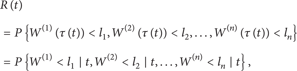
where l_i is the threshold value of the ith PC's degradation process. $P(W^{(i)}<l_i\mid t)$ is the probability of $W^{(i)}<l_i$ at the moment of t.

According to Sklar's Theorem [12], (7) can be expressed as follows, which was first introduced by Sari [13]:

$R\left(t\right)=P\left\{W^{\left(\mathrm{1}\right)}<l_1\mid t,W^{\left(\mathrm{2}\right)}<l_{\mathrm{2}}\mid t,\dots ,W^{\left(n\right)}<l_n\mid t\right\}=H(l_{\mathrm{1}},l_{\mathrm{2}},\dots ,l_n\mid t)=C\left(G^{\left(\mathrm{1}\right)}\left(l_{\mathrm{1}}\mid t\right),G^{\left(\mathrm{2}\right)}\left(l_{\mathrm{2}}\mid t\right),\dots ,G^{\left(n\right)}\left(l_n\mid t\right)\right),$

(8)

where $G^{(i)}(w\mid t)$ is the marginal distribution function of degradation process W⁽ⁱ⁾ at the moment of t.

From property of Wiener process [6], we can get the CDF of the marginal distribution function $G^{(i)}(w\mid t)$ as follows:

$G^{\left(i\right)}\left(wt\right)=\Phi \left(\frac{w-{\eta }_i\tau \left(t\right)}{{\sigma }_i\sqrt{\tau \left(t\right)}}\right).$

(9)

In this paper, we choose the Frank copula [13] as the copula function in (8), which is:

$C\left(\mathbf{u}\right)=-\frac{\mathrm{1}}{\theta }\ln [\mathrm{1}+\frac{\left(e^{-\theta u_{\mathrm{1}}}-\mathrm{1}\right)\left(e^{-\theta u_{\mathrm{2}}}-\mathrm{1}\right)\cdots (e^{-\theta u_d}-\mathrm{1})}{{\left(e^{-\theta }-\mathrm{1}\right)}^{d-\mathrm{1}}}],$

(10)

where $\mathbf{u}=\mathbf{(}{u}_1\mathbf{,}\dots ,u_d\mathbf{)}$ . Its generator function is

$\phi \left(t\right)=-\ln \left(\frac{e^{-\theta t}-\mathrm{1}}{e^{-\theta }-\mathrm{1}}\right),\hspace{1em}\theta \in \left(-\infty ,\infty \right).$

(11)

3. Inference Method

3.1. Parameters of Univariate Degradation Model

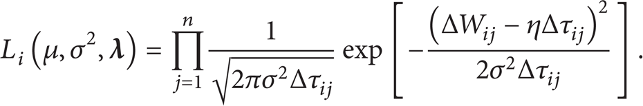
At first, we use MLE to estimate the parameters of Wiener process. Consider the case that m samples were put into test. Let us focus on the n + 1 observations (W _ij ,t _ij ) for the ith sample where j = 0, 1,…, n. Define ΔW _ij = W _ij -W_ij–1 and Δτ _ij = τ(t _ij )-τ(t_ij–1) where j = 1, 2,…, n, then we can get the likelihood function for the ith sample:

$L_i(\mu ,{\sigma }^{\mathrm{2}},\mathbf{\lambda })={\displaystyle \prod }_{j=\mathrm{1}}^n\frac{\mathrm{1}}{\sqrt{\mathrm{2}\pi {\sigma }^{\mathrm{2}}\Delta {\tau }_{ij}}}\exp \left[-\frac{{\left(\Delta W_{ij}-\eta \Delta {\tau }_{ij}\right)}^{\mathrm{2}}}{\mathrm{2}{\sigma }^{\mathrm{2}}\Delta {\tau }_{ij}}\right].$

(12)

Suppose the transformation parameter λ in function τ(t) is fixed, then we can get the maximum likelihood estimators of η, σ² by maximizing (12):

$\begin{array}{c}{\widehat{\eta }}_i\left(\lambda \right)=\frac{W_{ij}-W_{i\mathrm{0}}}{{\tau }_{ij}-{\tau }_{i\mathrm{0}}}\\ {\widehat{\sigma }}_i^{\mathrm{2}}\left(\lambda \right)=\frac{\mathrm{1}}{n}{\displaystyle \sum }_{j=\mathrm{1}}^n\frac{{\left[\Delta W_{ij}-{\widehat{\eta }}_i\left(\lambda \right)\Delta {\tau }_{ij}\right]}^{\mathrm{2}}}{\Delta {\tau }_{ij}}.\end{array}$

(13)

Substitute these estimators to (10), the likelihood function can be modified as:

$L_i\left(\mathbf{\lambda }\right)={\left[\mathrm{2}\pi {\widehat{\sigma }}^{\mathrm{2}}\left(\mathbf{\lambda }\right)\right]}^{-n/\mathrm{2}}\exp (-\frac{n}{\mathrm{2}}){\displaystyle \prod }_{j=\mathrm{1}}^n{\left(\Delta {\tau }_{ij}\right)}^{-\mathrm{1}/\mathrm{2}}.$

(14)

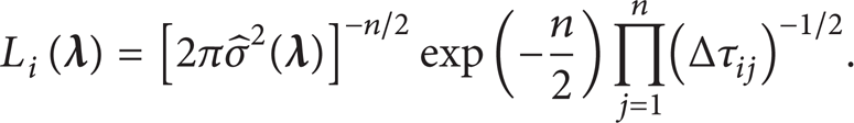
This is a function of λ, so the maximum likelihood estimator $\widehat{\lambda }$ can be calculated by maximizing (14). If $\widehat{\lambda }$ is gotten, $\widehat{\eta }$ and $\widehat{\sigma }$ can be directly derived from (13).

3.2. Kendall's Tau

Kendall's tau is one of the most commonly used measures of association. In this paper, we use 2-dimensional τ₂ to measure the dependence of the multivariate degraded PCs.

Let us consider a system including two degraded PCs, which is denoted as X and Y. Let (X₁,Y₁) and (X₂,Y₂) be an independent pair of observations. Then Kendall's tau of X and Y can be defined as the probability of concordance minus the probability of discordance which can be written as follows:

${\tau }_{\mathrm{2}}(X,Y)=P[(X_{\mathrm{1}}-X_{\mathrm{2}})(Y_{\mathrm{1}}-Y_{\mathrm{2}})>\mathrm{0}]-P\left[\left(X_{\mathrm{1}}-X_{\mathrm{2}}\right)\left(Y_{\mathrm{1}}-Y_{\mathrm{2}}\right)<\mathrm{0}\right].$

(15)

The definition of concordance and discordance is first introduced by Kruskal [14] and Lehmann [15].

Here (15) is

${\tau }_{\mathrm{2}}\left(X,Y\right)=P[(X_{\mathrm{1}}-X_{\mathrm{2}})(Y_{\mathrm{1}}-Y_{\mathrm{2}})>\mathrm{0}\mid t]-P\left[\left(X_{\mathrm{1}}-X_{\mathrm{2}}\right)\left(Y_{\mathrm{1}}-Y_{\mathrm{2}}\right)<\mathrm{0}\mid t\right].$

(16)

This means the difference between concordance and discordance of PCs’ observation data at certain measurement time.

Then let us consider d-dimension τ _d , suppose X₁,X₂,…, X _d are continuous random variables, and can be expressed by the d-dimension vector X = (X₁,X₂,…, X _d ). From the paper of Genest et al. [16], the d-dimension τ _d (X) can be expressed as follows:

${\tau }_d\left(\mathit{X}\right)=\frac{{\mathrm{2}}^{d-\mathrm{1}}}{{\mathrm{2}}^{d-\mathrm{1}}-\mathrm{1}}{\displaystyle \sum }_{\begin{array}{c}A\subset D\\ \mathrm{1}<\left|A\right|<d\end{array}}{\left(-\frac{\mathrm{1}}{\mathrm{2}}\right)}^{\left|A\right|}\left({\mathrm{2}}^{\left|A\right|-\mathrm{1}}-\mathrm{1}\right){\tau }_{\left|A\right|}\left({\mathit{X}}_A\right),$

(17)

where A⊂D = {1,…, d}, $\left|A\right|$ is the length of set A. X A is the subvector of X and its dimension is $\left|A\right|$ . The components of X A are X _i for all i∈A.

Thus d-dimension τ _d (X) can be expressed by τ₂(X _i ,X _j ), where i,j∈{1,…, d} and i≠j.

Like (4), the τ _d is supposed to have a liner relationship with the transformed stress, which can be expressed as follows:

$D\left({\tau }_d\right)=d_{i\mathrm{0}}+d_{i\mathrm{1}}H\left(s_i\right).$

(18)

3.3. The Relationship between Kendall's τ and Frank Copula Function

Let ψ(t) = φ⁻¹(t), we can get the relationship between τ _d and generate function φ(t) of Frank copula in (10), which is introduced by Genest et al. [16]:

$\begin{array}{c}{\tau }_d=\frac{\mathrm{1}}{{\mathrm{2}}^{d-\mathrm{1}}-\mathrm{1}}\left[-\mathrm{1}+{\mathrm{2}}^{d}E\left\{\psi \left(R\right)\right\}\right],\\ E\left\{\psi \left(R\right)\right\}=\frac{{\left(-1\right)}^d}{\left(d-1\right)!{\int }_0^{{\psi }^{-1}\left(0\right)}{r}^{d-1}\psi \left(r\right){\psi }^{\left(d\right)}\left(r\right)dr},\end{array}$

(19)

where ${\psi }^{(d)}(r)$ denotes the dth derivative of ψ(r).

Note φ(t) is the function of copula parameter θ. Thus if we can get τ _d from the d-dimension degradation system, then θ can be derived from (19).

4. The Storage Life Modeling under the Real Storage Environment

4.1. Basic Assumptions on the Storage Temperature

In the real storage environment, the temperature could not be considered as a constant. In fact, from Figure 1, we can conclude that the difference in daily average temperature exceeds 20°C in a year. But for most of the days, the variation of the temperature in a day is controlled to be within 3°C. Given the fact above, we can approximately consider the storage temperature following these two assumptions.

Figure 1:

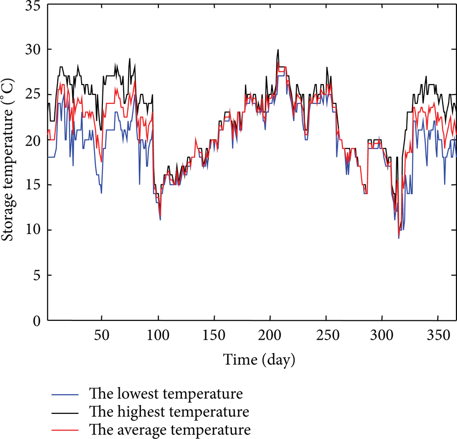
The annual storage temperature data.

(1) The storage temperature is approximately constant during a day.

(2) The daily average temperature varies in a wide range in a year, and this kind of variation must be taken into consideration.

4.2. The Storage Life Modeling Method

From the assumptions above, the degradation process can be expressed in Figure 2, in which S _i represents the ith stress and τ represents the transformed time τ(t).

Figure 2:

The degradation process under storage environment.

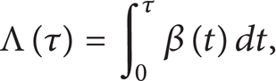
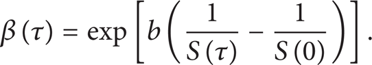
First, let ${\alpha }_i={\mu }_i/{\mu }_{i-\mathrm{1}}$ , from (5), we can derive that:

${\alpha }_i=\frac{{\mu }_i}{{\mu }_{i-\mathrm{1}}}=\exp \left[b\left(\frac{\mathrm{1}}{s_i}-\frac{\mathrm{1}}{s_{i-\mathrm{1}}}\right)\right].$

(20)

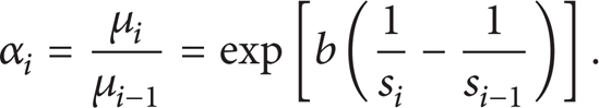
Let α₀ = 1 and let ${\beta }_i={\prod }_{r=0}^i{\alpha }_r$ , then:

${\beta }_i=\exp \left[b\left(\frac{\mathrm{1}}{s_i}-\frac{\mathrm{1}}{s_{\mathrm{0}}}\right)\right].$

(21)

From variable-stress degradation model introduced by Doksum and Hoyland [17], we can get the following conclusion.

Let

$\mathrm{\Lambda }\left(\tau \right)={\displaystyle \sum }_{r=\mathrm{0}}^{i-\mathrm{1}}{\beta }_r\left({\tau }_{r+\mathrm{1}}-{\tau }_r\right)+{\beta }_i\left(\tau -{\tau }_i\right),$

(22)

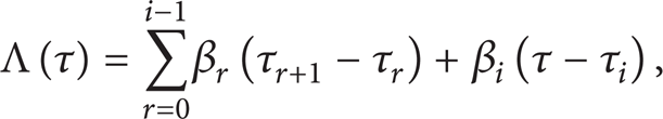
where τ _i ≤ τ ≤ τ_{i + 1}, i = 1,…, n, then the degradation path at time t can be expressed as follows:

$W\left(\tau \right)=W_{\mathrm{0}}\left(\mathrm{\Lambda }\left(\tau \right)\right),$

(23)

where W₀(·) means that the degradation path is under the initial stress S0.

From (9), we can get the distribution function of W₀(Λ(τ)):

$G_{\mathrm{0}}\left(w_{\mathrm{0}}\mid \tau \right)=\Phi \left(\frac{w_{\mathrm{0}}-{\mu }_{\mathrm{0}}\mathrm{\Lambda }\left(\tau \right)}{{\sigma }_{\mathrm{0}}\sqrt{\mathrm{\Lambda }\left(\tau \right)}}\right),$

(24)

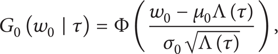
where η₀ and σ₀ are the drift parameter and diffusion parameter under stress S0.

If i→∞, then t_{r + 1}-t _r →0, r∈[0,i]. β _i can be denoted as continuous function β(τ).

Consider the following:

$\mathrm{\Lambda }\left(\tau \right)={{\displaystyle \int }}_{\mathrm{0}}^{\tau }\beta \left(t\right)dt,$

(25)

where

$\beta \left(\tau \right)=\exp \left[b\left(\frac{\mathrm{1}}{S\left(\tau \right)}-\frac{\mathrm{1}}{S\left(\mathrm{0}\right)}\right)\right].$

(26)

According to the assumptions made in Section 4.1, (22) can be modified as follows:

$\mathrm{\Lambda }\left(\tau \right)=e^{-b/S\left(\mathrm{0}\right)}{{\displaystyle \int }}_{\mathrm{0}}^{\tau }\exp \left(\frac{b}{S\left(t\right)}\right)dt=e^{-b/S_{\mathrm{0}}}{\displaystyle \sum }_{i=\mathrm{0}}^{t-\mathrm{1}}\left[\tau \left(i+\mathrm{1}\right)-\tau \left(i\right)\right]\exp \left(\frac{b}{S_i}\right).$

(27)

Let R _l denote system's threshold value of reliability; we can give system's storage life modeling method.

Step 1. Get the initial stress S0, and use (4) and (5) to get the wiener parameters of each degradation process under S0, respectively. Finally set n = 1.

Step 2. Fetch the nth day's storage temperature S _n , and use (17), (18), and (19) to calculate the copula parameter θ. Then nth day's reliability R _n can be derived.

Step 3. If R _n >R _l , then n = n + 1, go to the Step 1. Otherwise we can get degradation system's storage life T _s = n.

Specifically, since we only have storage temperature data in one year, it is impossible for us to get daily temperature's distribution function.

Given the fact that the storage temperature is changed with the seasons, we can assume every year's annual temperature data are approximately the same. Only in this way we can get the storage temperature data.

5. Case Application

5.1. Background

The purpose of the program is to qualify the reliability of a kind of dormant system which includes two weak units, DRO, and LNB-DRO. Both DRO and LNB-DRO can only work properly under a certain range of operating frequency. However, the real ranges of frequency of them increase with time even in the storage environment. Therefore, for either DRO or LNB-DRO, if the increment of the frequency goes over the threshold value, the whole dormant system would fail. The threshold values of DRO and LNB-DRO are already known to be 0.2 MHz and 0.1 MHz, respectively.

In order to get the degradation data, accelerated storage degradation test was carried out. The test items are certain types of DRO and LNB-DRO. Ten test samples were put into test in each temperature level for both DRO and LNB-DRO, respectively. Three test temperature levels, 50°C, 60°C, and 70°C, were applied for the two kinds of samples. Finally, 26 readings were recorded for each of the samples.

As for the transformation function, given that there are no clear saturated boundaries in the degradation processes of DRO and LNB-DRO, it is convenient to choose the power time transformation as the time transformation function so τ(t) = t^λ in (1).

5.2. Estimation of DRO's Degradation Parameters

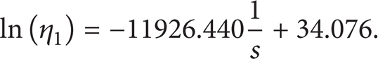
In the following, we are going to estimate the parameters of DRO's degradation process. Denote i = 1 in (6), then λ₁, η₁, and σ₁² are the parameters that should be estimated. Using the inference method in Section 3, we can get the estimate of λ₁, which is denoted as ${\widehat{\lambda }}_1$ . Then from (13), and (14), ${\widehat{\eta }}_1$ , ${\widehat{\sigma }}_1^2$ , and ${\widehat{\lambda }}_{\mathrm{1}}$ can be calculated.

These three parameters are estimated for each of 10 samples on the three temperature levels, respectively. Try to plot these estimates against each kind of nonparametric transformations of the absolute temperature mentioned in Section 2.2. We can get the transformation function for each of the parameters.

Plot $\ln {\widehat{\eta }}_1$ against 1/s in Figure 3, we can prove that (5) is right. From the regression analysis, we can get the transformation function of ${\widehat{\eta }}_1$ :

$\ln \left({\eta }_{\mathrm{1}}\right)=-\mathrm{11926.440}\frac{\mathrm{1}}{s}+\mathrm{34.076}.$

(28)

Figure 3:

Plot of $\ln {\widehat{\eta }}_{\mathrm{1}}$ against 1/s.

As to the ${\widehat{\sigma }}_1^2$ , B₁(σ₁), and H(s) in (4) is ln⁡(η₁) and 1/s, respectively. Plot $\ln {\widehat{\sigma }}_1^2$ against 1/s in Figure 4.

Figure 4:

Plot of $\ln {\widehat{\sigma }}_1^2$ against 1/s.

Given that the relationship between them is linear, the transformation function can be directly calculated as follows:

$\ln \left({\widehat{\sigma }}_1^2\right)=-\mathrm{13890.171}\frac{\mathrm{1}}{\text{s}}+\mathrm{38.515}.$

(29)

At last, plot ${\widehat{\lambda }}_{\mathrm{1}}$ against 1/s in Figure 5.

Figure 5:

Plot of ${\widehat{\lambda }}_1$ against 1/s.

From Figure 4 we can notify that λ₁ is approximately independent of 1/s. Then λ₁ can be considered as a constant. Its value can be calculated as follows:

${\lambda }_{\mathrm{1}}=\mathrm{0.524}.$

(30)

5.3. Estimation of LIN-DRO's Degradation Parameters

The procedures of estimation of LIN-DRO's degradation parameters ${\widehat{\lambda }}_{\mathrm{2}}$ , ${\widehat{\eta }}_{\mathrm{2}}$ , and ${\widehat{\sigma }}_{\mathrm{2}}^{\mathrm{2}}$ are absolutely the same as what we have done in Section 5.2. Each set of transformed parameters was plotted against 1/s in Figures 6, 7, and 8.

Figure 6:

Plot of $\ln {\widehat{\eta }}_{\mathrm{2}}$ against 1/s.

Figure 7:

Plot of $\ln {\widehat{\sigma }}_2^2$ against 1/s.

Figure 8:

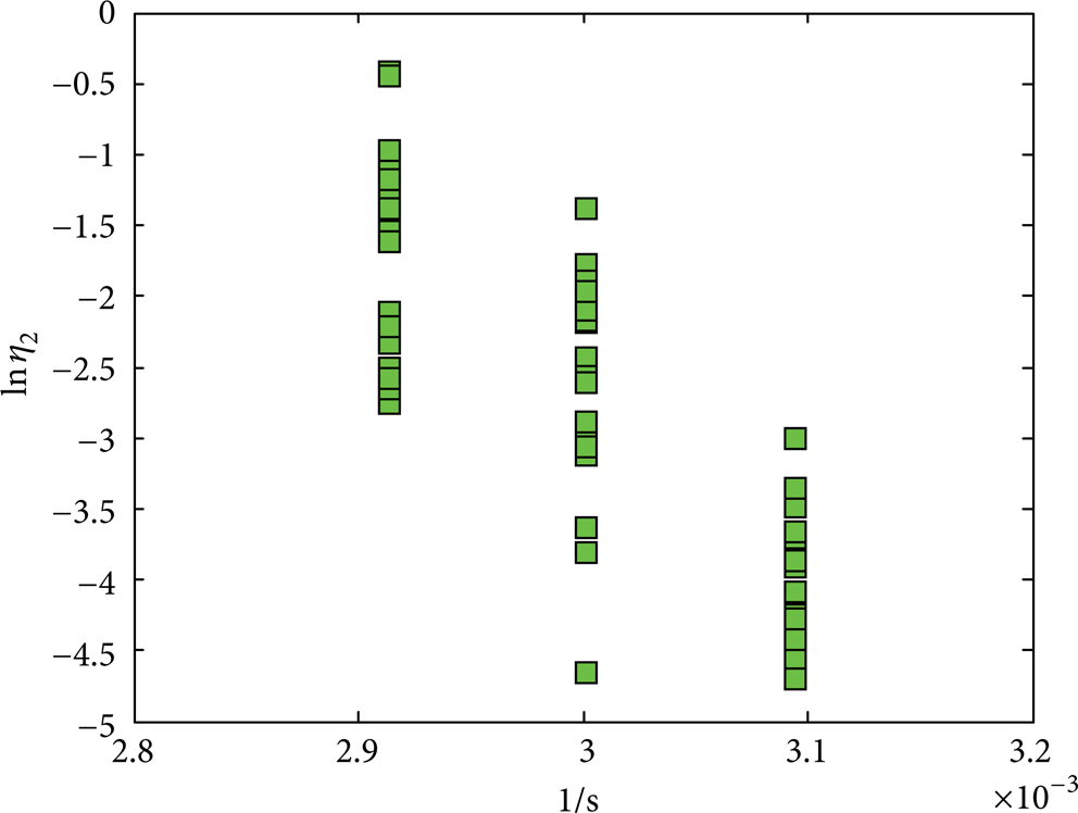
Plot of λ₂ against 1/s.

Based on these three plots, we can get the transformation functions of η₂, σ₂²:

$\begin{array}{c}\ln \left({\eta }_{\mathrm{2}}\right)=-\mathrm{15721.523}\frac{\mathrm{1}}{\text{s}}+\mathrm{44.688}\\ \ln \left({\sigma }_{\mathrm{2}}^{\mathrm{2}}\right)=-\mathrm{18368.363}\frac{\mathrm{1}}{\text{s}}+\mathrm{50.222}.\end{array}$

(31)

λ₂ is a constant, and its value is

${\lambda }_{\mathrm{2}}=\mathrm{0.678}.$

(32)

5.4. Estimation of Copula Parameters

Here we use kendall's tau to calculate the parameter of Frank copula. From (16), at each temperature level, we can get a set of ${\widehat{\tau }}_2$ between any two degraded processes from the two kinds of samples, respectively. Plot ${\widehat{\tau }}_2$ against 1/s in Figure 9.

Figure 9:

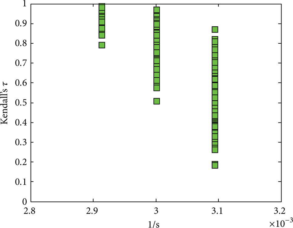
Plot of ${\widehat{\tau }}_2$ against 1/s.

From Figure 8, we can notify that D(τ₂) = τ₂ in (18). Using regression analysis, we can get the transformation function of τ₂:

${\tau }_{\mathrm{2}}=-\mathrm{1878.418}\frac{\mathrm{1}}{s}+\mathrm{6.394}.$

(33)

Since d = 2 in (10). From (19), we can get relationship between the Frank copula parameter θ and τ₂:

${\tau }_{\mathrm{2}}=\mathrm{1}+\mathrm{4}\frac{D_{\mathrm{1}}\left(\theta \right)-\mathrm{1}}{\theta },$

(34)

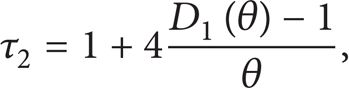
where $D_{\mathrm{1}}(\theta )=(\mathrm{1}/\theta ){\int }_{\mathrm{0}}^{\theta }(t/(e^t-\mathrm{1}))$ .

Then Frank copula parameter θ can be calculated.

5.5. Storage Life of the Multivariate Degradation System

Suppose the system's threshold value R _l = 0.4, from the storage life modeling method introduced in Section 4.2, we can give the algorithm of the storage life modeling method for this storage system.

Step 1. Use (28)–(31) to get the values of DRO's parameters η₁ and σ₁² and LNB-DRO's parameters η₂ and σ₂² under the initial stress S0. Then set n = 1.

Step 2. Get the nth day's temperature S _n from the storage temperature data, than the copula parameter θ can be derived from (33)–(34).

Step 3. From (10), (24), and (27) we can get the nth day's system reliability R _n , if R _n >R _l , then set n = n + 1, otherwise system’ s storage life can be derived, and the storage life T _s = n.

From the algorithm above, we can use matlab to get the storage life of the storage system, which is 5942 days.

6. Conclusions

This paper presents a statistical model to qualify the dependent reliability for a dormant system. We can conclude the following.

1. The time transformed Wiener process could be applied to model the univariate degradation process of each PC.

2. Kendall's tau and the parameters of Wiener process are supposed to depend on temperature and can be derived from the transformation functions.

3. Multivariate copula function is used to calculate the dependent reliability of the dormant system. In the case application, Frank copula function is chosen to be used in the real practice.

4. Based on the characteristics of storage temperature, the variation of the stress is taken into consideration in the life modeling method.

Conflict of Interests

The authors declare that there is no conflict of interests regarding the publication of this paper.